How Important Are Sectoral Shocks?
Enghin Atalay
June 16, 2014
Abstract
I quantify the contribution of sectoral shocks to business cycle ‡uctuations in ag-gregate output. I develop a multi-industry general equilibrium model in which each industry employs the material and capital goods produced by other sectors, and then estimate this model using data on U.S. industries’ sales, output prices, and input choices. Maximum likelihood estimates indicate that industry-speci…c shocks account for nearly two-thirds of the volatility of aggregate output, substantially larger than pre-viously assessed. Identi…cation of the relative importance of industry-speci…c shocks comes primarily from data on industries’intermediate input purchases, data that ear-lier estimations of multi-industry models have ignored.
1
Introduction
What are the origins of business cycle ‡uctuations? Do idiosyncratic micro shocks— disturbances at individual …rms or industries— have an important role in explaining short-run macroeconomic ‡uctuations? Or are shocks that prevail on all industries the predominant source?
I address these questions by constructing and estimating a multi-industry dynamic general equilibrium model in which both aggregate and industry-speci…c shocks have the potential to contribute to aggregate output volatility. I …nd that sectoral shocks are impor-tant: They account for more than three-…fths of the variation in aggregate output growth.
I thank Frank Limehouse and Arnie Reznek, for help with the data disclosure process. In addition, I am indebted to Fernando Alvarez, Thomas Chaney, Thorsten Drautzburg, Xavier Gabaix, Ali Hortaçsu, Oleg Itskhoki, Tim Kautz, Gita Khun Jush, Sam Kortum, Bob Lucas, Ezra Ober…eld, Nancy Stokey, Chad Syverson, Daniel Tannenbaum, and Harald Uhlig, for their helpful comments on earlier drafts, and to Erin Robertson, for her excellent editorial assistance. Disclaimer: Any opinions and conclusions expressed herein are those of the author and do not necessarily represent the views of the U.S. Census Bureau. All results have been reviewed to ensure that no con…dential information is disclosed. Updated versions of the paper can be found at home.uchicago.edu/~atalay/sectoral_shocks.pdf .
This …gure is substantially larger than in previous evaluations of multi-industry general equilibrium models.
The primary challenge in identifying the relative importance of industry-speci…c shocks is that, because of input-output linkages, both aggregate and industry-speci…c shocks have similar implications for data on industries’sales. To see why, consider the following two scenarios. In the …rst, some underlying event (e.g., a surprise increase in the target federal funds rate) reduces the demand faced by all industries, including the auto parts manufacturing, steel manufacturing (a supplier of auto parts), and auto assembly industries. In the second scenario, a strike occurs in the auto parts manufacturing industry, which temporarily reduces the demand faced by sheet-metal manufacturers, and increases the cost of establishments engaged in auto assembly. Even if industry-speci…c shocks are independent of one another, input-output linkages will induce co-movements in these industries’output and employment growth rates, just as in the …rst scenario. So, distinguishing between aggregate and industry-speci…c shocks is a complicated task.
Second, the importance of sectoral shocks depends on assumptions regarding the extent to which industries can substitute across their inputs. In particular, the estimated importance of industry-speci…c shocks hinges on a parameter, which I call"Q, that measures
how elastically each industry can substitute between its intermediate inputs and other inputs (namely, capital and labor). In general, shocks alter the relative prices of each good and, as long as "Q 6= 1, cause each industry’s intermediate input cost share to vary. Estimates
of the relative importance of industry-speci…c shocks depend on the covariance structure of industries’ intermediate input cost shares in an intuitive manner: Volatile intermediate input cost shares are a sign either of prominent industry-speci…c or aggregate shocks. At the same time, movements in industries’intermediate input cost shares that are uncorrelated with one another indicate that industry-speci…c, not aggregate, shocks are predominant. If
"Q is restricted to be equal to1(as in previous analyses of multi-industry models), the model
cannot possibly …t movements in industries’intermediate input cost shares no matter how volatile the productivity or preference shocks are. Data on intermediate input cost shares are not allowed to speak to the relative importance of industry-speci…c shocks. The challenge, when identifying the relative importance of sectoral shocks, emerges from the paucity of reliable, precise estimates of this key elasticity of substitution.1
I confront these two challenges by jointly estimating, via maximum likelihood, the preference and production elasticities of substitution in conjunction with the aggregate and industry-speci…c components of the exogeneous preference and productivity
stochas-1Bruno (1984)andRotemberg and Woodford (1996)are two attempts to estimate"
Q; see Section4.2for
tic processes. The estimation procedure employs a dataset that tracks industries’ sales, prices, and intermediate input purchases across the entire U.S. economy from 1960 to 2005.
In the data, industries’intermediate input cost shares are both volatile and positively correlated to the industry-speci…c intermediate input prices. As a result, the estimation procedure assigns a relatively low value of "Q: The maximum likelihood estimates of "Q
range between 0 and 0:15, depending on the speci…cation, and are always signi…cantly less than 1. In other words, intermediate input and other inputs are highly complementary to one another.
Also in the data, the cross-industry correlation of industries’intermediate input cost shares is low. This empirical pattern, in combination with the low estimate of "Q, implies
that industry-speci…c shocks account for a large fraction of aggregate volatility. I provide a variance decomposition, computing the fraction of the variation in aggregate output growth that can be explained by industry-speci…c (versus aggregate) shocks. I …nd that 63%of the variation in aggregate output growth is attributable to the industry-speci…c components of the preference and productivity shocks. In contrast, Foerster, Sarte, and Watson (2011)
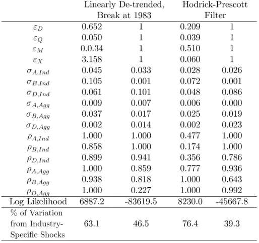
compute that less than half of the variation in output growth is due to industry-speci…c shocks. When I impose unitary elasticities of substitution on my model, I estimate a similar number for the aggregate importance of industry-speci…c shocks.2 In sum, these results indicate that sectoral shocks are more important than previously thought, and that the di¤erence is largely due to past papers’ imposition of a unitary elasticity of substitution between intermediate inputs and capital/labor. These results are robust to time period, industry classi…cation schemes, treatment of trends, and (for the most part) countries.
This paper resolves the hypothesis, …rst advanced in Long and Plosser (1983), that independent industry-speci…c shocks generate patterns characteristic of modern business cycles. Models of business cycles typically portray ‡uctuations as the result of economy-wide, aggregate disturbances to production technologies and preferences. These disturbances, however, are di¢ cult to justify independently, and may simply represent "a measure of our ignorance."3 Given the results of the current paper, future research on the sources of business cycle ‡uctuations would bene…t from moving beyond the predominant one-sector framework. 2See Section4.2for a discussion of why the numbers reported inFoerster, Sarte, and Watson (2011)may
di¤er from the estimates I provide here.
3This phrase was coined by Abramovitz (1956), when discussing the sources of long-run growth, but
applies to our understanding of short-run aggregate ‡uctuations, as well. More recently,Summers (1986) andCochrane (1994)have argued that it isa priori implausible that aggregate shocks can exist at the scale needed to engender the business cycle ‡uctuations that we observe.
1.1
Literature Review and Outline
The current paper falls within the literature on multi-industry real business cycle models, …rst introduced in Long and Plosser (1983). Long and Plosser present a model in which the economy is comprised of a collection of perfectly competitive industries. Each industry produces its output by employing a combination of capital, labor, and intermediate inputs. The capital and intermediate input bundles of each industry are, in turn, combinations of goods that are purchased from other industries. Long and Plosser (1983) and others in this literature (e.g., Horvath 1998,2000, Dupor 1999,Acemo¼glu et al. 2012, and Acemo¼glu, Özda¼glar, and Tahbaz-Salehi 2013) use this framework to argue that idiosyncratic shocks to industries’productivities, by themselves, have the potential to generate substantial aggregate ‡uctuations.4 These papers, however, do not allow for aggregate shocks; they are not
attempting to assess the relative importance of industry-speci…c and aggregate shocks.5
With an appreciation of this issue, Foerster, Sarte, and Watson (2011) present a methodology that allows them to recover the underlying productivity shocks from data on industries’ output growth. The authors perform a factor analysis on the recovered productivity shocks. They …nd that aggregate productivity shocks— the …rst two common factors from the factor analysis— represent most of the variation in the …rst part of their sample (1972 to 1983), and decline in volatility during the Great Moderation (1984 to 2007). As a result, industry-speci…c shocks account for 20% and 50% of the variation in industrial production during the two parts of their sample.
Compared to the Long and Plosser literature in general— and Foerster, Sarte, and Watson (2011) in particular— the current paper makes three advances, all of which are nec-essary to properly gauge the contribution of sectoral shocks to aggregate volatility. First, I examine the implications of industry-speci…c and aggregate shocks on other observable variables— industry level output prices and intermediate input purchases— that have up to now been ignored. To be able to compare data on prices and intermediate input purchases to their theoretical counterparts, I include non-technology shocks (namely, shocks to the preferences of the representative consumer over the industries’outputs). In the context of one-sector models, preference shocks account for a large portion of business cycle ‡uctuations, and thus should also be included in a multi-industry analysis.6 Second, I allow for ‡exible
4Within this literature,Dupor (1999)is somewhat unique: Instead of arguing that industry-speci…c shocks
have the potential to produce business cycle ‡uctuations, he does the converse: He provides conditions on the input-output matrix under which industry-speci…c shocks are irrelevant.
5Horvath (2000)includes aggregate shocks in his analysis, but does not attempt to estimate the relative
magnitudes of the aggregate and sectoral shocks.
6Although there is some contention on this point, technology shocks alone cannot explain most of the
business cycle variation of aggregate activity (see, for example, Galí and Rabanal 2004 and Smets and Wouters 2007for two analyses of one-sector economies).
substitution patterns in consumers’preferences and industries’production technologies. In particular, Foerster, Sarte, and Watson (2011)and earlier papers impose unitary elasticities of substitution in consumers’preferences (across the goods produced by each industry) and in industries’production functions (across inputs).7 In contrast, I estimate these elasticities.
Allowing for a non-unitary elasticity of substitution between intermediate inputs and other inputs turns out to be critical: With the unit elasticity assumption, the model substantially understates the relative importance of industry-speci…c shocks. Finally, I make a sequence of smaller advances: I allow for consumption good durability, consider a dataset that covers the entire economy,8 and examine data from several developed economies.9
The model is delineated in Section2. Section3introduces the three main datasets— the Bureau of Economic Analysis (BEA) Input-Output Table, the BEA Capital Flows Table, and Dale Jorgenson’s 35-industry KLEMS dataset— and discusses two patterns in the data which will guide the estimation. Section 4 describes the estimation procedure, the main empirical results, and a sensitivity analysis of the benchmark results. Section 5 contains a simple example, which provides intuition as to how the parameters are identi…ed and why allowing "Q to be freely estimated yields higher estimates of the relative importance of
sectoral shocks. Section 6 concludes.10
7Horvath (2000)accommodates non-unitary elasticities of substitution in consumers’preferences (across
goods) and in the production of the intermediate input bundle (across inputs purchased from upstream industries), but imposes a unitary elasticity of substitution among labor, capital, and the intermediate input bundle. As I argue in this paper, this last parameter is the most important. Another di¤erence between the current paper andHorvath (2000)is that the earlier paper does not attempt to estimate the values of these elasticities of substitution. Instead, he performs a sensitivity analysis of his results around his benchmark speci…cation (in which all of the aforementioned elasticities of substitution are equal to 1); see Section 5.2 of that paper.
8Foerster, Sarte, and Watson (2011) is unique in its application of the Federal Reserve Board’s dataset
on industrial production, a dataset that spans only the goods-producing sectors of the U.S. economy. Other papers (e.g.,Long and Plosser 1983andHorvath 2000), employ a dataset that covers the entire economy.
9Another line of research attempts to gauge the relative importance of industry-speci…c shocks by
esti-mating vector autoregressions (seeLong and Plosser 1987,Stockman 1988,Shea 2002, orHolly and Petrella 2012).
There are other explanations, in addition to the input-output-channel explanation, for the relevance of micro shocks. Gabaix (2011)demonstrates that individual …rms, because of their size, engender substantial aggregate ‡uctuations. Along these lines,Carvalho and Gabaix (2013) show that certain industries, those with particularly volatile productivities, account for an outsize fraction of aggregate volatility.
10Additional robustness checks related to Section 4’s results (AppendixA), details on the dataset
(Appen-dicesBandC), and ancillary calculations (AppendicesDandE) are all contained in the Appendix. Finally, in Appendix F, I exploit micro data from selected manufacturing industries to provide an alternative, cor-roboratory estimate of the elasticity of substitution between industries’ intermediate input purchases and their purchases of capital and labor.
2
Model
In this section, I present a multi-industry general equilibrium model, along the lines of
Long and Plosser (1983)andFoerster, Sarte, and Watson (2011). This is the simplest model that can be used to compare the importance of industry-speci…c and aggregate disturbances and to estimate the elasticities of substitution in preferences and production. The model is populated by a representative consumer and N perfectly competitive industries. I …rst describe the representative consumer’s preferences, then the production technology of each industry, and …nally the evolution of the exogeneous variables.
2.1
Preferences
The consumer has balanced-growth-consistent preferences over leisure and the services provided by the N di¤erent consumption goods.
The preferences of the consumer are given by the following utility function:
U = 1 X
t=0
t
8 < :Dt;Agg
N
X
J=1
J DtJ
! log
2 4
N
X
J=1
( J DtJ)
1
"D ( C
J CtJ)
"D 1
"D
! "D
"D 13
5 "LS
"LS + 1 N
X
J=1
LtJ
!"LS+1
"LS 9=
; . (1)
The demand parameters, J, re‡ect the time-invariant di¤erences in the importance
of industries’ goods in the consumer’s preferences. Preferences over each industry’s con-sumption good evolve stochastically, with an aggregate (Dt;Agg) and an industry-speci…c
component (DtJ). The aggregate component a¤ects each industry symmetrically, while the
industry-speci…c component a¤ects individual industries independently. CtJequals the stock
of durable goods when J is a durable-good-producing industry and equals the expenditures on good/service J otherwise. For durable goods, J, the evolution of the stock of each consumption good,CtJ, is given by
CtJ =Ct 1;J (1 CJ) + ~CtJ , (2)
where C~tJ equals the consumer’s new purchases on goodJ at timet and CJ parameterizes
the depreciation rate of goodJ. The elasticities of substitution parameterize how easily the representative consumer substitutes across the di¤erent consumption goods ("D) and how
responsive the consumer’s desired labor supply is to the prevailing wage ("LS).11
To see more clearly how the preference shocks operate, suppose for a moment that there are no durable goods so that CJ = 1 for all industries. LetPtJ denote the Lagrange
multiplier on the periodtgoods market clearing condition for goodJ (see Equation8below), and letPtdenote the ideal price index at timet.12 Take the …rst-order condition with respect
to consumption of good J at date t:
PtJ =Dt;Agg N
X
I=1
I DtI
!
( J DtJ)
1
"D (CtJ)
1
"D
PN
I=1( I DtI)
1
"D (CtI)"D
1
"D
.
After some manipulation, one can show that the utility function given in Equation 1
implies that the representative consumer has the following demand function for good J at date t:
CtJ = J DtJ Dt;Agg
PtJ
Pt
"D 1
Pt
.
The Ds thus act to shift the demand curve for goodJ at time t. The industry-speci…c component (DtJ) shifts only the demand for good J, while the aggregate component (Dt)
shifts all time-t demand curves. The same forces remain when some goods do not fully depreciate each period, just in a more opaque form.
2.2
Production and Market Clearing
Each industry produces a quantity (QtJ) of good J at datet using capital (KtJ), labor
(LtJ), and intermediate inputs (MtJ) according to the following constant-returns-to-scale
11Horvath (2000)andKim and Kim (2006)use a more ‡exible speci…cation regarding the disutility from
supplying labor. In their speci…cation, the second line of Equation1is replaced by
"LS
"LS+ 1 N
X
J=1
(LtJ) +1
! +1
"LS+1
"LS
:
The idea behind this speci…cation is to "capture some degree of sector speci…city to labor while not deviating from the representative consumer/worker assumption." Horvath (2000, p. 76) As it turns out, neither the volatility of aggregate economic activity nor the covariances of output across industries are particularly sensitive to the value of (see Table 9 of that paper). Moreover, since wages and hours are not among the observable variables that I am trying to match, the data that I employ in the following sections would have trouble identifying . For these reasons, I use the simpler speci…cation of the disutility from labor supply.
12The ideal price index is:
Pt
"N X
I=1
I DtI DtAgg
PN
J=1 J DtJ DtAgg
(PtI)1 "D
# 1 1 "D
production function:
QtJ = AtJ At;Agg (3)
2 6
4(1 J)
1
"Q KtJ
J
J B
tJ Bt;Agg LtJ
1 J
1 J!
"Q 1
"Q
+ ( J) 1
"Q (M
tJ)
"Q 1
"Q 3 7 5
"Q
"Q 1
.
The parameters J and J re‡ect long-run averages in each industry’s usage of
intermediate inputs, labor, and capital. These parameters will eventually be inferred from the factor cost shares of each industry. At;Agg AtJ and Bt;Agg BtJ are, respectively, the
factor-neutral and the labor-augmenting productivity of industry J at time t. As with the preference parameters, each of these productivity terms consists of an industry-speci…c component and a component that is common to all industries.
The parameter "Q dictates how easily factors of production are substituted. From
the cost-minimization condition of the industry J representative …rm, the relationship be-tween the intermediate input cost share of industryJand the industryJ speci…c intermediate input price (denoted Pmat
tJ ) is log-linear, with slope 1 "Q:13
log P
mat tJ MtJ
PtJ QtJ
= log J + (1 "Q) log
Pmat
tJ
PtJ
+ ("Q 1) log (AtJ At;Agg) . (4)
When "Q = 1, as assumed in previous papers, an industry’s intermediate input cost share
is constant, independent of the price of its intermediate inputs, a prediction that I will show to be at odds with the data.
The evolution of capital, for each industry J, is given in Equation5.
Kt+1;J = (1 K)KtJ+XtJ . (5)
The capital stock is augmented via an industry-speci…c investment good, XtJ, and
de-13The equivalence between sales and costs in the denominator of the left-hand side of Equation4 comes
from the assumption that each industry is perfectly competitive, with a constant returns-to-scale production function.
To derive Equation 4, take …rst-order conditions of Equation 3 with respect to intermediate input pur-chases:
PtJmat = PtJ
@QtJ
@MtJ
= PtJ (AtJ At;Agg)
"Q 1
"Q (M
tJ) 1
"Q (
J QtJ) 1
"Q .
PtJmat "Q
= (PtJ)"Q(AtJ At;Agg)"Q 1(MtJ) 1 J QtJ .
preciates at a rate K that is common across industries.
The industry-speci…c investment good is produced by combining the goods produced by other industries. The X
IJ indicate how important industryI is in the production of the
industry J speci…c investment good, while"X parameterizes the substitutability of di¤erent
inputs in the production of each industry’s investment bundle:
XtJ =
N
X
I=1
X IJ
1
"X (X
t;I!J)
"X 1
"X
! "X
"X 1
. (6)
Analogously, the intermediate input bundle of industry J is produced through a combination of the goods purchased from other industries:
MtJ =
N
X
I=1
M IJ
1
"M (M
t;I!J)
"M 1
"M
! "M
"M 1
. (7)
In Equation 7,"M parameterizes the substitutability of di¤erent goods in the production
of each industry’s intermediate input bundle. The M
IJ indicate how important industry I
is in the production of the industry J speci…c intermediate input.
To emphasize, the parameters MIJ, XIJ, J, and J are time invariant. As such,
movements in the share ofJ’s expenditures spent on di¤erent factors of production are due, only, to the shocks to industries’productivity and consumers’preferences.
Finally, the market-clearing condition for each industry states that output can be used for consumption, as an intermediate input, or to increase one of the N capital stocks:
QtI =CtI (1 CI)Ct 1;I +
N
X
J=1
(Mt;I!J +Xt;I!J) . (8)
2.3
Evolution of the Exogeneous Variables
The three sets of exogenous variables— to factor-neutral productivity, labor-augmenting productivity, and preferences— follow stochastic processes each of a similar form. Each variable has an industry-speci…c and an aggregate component, both of which follow a …rst-order autoregressive process.
The industry-speci…c components take the form described by Equations 9to 11:
logAt+1;J = A;Ind logAtJ + A;Ind !Ind;AtJ . (9)
logBt+1;J = B;Ind logBtJ + B;Ind ! Ind;B
tJ . (10)
The aggregate components take the form characterized by Equations 12to 14:
logAt+1Agg = A;Agg logAt Agg+ A:Agg ! Agg;A
t . (12)
logBt+1Agg = B:Agg logBt Agg+ B;Agg !Agg;Bt . (13)
logDt+1;Agg = D;Agg logDt;Agg+ D:Agg !Agg;Dt . (14)
In Equations 9 to14, the !s are independent standard normal random variables.
Several assumptions are embedded within Equations 9to14. First, the persistence and standard deviations of each of the industry-speci…c components is assumed to be the same for all industries (e.g., Ind;D and Ind;D are common across all industries.) In reality,
industries may di¤er in how persistent and volatile their productivity and demand are. Moro (2012)andCarvalho and Gabaix (2013), for example, argue that productivity is substantially more volatile in manufacturing and …nance than in other industries. Second, Equations9to
14place strong restrictions on the covariance matrix of the productivities (or the covariance matrices of preferences) across industries. For example, the correlation between the produc-tivity growth of two industries is the same for all pairs.14 Despite their restrictive nature, the assumptions embedded in Equations 9 to14 are useful: they yield a parsimonious com-parison of the importance of the industry-speci…c and aggregate components of the shocks to the exogeneous variables.15
3
Data and Descriptive Statistics
The three datasets employed to evaluate the model are Dale Jorgenson’s 35-Sector KLEMS database, the 1992 BEA Input-Output Table, and the 1992 BEA Capital Flows Table. The …rst dataset is used to measure ‡uctuations in sales, inputs, and prices, while the second and third datasets are employed to measure long-run ‡ows of inputs across pairs of industries. I describe the three databases, in turn. Additional details can be found in AppendixB.
Dale Jorgenson’s 35-Sector KLEMS dataset contains information on industries’pro-14The growth of industryJ’s factor-neutral productivity equals:
log At+1;J At+1;Agg
AtJ At ;Agg
= A;Agg 1 logAt ;Agg+ A;Ind 1 logAtJ+ A;Ind !Ind;AtJ + A;Agg !Agg;At .
Thus, conditional on the productivities of industriesJ andJ0at timet, the correlation of the factor-neutral productivity growth of the two industries equalsh1 + ( A;Ind A;Agg)2
i 1
.
duction and input usage patterns at an annual level, from 1960 to 2005.16 As its name suggests, the dataset contains information on 35 industries, roughly at the 2-digit level for the manufacturing sector and at the 1 to 2-digit level for other sectors. I drop the "Gov-ernment Enterprises" industry, leaving 34 industries in my dataset. There are two main advantages of this dataset, compared to others that track industries’production ‡uctuations. First, unlike the NBER— CES Manufacturing database or the Federal Reserve Board’s In-dustrial Production database, Dale Jorgenson’s dataset contains information on the entire economy, not just the goods-producing sectors. Second, unlike the Industrial Production database, the dataset that I am working with tracks intermediate input prices and purchases for each industry. These data are critical in evaluating the shape of industries’production technologies.
The BEA Input-Output Table and Capital Flows Table provide information on the ‡ows of intermediate inputs and capital goods, across pairs of industries. While these data are published every …ve years, I use only the 1992 version of the two tables. By taking only one vintage of the Input-Output and Capital Flows Tables, I am assuming that the strength of the linkages across industries (as parameterized by the M
IJs and XIJs) are unchanged
throughout the sample period.
The four industry-level time series that I consider are gross output (YtI),17 the
inter-mediate input expenditure share (MtIshare), the price for the good produced by the industry (PtI), and the price for the intermediate input used by the industry (PtImat). Gross output is
the product of the industry output price (PtI) and the quantity of the good produced (QtI).
I compute the intermediate input expenditure share by taking the ratio of expenditures on intermediate inputs to the total expenditure on capital goods, labor, and intermediate inputs.
I perform three transformations on the variables of interest, with the aim of har-monizing the data and Section 2’s model. First, I consider growth rates of each of the variables, with the aggregate price level subtracted o¤ of the sales, output price, and input price measures.18 To mitigate the e¤ect of outliers on the parameter estimates, I winsorize the variables at the top and bottom 0:5 percentiles.19 Finally, because there is no trend 16KLEMS is an acronym for capital, labor, energy, materials, and services. The data can be found on
Dale Jorgenson’s home page (see http://scholar.harvard.edu/jorgenson/data).
17I will use the terms gross output and sales interchangeably.
18The rationale for subtracting the aggregate price level stems from Section2’s model’s omission of
mon-etary considerations. Because this model is not equipped to distinguish between technology growth from money supply growth as the source of aggregate price ‡uctuations, I have decided to simply remove aggregate price variation from the data. In the estimation stage, I also construct the model counterpart to changes in the aggregate price level and subtract this series from industries’sales and price measures.
19When winsorizing, I pool across all industries, compute the growth rate of the variable of interest across
present in the model, I linearly de-trend the four industry level variables.20 Throughout this section and the next two, I use v to refer to the transformed version of variable V.
Having introduced the data sources and discussed the industry de…nitions, I now present two patterns which will guide the empirical analysis of Section4. The …rst pattern is simply that activity is correlated across industries. Over the 352 pairs of industries, the
correlation of industries’ sales growth rates is, on average, 27:3%. The correlation of the growth rates of industries’intermediate input cost shares is 22:2% for the average industry pair. As discussed in the introduction, there are two possible explanations for the positive values of these correlations. Aggregate events— such as a change in monetary or …scal policy or a …nancial crisis— no doubt play some role in explaining these co-movements. At the same time, because of the input-output relationships that exist between industries, pairs of industries’sales (or input purchases) will co-move even with independent, industry-speci…c shocks. Disentangling the two alternatives is the primary goal of the model. In general, the estimation will assign greater importance to aggregate (versus industry-speci…c) shocks the higher the value of the cross-industry correlations.
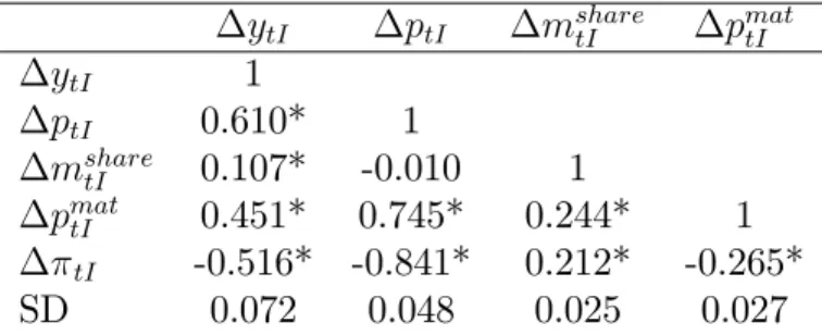
Table 1 presents the second set of patterns: the volatility and average correlations in the growth rates of the four level characteristics, now pooled across all industry-years. Here, the standard deviation of the growth rate of gross output is 7:2% in the pooled sample. Output and input prices are less volatile: The standard deviations of the growth of the price variables are 4:8% and 2:7%, respectively. Finally, the intermediate input cost share is the least volatile. Critically, however, the cost share ‡uctuates over time and is positively correlated with input prices. The ‡uctuating intermediate input cost share is a …rst indication that sectoral production technologies are not well-described by a Cobb-Douglas production function.
Motivated by Equation 4, de…ne tI pmattI ptI as the change in the ratio
of industry I’s intermediate input price to its output price. According to Equation 4, the strength and direction of the relationship between msharetI and tI depends critically on
AppendixA, I consider the e¤ect of varying this0:5%cut-o¤ to 0:25% or1:0%.
20In estimations of dynamic general equilibrium models, the choice of the de-trending procedure is
poten-tially important; see Canova (2013). In Appendix A, I re-estimate the model with alternative de-trending procedures. Both the relative importance of industry-speci…c shocks and the estimate of"Q are robust to
the alternative procedures.
An alternative— intuitively appealing but unfortunately infeasible— way to deal with trends would be to include both transitory and permanent shocks in the model. This would obviate the need to de-trend the data before estimation; the parameters governing the permanent and transitory shock processes would be jointly estimated in a single stage. I do not pursue this approach, mainly because of the di¢ culty of scaling the model by the permanent shocks. Doing so requires a clean characterization of the changes in the industry-level observable variables as functions of the permanent shocks, something that exists only for a few special cases of the model (such special cases can be found in, for example,Ngai and Pissarides 2007andAcemo¼glu and Guerreri 2008).
ytI ptI msharetI pmattI
ytI 1
ptI 0.610* 1
mshare
tI 0.107* -0.010 1
pmattI 0.451* 0.745* 0.244* 1
tI -0.516* -0.841* 0.212* -0.265*
SD 0.072 0.048 0.025 0.027
Table 1: Correlations and standard deviations of the growth rates of industry-level statistics.
Notes: Stars indicate that the correlation is statistically di¤erent from0, at the 5%level.
"Q. The positive, 21%, correlation between tI and msharetI indicates that the elasticity
of substitution between intermediate inputs and other inputs may be less than 1. The intermediate input cost share and the relative price of intermediate inputs are positively related over longer horizons, as well: The correlation between msharetI and tI equals9:1%,
25:0%, and 37:5%, over 3-year, 5-year, and 10-year intervals, respectively, thus indicating that the low substitutability between intermediate inputs and other inputs is not just a short-run phenomenon.
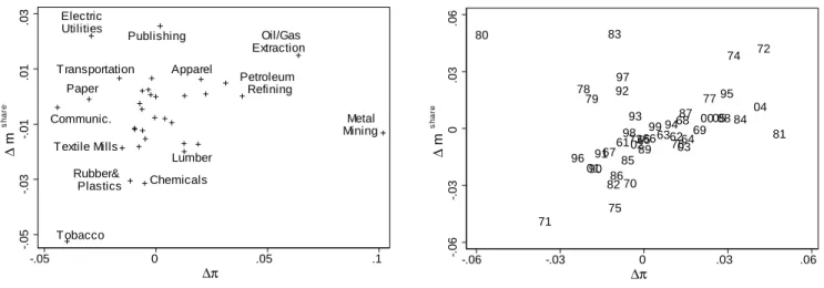
As I will argue below in Sections 4 and 5, the estimate of "Q both hinges on the
relationship between tI and msharetI and is a crucial component in an assessment of
the relative importance of industry-speci…c shocks. For these reasons, it will be useful to examine the correlation between tI and msharetI in more detail. Figure 1 depicts the
cross-sectional (left panel) and time series (right panel) relationships between these variables. In the left panel, I plot tI and msharetI for a typical year, 1984: In this year the correlation
equals 18%. The right panel plots msharetI and tI for a single industry, Miscellaneous
Manufacturing, across the entire 45-year sample period. For this industry, input prices increased substantially between 1971 and 1974.21 During this time, the intermediate input
cost share increased moderately, as well, from 48% to52% of total expenditures.
Were it not for the omitted variable of industry J productivity (the …nal term on the right-hand side), Equation 4 would yield an unbiased estimate of "Q: I would
sim-ply need to compute the slope of the relationship between log (Pmat
tJ PtJ) and industries’
log (MtJ). However, because industries’ productivities and output prices are (negatively)
correlated, such an exercise would yield a biased estimate of "Q. The exercise to which I
now turn— jointly estimating the preference and technology elasticities in conjunction with the parameters of the exogeneous productivity and demand processes— circumvents these problems.
21During this period there was a broad increase in commodity prices. SeeCooper and Lawrence (1975)
Tobacco Rubber&
Plastics Chemicals Electric
Utilities
Publishing
Textile Mills
Oil/Gas Extraction
Metal Mining Petroleum
Refining Communic.
Apparel
Lumber Transportation
Paper
-.05
-.03
-.01
.01
.03
∆
m
s
h
a
re
-.05 0 .05 .1
∆π
80
71 96
78 79
0190 9167
82 83
75 86 92
61 97
85 98
70 93 730265
8966 99
639462 76 68 03 87
6469 00
77 0588
95 74
84 04
72
81
-.06
-.03
0
.03
.06
∆
m
s
h
a
re
-.06 -.03 0 .03 .06
∆π
Figure 1: Relationship between mshare and .
Notes: Left panel: Data from 1984. Right panel: Data from the Miscellaneous Manufacturing industry.
4
Estimation and Results
This section contains the main empirical content of the paper. In this section, I describe the estimation procedure (Section4.1), present the model’s MLE estimates and correspond-ing variance decompositions (Section 4.2), and examine the sensitivity of the benchmark results to changes in sample, industry de…nition, period length, country, and other details of the estimation procedure (Section 4.3).
4.1
Estimation Procedure
I apply a combination of moment matching and maximum likelihood to empirically evaluate the model.
The parameters J, J, J, XIJ, and MIJ are chosen to match the model-predicted
cost shares to the corresponding values in the data. These parameters contain only infor-mation about the steady-state of the equilibrium allocation. The demand shares, J, are chosen so that the model’s steady-state consumption choices are proportional to the amount that the industry sells; the J are restricted to sum to 1. The other parameters are chosen to match factor intensities, for each industry-factor pair. For instance, J is the value that equates the model-predicted intermediate input cost share with the empirical counterpart.22
The empirical values that are used to calibrate the factor intensities are described in Ap-22When"
Q = 1, the intermediate input cost share and J are equal to one another. Alternatively, when
intermediate inputs are gross complements or gross substitutes to other factors of production, the model-predicted cost share will also depend on the relative prices of the intermediate input bundle and the price of the other factors of production.
pendix B. Appendix D.2 provides additional details on the calibration of the parameters relevant to the steady state.23
I choose , K, CJ, and "LS based on the values used in past analyses. I set
the discount factor, , to 0:96 and the capital good depreciation rate, K, to 0:10. The
durable good depreciation rates, CJ, are taken from computations published by the BEA
(see Appendix B for these depreciation rates). In the benchmark calculations, I set the Frisch labor supply elasticity to be equal to 1, in line withPrescott (2006). In the appendix, I re-estimate the model using larger values for "LS, closer to the values given in Chetty et
al. (2011).
The other parameters— the elasticities of substitution and the parameters charac-terizing the exogeneous processes— are estimated via maximum likelihood. The maximum likelihood procedure compares the model’s predictions over the growth rates of industries’ sales, prices, and intermediate input cost shares to their data counterparts.24
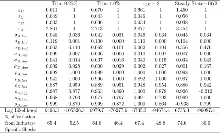
I allow for measurement error in industries’intermediate input cost shares. There is considerable evidence that the values of industries’ intermediate inputs are measured with error, and that this measurement error is more severe than for the other variables. First, as Jorgenson, Gollop, and Fraumeni (1987) write in their description of the KLEMS dataset, information on industries’intermediate input purchases are, in general, taken as a residual of the gross output of a given industry and the labor and capital value added of that industry (see p. 159). Any measurement error in labor or capital inputs will show up in the intermediate input cost shares, as well. For manufacturing industries, it is possible to gauge the extent to which intermediate input cost shares are mismeasured in the Jorgenson KLEMS Dataset. The NBER— CES manufacturing dataset, which draws on data from the Census Bureau’s Annual Survey of Manufacturers, is an alternate source of information on industry level sales, prices, and input cost shares. Applying the same industry classi…cation and using the same sample period as in the current paper, I compute that the standard deviation of the growth rate of industries’intermediate input cost shares is1:8%for the NBER— CES dataset and 2:1% for the Jorgenson KLEMS dataset. Since these two datasets measure the same thing, the di¤erence in these standard deviations serves as a lower bound for the 23In AppendixA, I examine the sensitivity of Section4’s results to using 1972, instead of 1992, as the year
to which the steady-state allocation is calibrated.
24All computations are performed in Dynare. The value of the likelihood function, at any parameter
con…guration, is the result of the Kalman …lter algorithm applied to the …rst-order approximation to the model introduced in Section 2. Regarding the Kalman …lter, seeCanova (2007, Chapter 6) for a textbook introduction, and Adjeman et al. (2011) for a description of the practical implementation. To …nd the numerical maximum of the log likelihood function, I use a simplex search algorithm, and try di¤erent starting points to check that the search algorithm is …nding a global optimum.
measurement error present in the Jorgenson KLEMS dataset.
The measurement errors serve a second, more practical, role in the empirical analy-sis. Without these measurement errors, speci…cations in which "Q is restricted to 1cannot
possibly be estimated with the aforementioned procedure. With a unitary elasticity of sub-stitution between intermediate inputs and value added, the intermediate input cost share must be constant. Thus, when"Q equals1, the log likelihood would be negative in…nity for
all combinations of the other parameters.
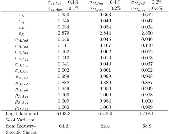
In the benchmark calculations, I assume that the measurement error for each in-dustry has an inin-dustry-speci…c and an aggregate component (call these MtJerror and Mt;Aggerror, respectively). Thus, the observed intermediate input cost share is speci…ed by the following equation:
MtJshare P
mat tJ MtJ
YtJ
MtJerror Mt;Aggerror . (15) The logarithm of each component of an industry’s measurement error follows an …rst-order autoregressive process, with a serial autocorrelation of0:8and innovations that have a standard deviation of0:2%.25 I choose these values to be roughly consistent with the evidence
described above and to allow the productivity and demand shocks to explain almost all of the variation in industries’intermediate input purchases.
4.2
Results
Parameter estimates are collected in Table 2.
The full speci…cation is presented in the …rst column. The …rst four rows give the estimates of the elasticities of substitution; the next six rows give the estimates of the standard deviations of the innovations to productivities and preferences; and the …nal six give the estimates of the serial autocorrelations of the exogeneous processes. The estimate for the elasticity of substitution, "Q, between intermediate inputs and value added is 0:05;
intermediate inputs and value added are used in (almost) …xed proportions. The elasticity of substitution,"D, in consumer’s preferences, is0:65, indicating the the goods produced by
di¤erent industries are also gross complements. Finally the elasticity of substitution in the production of the intermediate input bundle, "M, is close to 0.
In columns (2) to (6), I restrict various combinations of the elasticities of substitution to be equal to1. The point of this exercise is to understand the impact of the assumptions made by previous authors, such as Foerster, Sarte, and Watson (2011)and Acemo¼glu et al. (2012), regarding these elasticities of substitution. The largest drop in the log likelihood 25In AppendixA, I show that the results of the current section are robust to moderate changes to
Speci…cation (1) (2) (3) (4) (5) (6)
"D 0.654 1 1 0.587 1 1
"Q 0.046 0.053 0.020 1 1 1
"M 0.034 0.031 1 0.128 0.010 1
"X 2.870 0.001 1 2.313 0.731 1
A;Ind 0.046 0.045 0.042 0.034 0.035 0.034 B;Ind 0.110 0.113 0.110 0.000 0.000 0.000 D;Ind 0.062 0.072 0.103 0.061 0.071 0.105 A;Agg 0.010 0.000 0.008 0.010 0.009 0.007 B;Agg 0.040 0.038 0.040 0.001 0.016 0.015 D;Agg 0.001 0.006 0.000 0.050 0.001 0.021 A;Ind 1.000 0.981 1.000 1.000 1.000 1.000 B;Ind 0.889 0.937 0.894 1.000 1.000 0.999 D;Ind 0.949 0.944 0.957 0.964 0.933 0.956 A;Agg 1.000 0.552 0.934 1.000 0.860 0.850 B;Agg 0.984 0.973 0.962 0.978 1.000 0.781 D;Agg 1.000 -0.257 1.000 0.964 1.000 1.000
Log Likelihood 6743.0 6682.1 6397.6 -94288.6 -94374.2 -94677.1 Table 2: MLE Estimates.
Notes: Each column gives the results from a di¤erent speci…cation. Whenever a "1" appears in the …rst four rows, the corresponding elasticity is set equal to1prior to estimating the other parameters. 26
function occurs in speci…cations for which "Q is …xed at 1: The model simply cannot …t
movements in industries’intermediate input cost shares. Imposing "Q = 1 also alters the
estimated values of the exogeneous processes. Most importantly, the estimated value B;Ind
is considerably larger in the …rst three columns.
The estimates of "Q and "D given in Table 2 broadly accord with the few existing
estimates for these parameters, with "Q on the lower end of existing estimates. With
respect to the estimate of "D, the most appropriate comparison would probably be Ngai
and Pissarides (2007)and its cited sources. The authors argue that the "observed positive correlation between employment growth and relative price in‡ation across two-digit sectors" (p. 430) is consistent with an estimate of "D that is less than 1.27 Bruno (1984) estimates
"Q by running an industry panel regression of manufacturing industries’intermediate input
26Standard errors are omitted to preserve space. These standard errors are almost universally small, on
the order of1%or less.
27To emphasize,"
D parameterizes how easily the consumer can substitute across coarsely-de…ned
indus-tries’ products (for example the elasticity of substitution between automobiles and furniture, or between apparel and construction). Broda and Weinstein (2006) and Foster, Haltiwanger, and Syverson (2008), among others, estimate a much lager elasticity of substitution in consumers’preferences. These larger elas-ticities of substitution are estimated usingwithin-industry variation, and characterize how easily consumers substitute between, for example, ready-mix concrete produced by two di¤erent plants, or between di¤erent varieties of red wine.
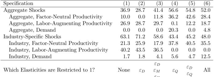
Speci…cation (1) (2) (3) (4) (5) (6)
Aggregate Shocks 36.9 28.7 41.4 56.6 54.8 52.0
Aggregate, Factor-Neutral Productivity 10.0 0.0 11.8 36.2 42.6 28.4 Aggregate, Labor-Augmenting Productivity 26.9 28.7 29.7 0.1 12.2 18.7
Aggregate, Demand 0.0 0.0 0.0 20.3 0.0 4.8
Industry-Speci…c Shocks 63.1 71.2 58.6 43.4 45.2 48.0 Industry, Factor-Neutral Productivity 21.3 25.9 17.9 37.8 40.5 35.5 Industry, Labor-Augmenting Productivity 40.2 43.5 36.5 0.0 0.0 0.0
Industry, Demand 1.7 1.8 4.1 5.6 4.7 12.5
Which Elasticities are Restricted to 1? None "D
"D
"M
"X
"Q
"D
"Q
All
Table 3: Variance Decompositions.
Notes: Each row gives the fraction of the variance in aggregate output growth that is due to the speci…ed type of shock. The columns correspond to the speci…cations estimated in Table2.
expenditure shares against the relative price of intermediate inputs. Bruno’s benchmark speci…cation yields an estimate of "Q = 0:3; other speci…cations in this paper have "Q
estimated to be anywhere in the range of 0:2 to 0:9. Rotemberg and Woodford (1996)
run a similar regression, but instrument the relative price of intermediate inputs using the price of crude oil. For industries within the manufacturing sector, Rotemberg and Woodford estimate that"Q= 0:7.
Table 3 presents the forecast error variance decompositions. The table apportions the fraction of the variance of the change in aggregate output that is due to these six sets of shocks. In the unrestricted speci…cation, industry-speci…c demand, factor-neutral pro-ductivity, and labor-augmenting productivity shocks account, respectively, for2%,21%, and
40% of aggregate output growth variation, meaning that 63% of the variability of aggre-gate output growth originates from industry-speci…c shocks; see column 1. Restricting
"Q = 1, as I do in the fourth, …fth, and sixth columns of Table 3, decreases the estimated
importance of industry-speci…c shocks to approximately 43% to 48%, close to the values reported by Foerster, Sarte, and Watson (2011). (As a reminder, the authors impose that
"Q ="D ="M ="X = 1.) In that paper, the authors report that approximately40% of the
variability of industrial production growth is due to industry-speci…c shocks.28
28Foerster, Sarte, and Watson (2011)perform a factor analysis on industries’productivity shocks and then
compute the fraction of industrial production growth that is due to the …rst two factors. The remaining variation can be considered equivalent to the industry-speci…c productivity shocks in the current paper. The two common factors explain80%of the variation in overall industrial production growth in the …rst third of the sample (1972 to 1983) and50% in the latter two-thirds (1984 to 2007).
There are a few potential explanations for the di¤erence. The biggest di¤erence is that the Foerster, Sarte, and Watson (2011)analysis is restricted to the goods-producing sectors of the economy, while I study the entire private economy. Other di¤erences include a di¤erence in sample period (1960 to 2005 in the
Tables 2 and 3 contain the main results of the paper. The remainder of the paper is devoted to studying the robustness of the MLE estimates, explaining how the elasticities of substitution are identi…ed, and discussing a simple example that explains why freely estimating"Q corresponds to larger estimates for the relative importance of industry-speci…c
shocks.
4.3
Robustness Checks
Industry De…nition, Sample Period, and Period Length
Table 4considers three robustness checks: to the industry classi…cation scheme, to the sample period, and to the period length. Throughout the remainder of the section, I consider two speci…cations: In the …rst, all elasticities are freely estimated, while the second sets all elasticities equal to 1 (corresponding to columns 1 and 6 of Table 2). The motivation for presenting both speci…cations is to establish the impact of trying to …t the data on industries’ intermediate input cost shares, something that is only possible when "Q 6= 1.
In the …rst two columns, I establish that the results of Tables2and3are qualitatively robust to an 8-industry partition of the economy.29 The relative importance of
industry-speci…c shocks is now somewhat larger than in the benchmark industry-speci…cation, representing
71% of the variation in aggregate output growth. The primary di¤erence, compared to the benchmark speci…cation, is that the demand and productivity processes are substantially less volatile. This di¤erence re‡ects the "averaging-out" of the idiosyncratic shocks within each of the 8 coarsely-de…ned industries.
Columns 3 through 6 examine the sample period stability of the parameter estimates. Consistent with the large literature on the Great Moderation, the estimated standard de-viations are smaller in the second half of the sample period. The decline in dispersion is attributable mainly to the decline of aggregate shocks, similar toFoerster, Sarte, and Watson (2011): The fraction of variability due to industry-speci…c shocks is60%in 1960 to 1982 and
70% in 1983 to 2005.
In the …nal columns, I re-estimate the model using biennial data. The motivation behind this exercise is to examine whether the low values of"Q or"M are due to adjustment
current paper, compared to 1972 to 2008 in Foerster, Sarte, and Watson 2011), period length (one quarter in Foerster, Sarte, and Watson 2011 versus one year, here), my inclusion of shocks to demand, which are absent inFoerster, Sarte, and Watson (2011), and Foerster, Sarte, and Watson (2011)’s imposition of unit roots in the stochastic process governing the productivity of each industry.
29These industries are primary inputs (industries 1 to 5, according to Table11), construction (industry 6),
non-durable goods (industries 7 to 10 and 13 to 18), durable goods (industries 11, 12, and 19 to 27), transport (industries 28 to 31), wholesale and retail (industry 32), …nance, insurance, and real estate (industry 33), and personal and business services (industry 34). While it would be interesting to test the sensitivity of these results to a …ner industry classi…cation scheme, the necessary data are unavailable.
Coarse Industry
De…nition 1960-1982 1983-2005
Period Length= 2 Years
"D 0.812 1 0.749 1 0.616 1 0.579 1
"Q 0.020 1 0.055 1 0.063 1 0.031 1
"M 0.030 1 0.0.37 1 0.034 1 0.033 1
"X 0.061 1 0.364 1 1.628 1 2.953 1
A;Ind 0.029 0.023 0.045 0.035 0.044 0.031 0.067 0.050 B;Ind 0.055 0.014 0.105 0.000 0.110 0.000 0.166 0.001 D;Ind 0.038 0.045 0.069 0.106 0.055 0.098 0.100 0.173 A;Agg 0.000 0.005 0.010 0.009 0.007 0.002 0.016 0.014 B;Agg 0.020 0.009 0.033 0.023 0.041 0.019 0.068 0.041 D;Agg 0.017 0.023 0.017 0.001 0.000 0.025 0.000 0.007 A;Ind 0.948 1.000 0.986 1.000 0.954 1.000 0.918 0.977 B;Ind 0.888 0.211 0.902 1.000 0.821 -0.990 0.769 0.654 D;Ind 0.942 1.000 0.797 0.887 0.999 1.000 0.912 0.920 A;Agg 0.357 0.874 0.999 0.807 0.999 1.000 0.864 1.000 B;Agg 0.301 0.999 0.824 0.727 0.999 1.000 0.896 1.000 D;Agg 0.471 1.000 0.931 1.000 0.999 0.422 0.999 1.000
Log Likelihood 1975.3 -8106.8 3145.9 -48565.7 3543.5 -35526.4 2486.8 -20266.3 % of Variation
from Industry-Speci…c Shocks
70.7 64.8 60.2 32.2 69.6 72.2 55.8 45.0
Table 4: MLE Estimates, Robustness Checks: Industry De…nition, Sample Period, and Period Length.
Notes: The …nal row gives the fraction of aggregate output growth volatility that is due to industry-speci…c demand and productivity shocks.
costs— or some other friction— that prevent industries from substituting across its factors of production in the very short run. To the extent that this is the case, the results in the …nal columns of Table 4 should di¤er from those in the benchmark speci…cation. It turns out that the change in period length alters neither the relative importance of industry-speci…c shocks nor the estimates of "Q or "M. The primary di¤erence between these speci…cations
are larger values for the standard deviations of the productivity and demand shocks, and a smaller estimate of the preference elasticity of substitution ("D).
Which Shocks Should the Estimation Include?
It is possible that other disturbances— in addition to, or perhaps instead of, shocks to demand or productivity— drive movements in industries’ sales, prices, and intermediate
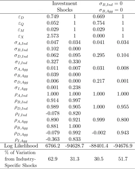
input cost shares.30 Here, I explore the e¤ects of the addition and deletion of sources of variation on the model’s estimates.
Investment Shocks
B;Ind = 0 B;Agg = 0
"D 0.749 1 0.669 1
"Q 0.052 1 0.754 1
"M 0.029 1 0.029 1
"X 2.573 1 0.000 1
A;Ind 0.047 0.034 0.041 0.034 B;Ind 0.102 0.000
D;Ind 0.062 0.095 0.295 0.104 I;Ind 0.327 0.330
A;Agg 0.011 0.007 0.031 0.008 B;Agg 0.039 0.000
D;Agg 0.006 0.000 0.217 0.001 I;Agg 0.001 0.238
A;Ind 1.000 1.000 1.000 1.000 B;Ind 0.914 0.997
D;Ind 0.989 0.905 1.000 0.955 I;Ind -0.078 0.820
A;Agg 0.890 0.921 0.999 0.800 B;Agg 0.881 1.000
D;Agg -0.079 0.992 -0.002 0.943 I;Agg -0.363 0.833
Log Likelihood 6766.2 -94628.7 -88401.4 -94676.9 % of Variation
from Industry-Speci…c Shocks
62.9 31.3 30.5 51.7
Table 5: MLE Estimates, Robustness Checks: Di¤erent Sets of Shocks.
Notes: The …nal row gives the fraction of aggregate output growth volatility that is due to industry-speci…c demand and productivity shocks.
Analyses of one-sector economies indicate that investment-speci…c technology shocks account for a large fraction of the business cycle variation in output and (see Fisher 2006
and Justiniano, Primiceri, and Tambalotti 2010). In the context of the model presented in Section2, I alter Equation 5 to include shocks to the investment technology:
Kt+1;J = (1 K) KtJ+ tJ t;Agg XtJ . (16)
30Canova, Ferroni, and Matthes (2013, Section 4)show that parameter estimates can be sensitive to the
choice of shocks and observable variables used in the estimation procedure. Guerron-Quintana (2010)and Ríos-Rull et al. (2012)make a similar point.
In Equation 16, tJ and t;Agg are industry-speci…c and aggregate investment technology
shocks. These shocks alter the e¢ ciency by which an industry’s investment good is trans-formed into its next-period capital stock. As with the other stochastic processes, assume that thelog tJ and log t;Agg are each …rst-order autoregressive processes.
Including investment shocks alters neither the estimated relative importance of industry-speci…c shocks nor the estimates of the model’s elasticities of substitution (see the …rst two columns of Table5). These shocks are, however, moderately important, representing
22% of output volatility. There are two potential explanations why investment shocks play a less prominent role here than in toFisher (2006)or Justiniano, Primiceri, and Tambalotti (2010). First,Justiniano, Primiceri, and Tambalotti (2010)show that investment shocks are particularly important in models that also incorporate price and wage stickiness. Their ab-sence in the model of Section2may account for the discrepancy between my multi-industry model and results from one-sector models. Second, it is possible that the mere consid-eration of a model of multiple industries may reduce the scope of investment technology shocks. As in the one-sector models, investment shocks alter the relative price of capital goods. Unlike these models, however, productivity shocks to the few capital-producing industries— Construction, Non-electrical Machinery, Electrical Machinery, and Transporta-tion Equipment— will have a similar e¤ect on the relative price of capital goods. While the reason behind the limited importance of investment shocks may be unclear, it is clear that industry-speci…c shocks are the predominant source of aggregate ‡uctuations, as in the benchmark speci…cation.
In columns 3 and 4, I remove the labor-augmenting productivity shocks (Bt;Agg and
theBtJs) as a source of variation. The main goal of this exercise is to show why the
labor-augmenting productivity shocks are included in the benchmark speci…cation in the …rst place: Without these shocks, the model cannot possibly match the dynamics of industries’ intermediate input purchases (compare the log likelihood of column 3 to that given in the …rst column of Table 2).31 The B shocks alter the marginal product of labor and thus alter the relative marginal productivity of intermediate inputs to other inputs. In turn, these B shocks drive much of the variation in industries’ intermediate input cost shares. A secondary goal of this exercise is to provide an example (albeit a dubious one) in which aggregate shocks explain the bulk, roughly 70%; of GDP growth variation. It turns out that only aggregate shocks, and not industry-speci…c shocks, can account for the volatile intermediate input cost shares that are observed in the data when B;Agg = B;Ind = 0. I
31I experimented with several other speci…cations that also omitted labor-augmenting productivity shocks
as a potential source of variation, and always found that the maximized likelihood was several orders of magnitude smaller than the maximum of the benchmark speci…cation.
explain why this is the case, using a simple example, in Section 5.1.
International Evidence
Table 6 presents results from estimations involving data from other countries. For all countries, "Q is less than 0:15, and always signi…cantly less than 1: With the exception
of Italy, industry-speci…c shocks account for the bulk of the variation in aggregate output growth.
Similar to the United States, restricting"Q = 1diminishes the relative importance of
these shocks for three of the countries in the sample: Denmark, the Netherlands, and Spain. For the other three countries (France, Italy, and Japan), the restricted speci…cation has a more prominent estimated role for industry-speci…c shocks. In the data, the distinguishing features of these two sets of countries are the cross-industry correlation of industries’sales and the cross-industry correlation of industries’ intermediate input cost shares. In the restricted speci…cation, intermediate input cost shares are uninformative about the model’s parameters. For countries that have highly correlated sales, across industries, aggregate shocks will explain most of the output variation. When"Q is freely estimated, intermediate
input cost shares will also now inform the estimates of the stochastic productivity and demand processes. All things equal, the speci…cation with estimated "Q will indicate that
industry-speci…c shocks are relatively more important for the countries for which sales are highly correlated and intermediate input cost shares are uncorrelated.32
In summation, industry-speci…c shocks are the primary source of aggregate ‡uc-tuations for most, but not all, countries. Including intermediate input cost shares as an observable variable, only possible when"Qis freely estimated, increases the estimated
impor-tance of industry-speci…c shocks for countries with uncorrelated intermediate input growth rates, and decreases the estimated importance of micro shocks for the remaining countries.
32To provide some support for this argument, consider the relationship between the following two variables.
The …rst variable is the di¤erence, across the free and restricted speci…cations, in the fraction of aggregate output variation that is explained by industry-speci…c shocks. These values for Denmark, France, Italy, Japan, the Netherlands, Spain, and U.S. are -6%, -37%, 57%, 29%, -14%, 34%, and -15%, respectively (see the last rows of Tables3and6). The second variable is the ratio of the two across-industry correlations, as described in the text. These ratios are 1.31, 1.04, 1.45, 1.07, 1.54 , and 1.23. The correlation between the two variables is77%.
C o u n tr y D en m a rk F ra n ce It a ly J a p a n N et h er la n d s S p a in "D 2 .0 1 9 1 1 .3 5 8 1 2 .1 6 5 1 3 .1 5 3 1 0 .8 4 7 1 0 .5 3 3 1 "Q 0 .0 3 6 1 0 .1 1 8 1 0 .0 6 8 1 0 .0 2 7 1 0 .1 4 8 1 0 .0 4 2 1 "M 0 .1 6 0 1 0 .0 5 8 1 0 .0 7 1 1 0 .0 5 2 1 0 .7 4 4 1 0 .0 3 0 1 "X 1 .7 5 3 1 0 .0 6 0 1 0 .1 6 0 1 0 .1 8 8 1 2 .1 9 0 1 0 .6 4 2 1 A;I nd 0 .0 7 0 0 .0 5 3 0 .1 0 2 0 .0 8 2 0 .0 6 4 0 .0 4 1 0 .0 5 8 0 .0 6 9 0 .0 4 2 0 .0 3 6 0 .0 4 3 0 .0 2 1 B ;I nd 0 .4 4 4 0 .0 8 6 0 .2 1 5 0 .3 3 6 0 .1 6 4 0 .1 4 3 0 .2 7 2 0 .3 5 8 0 .1 9 3 0 .0 0 0 0 .2 1 0 0 .1 3 1 D ;I nd 0 .1 4 8 0 .1 3 9 0 .1 9 9 0 .1 0 4 0 .2 2 4 0 .1 4 8 0 .2 2 5 0 .1 7 8 0 .1 1 9 0 .1 1 1 0 .1 8 7 0 .1 7 1 A;Ag g 0 .0 1 0 0 .0 0 0 0 .0 3 9 0 .0 0 0 0 .0 1 9 0 .0 0 0 0 .0 1 4 0 .0 1 5 0 .0 0 0 0 .0 0 8 0 .0 0 8 0 .0 1 3 B ;Ag g 0 .0 0 0 0 .0 0 0 0 .0 0 0 0 .0 5 0 0 .1 5 7 0 .0 3 1 0 .1 5 3 0 .0 0 8 0 .0 3 0 0 .0 0 2 0 .0 0 0 0 .0 0 8 D ;Ag g 0 .0 3 8 0 .0 5 3 0 .0 0 1 0 .0 7 1 0 .1 6 9 0 .1 6 5 0 .0 1 8 0 .1 5 5 0 .0 1 4 0 .0 1 8 0 .0 0 0 0 .0 4 3 A;I nd 1 .0 0 0 1 .0 0 0 1 .0 0 0 1 .0 0 0 1 .0 0 0 1 .0 0 0 1 .0 0 0 1 .0 0 0 0 .9 7 4 1 .0 0 0 0 .9 0 7 0 .5 5 5 B ;I nd 0 .9 6 6 0 .9 9 8 0 .4 2 9 0 .6 6 1 0 .9 3 0 0 .5 0 4 0 .5 8 1 0 .3 1 9 0 .8 7 5 1 .0 0 0 0 .8 3 7 0 .9 9 3 D ;I nd 0 .9 0 9 0 .9 2 5 0 .9 1 6 0 .9 9 1 1 .0 0 0 0 .9 9 3 1 .0 0 0 1 .0 0 0 0 .9 2 5 0 .9 5 4 0 .8 4 4 0 .9 5 3 A;Ag g 1 .0 0 0 1 .0 0 0 0 .8 2 3 1 .0 0 0 0 .5 0 6 0 .0 0 4 1 .0 0 0 1 .0 0 0 -1 .0 0 0 0 .9 7 7 1 .0 0 0 1 .0 0 0 B ;Ag g 1 .0 0 0 1 .0 0 0 0 .9 9 7 0 .9 2 5 0 .1 1 5 0 .9 7 2 0 .9 1 1 1 .0 0 0 0 .8 6 7 1 .0 0 0 1 .0 0 0 1 .0 0 0 D ;A g g 0 .7 2 5 0 .9 5 7 0 .9 9 9 0 .8 7 3 0 .9 4 6 0 .7 4 2 0 .6 5 5 0 .6 9 8 0 .9 8 0 0 .5 2 4 1 .0 0 0 1 .0 0 0 L o g L ik el ih o o d 2 4 1 5 -5 2 2 6 2 1 7 1 6 -1 0 5 7 8 2 5 6 8 -2 7 1 9 0 1 7 6 6 -1 7 1 1 0 3 8 1 4 -1 2 6 3 3 2 1 8 3 -1 1 4 5 8 % of V ariation from Industry-Sp eci… c Sho cks 9 5 .5 8 9 .4 5 5 .6 9 2 .3 8 .0 6 5 .6 6 2 .7 9 1 .7 7 3 .0 5 8 .9 9 5 .0 5 8 .0 T a b le 6 : M L E E st im a te s, R o b u st n es s C h ec k s: In te rn a ti o n a l E v id en ce . Notes: The … nal ro w giv es the fraction of aggregate output gro w th v olatilit y that is due to industry-sp eci… c demand and pro ductivit y sho cks.
Additional Robustness Checks
Additional robustness checks are given in Appendix A. There, I explore robustness checks to the extent of measurement error in intermediate input cost shares, winsorization of the observed variables, the de-trending procedure, the covariance structure of the stochastic processes, and the calibrated values of "LS; MIJ; J; J and J. Overall, the main results
of the paper— that the estimate of "Q is close to 0 and that industry-speci…c shocks are of
primary importance— are robust to these di¤erent speci…cations.
5
How are the parameters identi…ed?
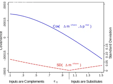
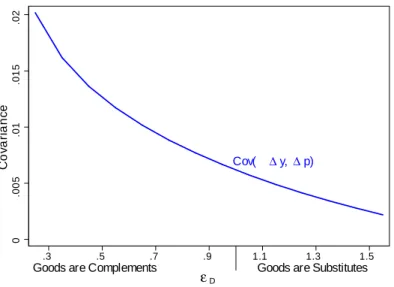
The purpose of this section is to provide some intuition as to how the model’s parameters are identi…ed. I do this in two ways. First, in Section 5.1, I consider an example econ-omy for which I can derive expressions for the covariances among industries prices, sales, and intermediate input cost shares. Second, in Section 5.2, I numerically relate "Q and
"D to various model-predicted moments (setting all other parameters to the Table-2 MLE
estimates). The aim of this second exercise is to illustrate how these two elasticities are identi…ed, and to show that the analytical results obtained in Section 5.1’s simple example are pertinent.
Section 5.1 demonstrates that if "Q < 1, then only industry-speci…c shocks can
account for the intermediate input cost shares that are both volatile and uncorrelated across industries (as documented in Section 3). The primary takeaway from Section 5.2 is that
"Q is estimated to be less than 1 mainly because of volatile intermediate input shares that
are positively correlated with the industries’own intermediate input prices. In combination, these two …ndings explain why industry-speci…c shocks are important.
5.1
A Simple Example
33In this section, I study a simple economy for which analytic expressions are available. The goal of this exercise is to explain why industry-speci…c shocks are more prominent
when "Q is freely estimated. To summarize the results of this exercise, when "Q = 1 only
measurement error can possibly generate any variation in the observed intermediate input cost shares. On the other hand, when "Q is less than 1, industry I’s intermediate input
cost shares also co-vary with its own industry-speci…c labor-augmenting productivity and 33This subsection is related to the technical appendix ofCarvalho and Gabaix (2013). The main di¤erences
are that Carvalho and Gabaix impose that "Q = 1 and also allow for some adjustment costs to aggregate
the aggregate factor-neutral productivity. When the aggregate factor-neutral productivity term is large, industries’intermediate input cost shares co-move. Thus, to …t the volatile, uncorrelated intermediate input cost shares, the MLE procedure assigns higher values to
B;Ind when"Q is freely estimated.
Compared to the benchmark model given in Section2, I make a number of simplifying assumptions. I assume that a) all goods depreciate fully each period; b) there is no physical capital in production; c) the exogeneous productivity and preference processes have zero persistence; d) each industry has identical production functions; e) the consumer’s preference weight is the same for each of theN goods; f) the input-output matrix has N1 in each entry; and g) "M = 0. For the reader’s convenience, I re-write the utility function and each
industry’s sectoral production function, incorporating these assumptions. Via assumptions (a) through (c), the equilibrium allocation can be solved period by period. For this reason, I omit time subscripts in this section.
The output of industry J equals:
QJ =AJ AAgg
0
@(1 )
1
"Q (B
J BAgg LJ)
"Q 1
"Q +
1
"Q 1
N minI MI!J
"Q 1
"Q 1 A
"Q
"Q 1
. (17)
Output is produced using labor LJ and intermediate inputsMI!J purchased from other
sectors. Note that the restriction of"M = 0is already incorporated in Equation17. Finally,
to emphasize, each sector’s production function is distinguished only by the industry-speci…c components of the two productivity terms. The cost share parameters ( J and M
IJ), which
were previously allowed to di¤er by industry, are now the same for each industry.
The representative consumer has preferences over leisure and the N consumption goods, parameterized by the following utility function:
U = DAgg N
X
J=1
DJ
N !
log 2 4
N
X
J=1
DJ
N 1
"D (CJ)
"D 1
"D
! "D
"D 13
5 "LS
"LS + 1 N
X
J=1
LJ
!"LS+1
"LS
. (18) As before, "D and"LS parameterize, respectively, the elasticity of substitution across the
consumption goods and the elasticity of labor supply. For future reference, de…ne the ideal price index of the consumption-good bundle as:
P
" N X
J=1
DJ
PN
I=1DI
(PJ)1 "D
# 1
1 "D