COMPRESSIVE SENSING BY RANDOM CONVOLUTION
JUSTIN ROMBERG∗
Abstract. This paper outlines a new framework for compressive sensing: convolution with a random waveform followed by random time domain subsampling. We show that sensing by random convolution is a universally efficient data acquisition strategy in that ann-dimensional signal which isSsparse in any fixed representation can be recovered fromm&Slognmeasurements. We discuss two imaging scenarios — radar and Fourier optics — where convolution with a random pulse allows us to seemingly super-resolve fine-scale features, allowing us to recover high-resolution signals from low-resolution measurements.
1. Introduction. The new field of compressive sensing (CS) has given us a fresh look at data acquisition, one of the fundamental tasks in signal processing. The message of this theory can be summarized succinctly [7, 8, 10, 15, 32]: the number of measurements we need to reconstruct a signal depends on its sparsity rather than its bandwidth. These measurements, however, are different than the samples that traditional analog-to-digital converters take. Instead of simple point evaluations, we model the acquisition of a signal x0 as a series of inner products against different
waveformsφ1, . . . , φm:
yk =hφk, x0i, k= 1, . . . , m. (1.1)
Recoveringx0from theyk is then a linear inverse problem. If we assume thatx0
and theφk are members of somen-dimensional space (the space ofn-pixel images, for
example), (1.1) becomes a system ofm×nlinear equations,y= Φx0. In general, we will need more measurements than unknowns,m≥n, to recoverx0fromy. But if the signal of interest x0 is sparse in a known basis, and theφk are chosen appropriately,
then results from CS have shown us that recovering x0 is possible even when there
are far fewer measurements than unknowns,mn.
The notion of sparsity is critical to compressive sensing — it is the essential measure of signal complexity, and plays roughly the same role in CS that bandwidth plays in the classical Shannon-Nyquist theory. When we say a signal is sparse it always in the context of an orthogonal signal representation. With Ψ as an n×n orthogonal representation matrix (the columns of Ψ are the basis vectors), we say x0 is S-sparse in Ψ if we can decompose x0 as x0 = Ψα0, whereα0 has at most S
non-zero components. In most applications, our signals of interest are not perfectly sparse; a more appropriate model is that they can be accurately approximated using a small number of terms. That is, there is a transform vectorα0,S with onlyS terms
such that kα0,S−α0k2 is small. This will be true if the transform coefficients decay like a power law — such signals are calledcompressible.
Sparsity is what makes it possible to recover a signal from undersampled data. Several methods for recovering sparsex0from a limited number of measurements have
been proposed [12,16,29]. Here we will focus on recovery via`1 minimization. Given
the measurementsy= Φx0, we solve the convex optimization program
min
α kαk`1 subject to ΦΨα=y. (1.2)
∗ School of Electrical and Computer Engineering, Georgia Tech, Atlanta, Georgia.
Email:[email protected]. This work was supported by DARPA’s Analog-to-Information pro-gram.
In words, the above searches for the set of transform coefficients α such that the measurements of the corresponding signal Ψα agree with y. The `1 norm is being
used to gauge the sparsity of candidate signals.
The number of measurements (rows in Φ) we need to take for (1.2) to succeed depends on the nature of the waveforms φk. To date, results in CS fall into one of
two types of measurement scenarios. Randomness plays a major role in each of them. 1. Random waveforms. In this scenario, the shape of the measurement wave-forms is random. The ensemble Φ is generated by drawing each element independently from a subgaussian [6, 10, 15, 24] distribution. The canonical examples are generating each entry Φi,j of the measurement ensemble as
in-dependent Gaussian random variables with zero mean and unit variance, or as independent Bernoulli±1 random variables.
The essential result is that ifx0isS-sparse in any Ψ and we make1
m &S·logn (1.3)
random waveform measurements, solving (1.2) will recoverx0 exactly.
2. Random sampling from an incoherent orthobasis. In this scenario, we select the measurement waveformsφkfrom rows of an orthogonal matrix Φ0 [7]. By
convention, we normalize the rows to have energykφkk22=n, making them the same size (at least on average) as in the random waveform case above. Them rows of Φ0 are selected uniformly at random from among all subsets
of rows of sizem. The principal example of this type of sensing is observing randomly selected entries of a spectrally sparse signal [8]. In this case, the φk are elements of the standard basis (and Φ0=nI), and the representation
Ψ is a discrete Fourier matrix.
When we randomly sample from a fixed orthosystem Φ0, the number of
sam-ples required to reconstructx0 depends on the relationship between Φ0 and
Ψ. One way to quantify this relationship is by using themutual coherence: µ(Φ0,Ψ) = max
φk∈Rows(Φ0)
ψj∈Columns(Ψ)
|hφk, ψji|. (1.4) Whenµ= 1, Φ0 and Ψ are as different as possible; each element of Ψ is flat
in the Φ0 domain. Ifx
0isS sparse in the Ψ domain, and we take
m & µ2·S·logn (1.5)
measurements, then (1.2) will succeed in recovering x0 exactly. Notice that
to have the same result (1.3) as the random waveform case,µwill have to be on the order of 1; we call such Φ0 and Ψincoherent.
There are three criteria which we can use to compare strategies for compressive sampling.
Universality. A measurement strategy is universal if it is agnostic towards the
choice of signal representation. This is the case when sensing with random waveforms. When Φ is a Gaussian ensemble this is clear, as it will remain Gaussian under any orthogonal transform Ψ. It is less clear but still true [6] 1Here and below we will use the notationX &Y to mean that there exists a known constant
C such that X ≥CY˙. For random waveforms, we actually have the the more refined bound of
that the strategy remains universal when the entries of Φ are independent and subgaussian.
Random sampling from a fixed system Φ0is definitely not universal, asµ(Φ0,Ψ)
cannot be on the order of 1 for every Ψ. We cannot, for example, sample in a basis which is very similar to Ψ (µ≈√n) and expect to see much of the signal.
Numerical structure. Algorithms for recovering the signal will invariably
in-volve repeated applications of ΦΨ and the adjoint Ψ∗Φ∗. Having an efficient
method for computing these applications is thus of primary importance. In general, applying anm×nmatrix to ann-vector requiresO(mn) operations; far too many ifnandm are only moderately large (in the millions, say). It is often the case that a Ψ which sparsifies the signals of interest comes equipped with a fast transform (the wavelet transform for piecewise smooth signals, for example, or the fast Fourier transform for signals which are spec-trally sparse). We will ask the same of our measurement system Φ.
The complete lack of structure in measurement ensembles consisting of ran-dom waveforms makes a fast algorithm for applying Φ out of the question. There are, however, a few examples of orthobases which are incoherent with sparsity bases of interest and can be applied efficiently. Fourier systems are perfectly incoherent with the identity basis (for signals which are sparse in time), and noiselets [13] are incoherent with wavelet representations and enjoy a fast transform with the same complexity as the fast Fourier transform.
Physically realizable. In the end, we have to be able to build sensors which
take the linear measurements in (1.1). There are architectures for CS where we have complete control over the types of measurements we make; a well-known example of this is the “single pixel camera” of [17]. However, it is often the case that we are exploiting a physical principle to make indirect observations of an object of interest. There may be opportunities for injecting randomness into the acquisition process, but the end result will not be taking inner products against independent waveforms.
In this paper, we introduce a framework for compressive sensing which meets all three of these criteria. The measurement process consists of convolving the signal of interest with a random pulse and then randomly subsampling. This procedure is random enough to be universally incoherent with any fixed representation system, but structured enough to allow fast computations (via the FFT). Convolution with a pulse of our choosing is also a physically relevant sensing architecture. In Section 2 we discuss two applications in particular: radar imaging and coherent imaging using Fourier optics.
1.1. Random Convolution. Our measurement process has two steps. We
cir-cularly convolve the signal x0 ∈ Rn with a “pulse” h∈ Rn, then subsample. The pulse is random, global, and broadband in that its energy is distributed uniformly across the discrete spectrum.
In terms of linear algebra, we can write the convolution ofx0andhasHx, where
H=n−1/2F∗ΣF,
withF as the discrete Fourier matrix
and Σ as a diagonal matrix whose non-zero entries are the Fourier transform of h. We generatehat random by taking
Σ =
σ1 0 · · ·
0 σ2 · · ·
... ...
σn
,
a diagonal matrix whose entries are unit magnitude complex numbers with random phases. We generate theσω as follows2:
ω= 1 : σ1∼ ±1 with equal probability,
2≤ω < n/2 + 1 : σω=ejθω, where θ
ω∼Uniform([0,2π]),
ω=n/2 + 1 : σn/2+1∼ ±1 with equal probability
n/2 + 2≤ω≤n : σω=σn−ω+2∗ , the conjugate of σn−ω+2.
The action ofH on a signalxcan be broken down into a discrete Fourier transform, followed by arandomization of the phase(with constraints that keep the entries ofH real), followed by an inverse discrete Fourier transform.
The construction ensures thatH will be orthogonal, H∗H =n−1F∗Σ∗F F∗ΣF =nI,
sinceF F∗ =F∗F =nI and Σ∗Σ =I. Thus we can interpret convolution withhas
a transformation into a random orthobasis.
1.2. Subsampling. Once we have convolved x0 with the random pulse, we
“compress” the measurements by subsampling. We consider two different methods for doing this. In the first, we simply observe entries of Hx0 at a small number of
randomly chosen locations. In the second, we breakHx0into blocks, and summarize
each block with a single randomly modulated sum.
1.2.1. Sampling at random locations. In this scheme, we simply keep some
of the entries of Hx0 and throw the rest away. If we think of Hx0 as a set of
Nyquist samples for a bandlimited function, this scheme can be realized by with an analog-to-digital converter (ADC) that takes non-uniformly spaced samples at an average rate which is appreciably slower than Nyquist. Convolving with the pulseh combines a little bit of information about all the samples in x0 into each sample of Hx0, information which we can untangle using (1.2).
There are two mathematical models for sampling at random locations, and they are more or less equivalent. The first is to set a sizem, and select a subset of locations Ω⊂ {1, . . . , n}uniformly at random from all mn
subsets of sizem. The second is to generate an iid sequence of Bernoulli random variablesι1, . . . , ιn, each of which takes
a value of 1 with probabilitym/n, and sample at locations t where ιt= 1. In this
case, the size of the sample set Ω will not be exactlym. Nevertheless, it can be shown (see [8] for details) that if we can establish successful recovery with probability 1−δ for the Bernoulli model, we will have recovery with probability 1−2δin the uniform model. Since the Bernoulli model is easier to analyze, we will use it throughout the rest of the paper.
In either case, the measurement matrix can be written as Φ =RΩH, where RΩ
is the restriction operator to the set Ω.
1.2.2. Randomly pre-modulated summation. An alternative to simply
throw-ing away most of the samples ofHx0 is to break them into blocks of size n/m, and
summarize each block with a single number. To keep things simple, we will assume that m evenly divides n. With Bk = {(k−1)n/m+ 1, . . . , kn/m}, k = 1, . . . , m
denoting the index set for blockk, we take a measurement by multiplying the entries of Hx0 in Bk by a sequence of random signs and summing. The corresponding row
of Φ is then
φk= rm
n
X
t∈Bk
tht, (1.6)
where ht is the tth row of H. The {p}np=1 are independent and take a values of
±1 with equal probability, and the factorp
m/nis a renormalization that makes the norms of theφk similar to the norm of theht. We can write the measurement matrix
as Φ =PΘH, where Θ is a diagonal matrix whose non-zero entries are the{p}, and P sums the result over each blockBk.
In hardware, randomly pre-modulated summation (RPMS) can be implemented by multiplying the incoming signal by a high-rate (Nyquist or above) chipping se-quence, effectively changing the polarity across short time intervals. This is followed by an integrator (to compute the analog of the sum in (1.6)) and an ADC taking equally spaced samples at a rate much smaller than Nyquist. This acquisition strat-egy is analyzed (without the convolution with h) in [33], where it is shown to be effective for capturing spectrally sparse signals. In Section 2.2, we will also see how RPMS can be used in certain imaging applications.
The recovery bounds we derive for random convolution followed by RPMS will essentially be the same (to within a single log factor) as in the random subsampling scheme. But RPMS has one important advantage: it “sees” more of the signal than random subsampling without any amplification. Suppose that the energy in Hx0 is
spread out more or less evenly across all locations — this is, after all, one of the purposes of the random convolution. If the energy (`2 norm squared) in the entire
signal is 1, then the energy in each sample will be about 1/n, and the energy in each block will be aboutn/m. If we simply takemsamples, the total energy in the measurements will be aroundm/n. If we take a random sum as in (1.6) (without the renormalization factor) over a blockBk of sizen/m, the expected squared magnitude
of this single measurement will be the same as the energy ofHx0inBk, and the total
energy of all the measurements will be (in expectation) the same as the energy in Hx0. So RPMS is an architecture for subsampling which will on average retain all of
the signal energy.
It is important to understand that the summation in (1.6) must be randomly modulated. Imagine if we were to leave out the {t} and simply sum Hx0 over each Bk. This would be equivalent to putting Hx0 through a boxcar filter then
subsampling uniformly. Since boxcar filteringHx0is also a convolution, it commutes
with H, so this strategy would be equivalent to first convolving x0 with the boxcar
filter, then convolving withh, then subsampling uniformly. But now it is clear how the convolution with the boxcar hurts us: it filters out the high frequency information inx0, which cannot be recovered no matter what we do next.
We will see that while coherent summation will destroy a sizable fraction of this signal, randomly pre-modulated summation does not. This fact will be especially important in the imaging architecture discussed in Section 2.2, where measurements are taken by averaging over large pixels.
1.3. Main Results. Both random subsampling [8] and RPMS [33] have been
shown to be effective for compressive sampling of spectrally sparse signals. In this paper, we show that preceding either by a random convolution results in auniversal compressive sampling strategy.
Our first theoretical result shows that if we generate a random pulse as in Sec-tion 1.1 and a random sampling pattern as in SecSec-tion 1.2.1, then with high probability we will be able to sense the vast majority of signals supported on a fixed set in the Ψ domain.
Theorem 1.1. Let Ψ be an arbitrary orthonormal signal representation. Fix a support set Γ of size |Γ| =S in the Ψ domain, and choose a sign sequence z on Γ uniformly at random. Let α0 be a set ofΨ domain coefficients supported on Γ with signsz, and takex0= Ψα0 as the signal to be acquired. Create a random convolution matrixH as described in Section 1.1, and choose a set of sample locations Ωof size |Ω|=muniformly at random with
m≥C0·S·log(n/δ) (1.7)
and also m≥ C1log3(n/δ), whereC0 andC1 are known constants. Set Φ = RΩH. Then given the set of samples on Ω of the convolution Hx0, y = Φx0, the program (1.2)will recoverα0 (and hencex0) exactly with probability exceeding 1−δ.
Roughly speaking, Theorem 1.1 works because if we generate a convolution matrix H at random, with high probability it will be incoherent with any fixed orthonormal matrix Ψ. Actually using the coherence defined in (1.4) directly would give a slightly weaker bound (log2(n/δ) instead of log(n/δ) in (1.7)); our results will rely on a more
refined notion of coherence which is outline in Section 3.1.
Our second result shows that we can achieve similar acquisition efficiency using the RPMS.
Theorem 1.2. Let Ψ,Γ, α0, x0, and H be as in Theorem 1.1. Create a random
pre-modulated summation matrix PΘ as described in Section 1.2.1 that outputs a number of samples mwith
m≥C0·S·log2(n/δ) (1.8)
and also m≥C1log4(n/δ), where C0 andC1 are known constants. Set Φ =PΘH. Then given the measurementsy= Φx0, the program (1.2)will recoverα0 (and hence x0) exactly with probability exceeding1−δ. The form of the bound (1.8) is the same
as using RPMS (again, without the random convolution in front) to sense spectrally sparse signals.
At first, it may seem counterintuitive that convolving with a random pulse and subsampling would work equally well with any sparsity basis. After all, an application ofH =n−1/2F∗ΣFwill not change the magnitude of the Fourier transform, so signals
which are concentrated in frequency will remain concentrated and signals which are spread out will stay spread out. For compressive sampling to work, we need Hx0
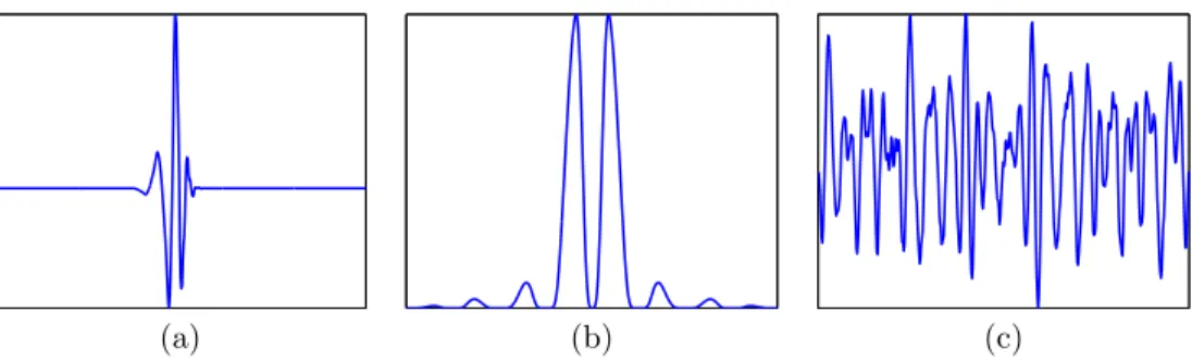
to be “spread out” in the time domain. We already know that signals which are concentrated on a small set in the Fourier domain will be spread out in time [8]. The randomness of Σ will make it highly probable that a signal which is concentrated in time will not remain so after H is applied. Time localization requires very delicate relationships between the phases of the Fourier coefficients, when we blast the phases by applying Σ, these relationships will no longer exist. A simple example of this phenomena is shown in Figure 1.1.
(a) (b) (c)
Fig. 1.1.(a) A signalx0 consisting of a single Daubechies-8 wavelet. Taking samples at random locations of this wavelet will not be an effective acquisition strategy, as very few will be located in its support. (b) Magnitude of the Fourier transformF x0. (c) Inverse Fourier transform after the phase has been randomized. Although the magnitude of the Fourier transform is the same as in (b), the signal is now evenly spread out in time.
1.4. Relationship to previous research. In [1], Ailon and Chazelle propose
the idea of a randomized Fourier transform followed by a random projection as a “fast Johnson-Lindenstrauss transform” (FJLT). The transform is decomposed as QFΣ, where Qis a sparse matrix with non-zero entries whose locations and values are chosen at random locations. They show that this matrix QFΣ behaves like a random waveform matrix in that with extremely high probability, it will not change the norm of an arbitrary vector too much. However, this construction requires that the number of non-zero entries in each row ofQis commensurate with the number of rowsmofQ. Although ideal for dimensionality reduction of small point sets, this type of subsampling does not translate well to compressive sampling, as it would require us to randomly combine on the order ofmsamples ofHx0from arbitrary locations to
form a single measurement — takingmmeasurements would require on the order of m2 samples. We show here that more structured projections, consisting either of one
randomly chosen sample per row or a random combination of consecutive samples, are adequate for CS. This is in spite of the fact that our construction results in much weaker concentration than the FJLT.
The idea that the sampling rate for a sparse (“spikey”) signal can be significantly reduced by first convolving with a kernel that spreads it out is one of the central ideas of sampling signal with finite rates of innovation [23,35]. Here, we show that a random kernel works for any kind sparsity, and we use an entirely different reconstruction framework.
In [34], numerical results are presented that demonstrate recovery of sparse signals (using orthogonal matching pursuit instead of`1 minimization) from a small number
of samples of the output of a finite length “random filter”. In this paper, we approach things from a more theoretical perspective, deriving bounds on the number of samples need to guarantee sparse reconstruction.
In [4], random convolution is explored in a slightly different context than in this paper. Here, the sensing matrix Φ consists of random selected rows (or modulated sums) of a Toeplitz matrix; in [4], the sensing matrix is itself Toeplitz, corresponding to convolution followed by a small number of consecutive samples. This difference in structure will allow us to derive stronger bounds: (1.7) guarantees recovery from Slognmeasurements, while the bound in [4] requires S2logn.
2. Applications. The fact that random convolution is universal and allows fast
section, we briefly discuss two imaging scenarios (in a somewhat rarified stetting) in which convolution with a random pulse can be implemented naturally.
We begin by noting that while Theorems 1.1 and 1.2 above deal explicitly with circular convolution, what is typically implemented is linear convolution. One simple way to translate our results to linear convolution would be to repeat the pulseh; then the samples in the midsection of the linear convolution would be the same as samples from the circular convolution.
2.1. Radar imaging. Reconstruction from samples of a signal convolved with
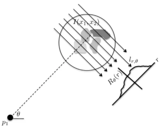
a known pulse is fundamental in radar imaging. Figure 2.1 illustrates how a scene is measured in spotlight synthetic aperture radar (SAR) imaging (see [25] for a more in-depth discussion). The radar, located at pointp1, focusses its antenna on the region
of interest with reflectivity functionI(x1, x2) whose center is at orientationθrelative
top1, and sends out a pulseh(t). If the radar is far enough away from the region of
interest, this pulse will arrive at every point along one of the parallel lines at a certain rangerat approximately the same time. The net reflectivity from this range is then the integralRθ(r) ofI(x1, x2) over the line atlr,θ,
Rθ(r) = Z
lr,θ
I(x1, x2)dx1dx2,
and the return signaly(t) is thus the pulse convolved withRθ
y(t) =h∗Rθ,
where it is understood that we can convertRθ from a function of range to a function
of time by dividing by the speed at which the pulse travels.
The question, then, is how many samples of y(t) are needed to reconstruct the range profileRθ. A classical reconstruction will require a number of samples
propor-tional to the bandwith of the pulseh; in fact, the sampling rate of the analog-to-digital converter is one of the limiting factors in the performance of modern-day radar sys-tems [26]. The results outlined in Section 1.3 suggest that if we have an appropriate representation for the range profiles and we use a broadband random pulse, then the number of samples needed to reconstruct anRθ(r) using (1.2) scales linearly with the
complexityof these range profiles, and onlylogarithmicallywith the bandwidth of h. We can gain the benefits of a high-bandwidth pulse without paying the cost of an ADC operating at a comparably fast rate.
A preliminary investigation of using ideas from compressive sensing in radar imag-ing can be found in [5]. There has also been some recent work on implementimag-ing low-cost radars which use random waveforms [2, 3] and traditional image reconstruc-tion techniques. Also, in [19], it is shown that compressive sensing can be used to super-resolve point targets when the radar sends out an incoherent pulse.
2.2. Fourier optics. Convolution with a pulse of our choosing can also be
im-plemented optically. Figure 2.2 sketches a possible compressive sensing imaging archi-tecture. The object is illuminated by a coherent light source; one might think of the object of interest as a pattern on a transparency, and the image we want to acquire as the light field exiting this transparency. The first lens takes an optical Fourier transform of the image, the phase of the Fourier transform is then manipulated using a spatial light modulator. The next lens inverts the Fourier transform, and then a second spatial light modulator and a low-resolution detector array with “big pixels” affect the RPMS subsampling scheme. In this particular situation, we will assume
lr,θ
I(x1, x2)
Rθ(r
)
r
θ p1
Fig. 2.1.Geometry for the “spotlight SAR” imaging problem. The return signal from a pulseh(t)emitted from pointp1 will be the range profileRθ(r) (collection of line integrals at an angleθ) convolved withh.
that our detectors can observe both the magnitude and the phase of the final light field (modern heterodyne detectors have this capability).
Without the spatial light modulators, the resolution of this system scales with the size of the detector array. The big-pixel detectors simply average the light field over a relatively large area, and the result is a coarsely pixellated image. Adding the spatial light modulators allows us to effectively super-resolve this coarse image. With the SLMs in place, the detector is taking incoherent measurements in the spirit of Theorem 1.2 above. The resolution (for sparse images and using the reconstruction (1.2)) is now determined by the SLMs: the finer the grid over which we can effectively manipulate the phases, the more effective pixels we will be able to reconstruct.
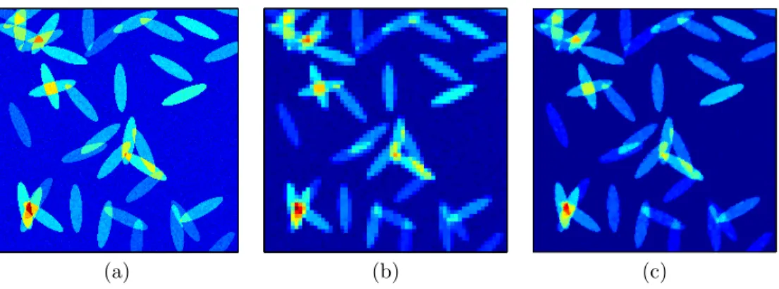
Figure 2.3 illustrates the potential of this architecture with a simple numerical experiment3. A 256×256 synthetic image, was created by placing 40 ellipses —
with randomly chosen orientations, positions, and intensities — and adding a modest amount of noise. Measuring this image with a 64×64 “low resolution” detector array produces the image in Fig. 2.3(b), where we have simply averaged the image in part (a) over 4×4 blocks. Figure 2.3(c) is the result when the low resolution measurements are augmented with measurements from the architecture in Figure 2.2. With x0 as
the underlying image, we measurey= Φx0, where
Φ =PΘPH.
From these measurements, the image is recovered using total variation minimization, a variant of`1 minimization that tends to give better results on the types of images
being considered here. Giveny, we solve min
x TV(x) subject to kΦx−yk2≤,
where is a relaxation parameter set at a level commensurate with the noise. The result is shown in Figure 2.3(c). As we can see, the incoherent measurements have 3Matlab code that reproduces this experiment can be downloaded at users.ece.gatech.edu/∼justin/randomconv/ .
!"#$%&
x0
'%()&
F *+,&Σ '%()&F∗ *+,&Θ -%.%/.01#2&P
y=PΘHx0
34,*& 1#(-0"&/0(50'670(&H
Fig. 2.2.Fourier optics imaging architecture implementing random convolution followed by RPMS. The computationy = PΘHx0 is done entirely in analog; the lenses move the image to the Fourier domain and back, and spatial light modulators (SLMs) in the Fourier and image planes randomly change the phase.
(a) (b) (c)
Fig. 2.3. Fourier optics imaging experiment. (a) The “high-resolution” image we wish to acquire. (b) The high-resolution image pixellated by averaging over 4×4 blocks. (c) The image restored from the pixellated version in (b), plus a set of incoherent measurements taken using the architecture from Figure 2.2. The incoherent measurements allow us to effectively super-resolve the image in (b).
allowed us to super-resolve the image; the boundaries of the ellipses are far clearer than in part (b).
The architecture is suitable for imaging with incoherent illumination as well, but there is a twist. Instead of convolution with the random pulseh(the inverse Fourier transform of the mask Σ), the lens-SLM-lens system convolves with |h|2. While |h|2 is still random, and so the spirit of the device remains the same, convolution with|h|2 is no longer a unitary operation, and thus falls slightly outside of the mathematical framework we develop in this paper.
3. Theory.
3.1. Coherence bounds. First, we will establish a simple bound on the
co-herence parameter between a random convolution system and a given representation system.
Lemma 3.1. Let Ψ be an arbitrary fixed orthogonal matrix, and create H at random as above with H = n−1/2F∗ΣF. Choose 0 < δ < 1. Then with probability exceeding1−δ, the coherenceµ(H,Ψ) will obey
Proof. The proof is a simple application of Hoeffding’s inequality (see Appendix A). Ifhtis thetth row ofH (measurement vector) andψsis thesth column of Ψ
(repre-sentation vector), then
hht, ψsi=
n X
ω=1
ej2π(t−1)(ω−1)/nσ ωψˆs(ω),
where ˆψsis the normalized discrete Fourier transformn−1/2F ψs. Sincehtandψsare
real-valued and theσω are conjugate symmetric, we can rewrite this sum as
hht, ψsi=σ1ψˆs(1) + (−1)t−1σn/2+1ψˆs(n/2 + 1) + 2
n/2 X
ω=2
RehF∗
t,ωσωψˆs(ω) i
, (3.2) where we have assumed without loss of generality thatnis even; it will be obvious how to extend to the case wherenis odd. Now each of theσωin the sum above are
inde-pendent. Because theσωare uniformly distributed on the unit circle, Re[Ft,ω∗ σωψˆs(ω)]
has a distribution identical toω|ψˆs|cos(ˆθ(ω)), where ˆθ(ω) is the phase of ˆψs(ω)Ft,ω∗
and{ω} is an independent random sign sequence. Thus,
n/2+1 X
ω=1
ωaω, with aω=
ˆ
ψs(1), ω= 1
2|ψˆs|cos(ˆθ(ω)), 2≤ω≤n/2 ˆ
ψs(n/2 + 1), ω=n/2 + 1
has a distribution identical tohht, ψsi. Since
n/2+1 X
ω=1
a2
ω≤2kψsk22= 2,
applying the bound (A.1) gives us P
n/2+1 X
ω=1
a2 ω
> λ
≤2e−λ 2/4
. Takingλ= 2p
log(2n2/δ) and applying the union bound over alln2 choices of (t, s)
establishes the lemma.
Appling Lemma 3.1 directly to the recovery result (1.5) guarantees recovery from m&S·log2n
randomly chosen samples, a log factor off of (1.7). We are able to get rid of this extra log factor by using a more subtle property of the random measurement ensembleH. Fix a subset Γ of the Ψ domain of size |Γ|=S, and let ΨΓ be then×S matrix consisting of the columns of Ψ indexed by Γ. In place of the coherence, our quantity of interest will be
ν :=ν(Γ) = max
k=1,...,nkr kk
with therk as rows in the matrixHΨ
Γ; we will callν(Γ) the cumulative coherence
Γ (this quantity was also used in [32]). We will show below that we can bound the number of measurements needed to recover (with high probability) a signal on Γ by
m&ν2·logn.
Since we always have the boundν ≤µ√S, the result (1.5) is still in effect. However, Lemma 3.2 below will show that in the case where U = HΨ with H as a random convolution matrix, we can do better, achievingν .√S.
Lemma 3.2. Fix an orthobasisΨand a subset of theΨ-domainΓ ={γ1, . . . , γS}
of size |Γ|=S Generate a random convolution matrix H at random as described in Section 1.1 above, and letrk, k= 1, . . . , nbe the rows ofHΨΓ. Then with probability exceeding1−δ
ν(Γ) = max
k=1,...,nkr kk
2≤
√
8S, (3.4)
forS≥16 log(2n/δ).
Proof. of Lemma 3.2. We can write rk as the following sum of random vectors
inCS:
rk =Xn ω=1
Fk,ωσ∗ωgω,
wheregω∈CS is a column of ˆΨ∗Γ:
gω=
ˆ ψγ1(ω)∗
ˆ ψγ2(ω)∗
. . . ˆ ψγS(ω)∗
.
By conjugate symmetry, we can rewrite this as a sum of vectors inRS, rk =σ
1g1+σn/2+1(−1)k−1gn/2+1+ 2 n/2 X
ω=2
Re [Fk,ωσ∗ωgω]
(note thatg1andgn/2+1will be real-valued). Because theσωare uniformly distributed
over the unit circle, the random vector Re[Fk,ωσω∗gω] has a distribution identical to
ωRe[Fk,ωσ∗ωgω], whereω is an independent Rademacher random variable. We set
Y =
n/2+1 X
ω=1
ωvω, where vω=
g1 ω= 1
2 Re [Fk,ωσ∗ωgω] 2≤ω≤n/2
gn/2+1 ω=n/2 + 1
.
and will show that with high probabilitykYk2will be within a fixed constant of√S. We can bound the mean ofkYk2as follows:
E[kYk2]2 ≤ E[kYk22] =
n/2+1 X
ω=1
kvωk22 ≤ 2
n X
ω=1
where the last inequality come from the facts that kvωk22 ≤ 4kgωk22 and kgωk22 = kgn−ω+2k22forω= 2, . . . , n/2.
To show thatkYkis concentrated about its mean, we use a concentration inequal-ity on the norm of a sum of random vector, specifically (A.3) which is detailed in the Appendix.
To apply this bound first note that for any vectorξ∈Rs |hξ,Re[Fk,ωσω∗gω]i|2 ≤ |hξ, gωi|2. Thus
sup
kξk2≤1 n/2+1
X
ω=1
|hξ, vωi|2≤2 sup
kξk2≤1 n X
ω=1
|hξ, gωi|2 = 2 sup
kξk2≤1ξ TΨT
ΓΨΓξ
= 2. We now apply (A.3) to get
PkYk2≥√2S+λ ≤ P (kYk2≥EkYk2+λ) ≤ 2e−λ2/32 and so for anyC >√2,
Pkrkk2≥C√S= PkYk2≥C√S≤2e−(C−√2)2S/32≤δ/n
whenS ≥32(C−√2)−2log(2n/δ). TakingC= 2√2 and applying the union bound overk= 1, . . . , nestablishes the lemma.
3.2. Sparse Recovery. The following two results extends the main results of [7]
and [33] to take advantage of our more refined bound on the norm coherence M. Theorems 3.3 and 3.4 are stated for general measurement systems U with U∗U =
nI, as they may be of independent interest. Theorems 1.1 and 1.2 are then simple applications withU =HΨ and the bound (3.4) onν(Γ).
Here and below we will useUΓ for then×S matrix consisting of the columns of
U indexed by the set Γ.
Theorem 3.3. LetU be an×n orthogonal matrix with U∗U =nI with mutual coherenceµ. Fix a subsetΓ, let rk be the rows ofUΓ, and setν := maxk=1,...,nkrkk2. Choose a subsetΩof the measurement domain of size|Ω|=m and a sign sequencez onΓ uniformly at random. SetΦ =RΩU, the matrix constructed from the rows of U indexed byΩ. Suppose that
m≥C0·ν2·log(n/δ),
and also m ≥ C00 ·µ2log2(n/δ) where C0 and C00 are known constants. Then with probability exceeding 1−O(δ), every vector α0 supported on Γ with sign sequence z can be recovered fromy= Φα0 by solving (1.2).
Theorem 3.4. Let U, µ,Γ, ν, z be as in Theorem 3.3. Create an RPMS matrix PΘas in Section 1.2.2, and setΦ =PΘU. Suppose that
and also m ≥ C10 ·µ2log3(n/δ) where C1 and C10 are known constants. Then with probability exceeding 1−O(δ), every vector α0 supported on Γ with sign sequence z can be recovered fromy= Φα0 by solving (1.2).
The proofs of Theorems 3.3 and 3.4 follow the same general outline put forth in [7], with with one important modification (Lemmas 3.5 and 3.6 below). As detailed in [8,18,31], sufficient conditions for the successful recovery of a vectorα0supported
on Γ with sign sequencez are that ΦΓ has full rank, where ΦΓ is them×S matrix
consisting of the columns of Φ indexed by Γ, and that
|π(γ)|=|h(Φ∗ΓΦΓ)−1Φ∗Γϕγ, zi|<1 for all γ∈Γc, (3.5) whereϕγ is the column of Φ at indexγ.
There are three essential steps in establishing (3.5):
1. Show that with probability exceeding 1−δ, the random matrix Φ∗ΓΦΓ will have a bounded inverse:
k(Φ∗ΓΦΓ)−1k ≤2/m, (3.6) wherek·kis the standard operator norm. This has already been done for us in both the random subsampling and the RPMS cases. For random subsampling, it is essentially shown in [7, Th.1.2] that this is true when
m ≥ ν2·max(C1logS, C2log(3/δ)),
for given constantsC1, C2. For RPMS, a straightforward generalization of [33,
Th. 7] establishes (3.6) for
m ≥ C3·ν2·log2(S/δ). (3.7) 2. Establish, again with probability exceeding 1−O(δ), that the norm of Φ∗Γϕγ is on the order ofν√m. This is accomplished in Lemmas 3.5 and 3.6 below. Combined with step 2, this means that the norm of (Φ∗
ΓΦΓ)−1ϕγ is on the
order ofν/√m.
3. Given that k(Φ∗ΓΦΓ)−1ϕγk2 ∼ ν/√m, show that |π(γ)| < 1 for all γ ∈ Γc with probability exceeding 1−O(δ). Taking z as a random sign sequence, this is a straightforward application of the Hoeffding inequality.
3.3. Proof of Theorem 3.3. As step 1 is already established, we start with
step 2. We will assume without loss of generality thatm1/2≤ν/µ, as the probability
of success monotonically increases as m increases. The following lemma shows that kΦ∗Γϕγk2∼ν/√mfor eachγ∈Γc.
Lemma 3.5. LetΦ, µ,Γ, ν, andmbe as in Theorem 3.3. Fixγ∈Γc, and consider the random vector vγ = Φ∗Γϕγ =UΓ∗R∗Ωϕγ. Assume that √m≤ν2/µ. Then for any a≤2m1/4µ−1/2,
PkΦ∗Γϕγk2≥ν√m+aµ1/2m1/4ν≤3e−Ca2, whereC is a known constant.
Proof. We show that the mean Ekvγk2 is less than ν√m, and then apply the Talagrand concentration inequality to show thatkvγk2is concentrated about its mean.
Using the Bernoulli sampling model, Φ∗
Γϕγcan be written as a sum of independent
random variables, Φ∗
Γϕγ = n X
k=1
ιkUk,γrk = n X
k=1
(ιk−m/n)Uk,γrk,
where rk is the kth row of U
Γ = HΨΓ, and the second equality follows from the
orthogonality of the columns ofUΓ. To bound the mean, we use
E[kΦ∗Γϕγk2]2≤E[|hΦ∗Γϕγ,Φ∗Γϕγi|2] =
n X
k1,k2=1
E[(ιk1−m/n)(ιk2−m/n)]Uk1,γUk2,γhrk1, rk2i
= n X k=1 m n 1−m
n
U2 k,γkrkk22
≤ mν2 n n X k=1 U2 k,γ
=mν2.
We will apply Talagrand (see (A.4) in the Appendix) usingYk = (Ik−m/n)Uk,γrk.
Note that for allf ∈RS withkfk2≤1,
|hf, Yki| ≤ |Uk,γ| · |hf, rki| ≤µν, and so we can useB=µν. For ¯σ2, note that
E|hf, Yki|2= m n
1−m
n
· |Uk,γ|2· |hf, rki| and so
¯ σ2= sup
f n X
k=1
E|hf, Yki|2 =m
n
1−m
n
µ2Xn k=1
|hf, rki|2 ≤mµ2.
Plugging the bounds for EkΦ∗Γϕγk2,B, and ¯σ2 into (A.4), we have P kΦ∗Γϕγk2> ν√m+t
≤3 exp
− t Kµνlog
1 + mµ2+µνtµν2√ m
. Using our assumption that √m ≤ ν2/µ and the fact that log(1 +x) >2x/3 when 0≤x≤1, this becomes
P kΦ∗Γϕγk2> ν√m+t
≤3 exp
− t
2
3Kµ√mν2
for all 0≤t≤2ν√m. Thus
fora≤2m1/4µ−1/2, where C= 1/(3K).
To finish off the proof of the Theorem, letAbe the event that (3.6) holds; step 1 tells us that P(Ac)≤δ. LetBλ be the event that
max
γ∈Γck(Φ
∗
ΓΦΓ)−1vγk2≤λ.
By Lemma 3.5 and taking the union bound over allγ∈Γc, we have P(Bλc | A)≤3ne−Ca2.
By the Hoeffding inequality, Psup
γ∈Γc
|π(γ)|>1| Bλ,A
≤2ne−1/2λ2. Our final probability of success can then be bounded by
P
max
γ∈Γc|π(γ)|>1
≤P
max
γ∈Γc|π(γ)|>1| Bλ,A
+ P (Bλ|A) + P(A) ≤2ne−1/2λ2+ 3ne−Ca2+δ. (3.8) Choose λ = 2νm−1/2+ 2aµ1/2m−3/4ν. Then we can make the second term in
(3.8) less thanδby choosing a=C−1/2p
log(3n/δ); form≥16C−2µ2log2(3n/δ) we will havea≤(1/2)m1/4µ−1/2. This choice of aalso ensures thatλ≤3νm−1/2. For the first term in (3.8) to be less than δ, we need λ2 ≤(2 log(2n/δ))−1, which hold
when
m≥18·ν2·log(2n/δ).
3.4. Proof of Theorem 3.4. As before, we control the norm of Φ∗Γφγ (now
with Φ = PΘU), and then use Hoeffding to establish (3.5) with high probability. Lemma 3.6 says thatkΦ∗Γϕγk2∼√mν√lognwith high probability.
Lemma 3.6. Let Φ, µ,Γ, ν, andm be as in Theorem 3.4. Fix γ ∈Γc. Then for any δ >0
PkΦ∗Γφγk2> Cm1/2plog(n/δ)ν+ 4µplog(2n2/δ)= 2δ/n, whereC is a known constant.
Proof. To start, note that we can write Φ∗Γφγ as Φ∗
Γφγ =mn m X
k=1 X
p1,p2∈Bk
p1p2Up2,γrp1
=mn Xm k=1
X
p1,p2∈Bk
p16=p2
p1p2Up2,γrp1
since
m X
k=1 X
p∈Bk
by the orthogonality of the columns ofU. To decouple the sum above, we must first make it symmetric:
Φ∗
Γφγ= 2mn m X k=1 X p1,p2∈Bk p16=p2
p1p2(Up2,γrp1+Up1,γrp2).
Now, if we set Z= m 2n m X k=1 X p1,p2∈Bk p16=p2
p10p2(Up2,γrp1+Up1,γrp2) 2 , (3.9)
where the sequence{0i}is an independent sign sequence distributed the same as{i}, we have (see [14, Chapter 3])
P(kΦ∗Γφγk2> λ)< CDP(Z > λ/CD) (3.10) for some known constantCD, and so we can shift our attention to boundingZ.
We will bound the two parts of the random vector separately. Let vγ= mn
m X k=1 X p1,p2∈Bk p16=p2
p10p2Up2,γrp1.
We can rearrange this sum to get vγ = mn
m X k=1 X p∈Bk n/m−1 X q=1
p0(p+q)kU(p+q)k,γr
p (where (p+q)
k is addition moduloBk)
= m n n/m−1 X q=1 q m X k=1 X p∈Bk p q 0
(p+q)kU(p+q)k,γr
p
= mn
n/m−1 X q=1 q m X k=1 X p∈Bk 00
(p+q)kU(p+q)k,γr
p (where{00
i} is an iid sign sequence independent of{q})
= mn
n/m−1 X
q=1
qwq, where wq = m X k=1 X p∈Bk 00
(p+q)kU(p+q)k,γr
p.
We will show thatkwqk2can be controlled properly for each q, and then use the a concentration inequality to control the norm ofvγ. We start by bounding the mean
ofkwqk2:
(Ekwqk2)2≤Ekwqk22 = m X k=1 X p∈Bk U2
(p+q)k,γkr
pk2 2
≤ν2
n X
i=1
U2 i,γ
Using (A.3), we have that
P kwqk2>√n·ν+λ
≤ 2e−λ2/16σ2, where
σ2= sup kξk2≤1ξ
TV VTξ, with V := U
(1−q)k,γr1 U(2−q)k,γr2 · · · U(n−q)k,γrn
=U∗ ΓD,
andD is a diagonal matrix with theU·,γ along the diagonal. Since σ2 is the largest
(squared) singular value of V, and since kUΓ∗k = √n and kDk ≤ µ, we have that σ2≤nµ2. Thus
P kwqk2>√n·ν+λ
≤ 2e−λ2/16nµ2.
LetMλ be the event that all of thekwqk2 are close to their mean, specifically max
q=1,...,n/mkwqk2 ≤
√
n·ν+λ, and note that
P(Mcλ) ≤ 2nm−1e−λ2/nµ2. (3.11) Then
P(kvγk2> α)≤P(kvγk2> α|Mλ) + P(Mcλ). (3.12) Given that Mλ has occurred, we will now control kvγk2. Again, we start with the expectation
E[kvγk22| Mλ] = m2 n2
X
q1,q2
E[q1q2|Mλ] E[hwq1, wq2i|Mλ]
= mn22 X q1,q2
E[q1q2] E[hwq1, wq2i|Mλ]
= mn22X q
E[kwqk22|Mλ] ≤ m2
n2 X
q
(√nν+λ)2
= m n(
√
nν+λ)2.
Using Khintchine-Kahane ((A.2) in the Appendix), we have
Pkvγk2> C0m1/2n−1/2(n1/2ν+λ)plog(n/δ)| Mλ ≤ δ/n. (3.13) Choosingλ= 4n1/2µp
log(2n2/mδ), we fold (3.11) and (3.13) into (3.12) to get
Pkvγk2> C0m1/2plog(n/δ)ν+ 4µplog(2n2/mδ)≤2δ/n (3.14) By symmetry, we can replace kvγk2 with Z in (3.14), and arrive at the lemma by applying the decoupling result (3.10).
We finish up the proof of Theorem 3.4 by again applying the Hoeffding inequality. LetAbe the event that the spectral bound (3.6) holds; we know that P(Ac)≤δ for mas in (3.7). LetBbe the event that
max
γ∈Γc k(Φ
∗
ΓΦΓ)−1Φ∗Γϕ)γk2≤2Cm−1/2plog(n/δ)
ν+ 4µp
log(2n2/δ),
where the constantCis the same as that in Lemma 3.6; we have shown that P(Bc|A)≤ 2δ. By the Hoeffding inequality
P
sup
γ∈Γc
|π(γ)|>1| B,A
≤2nexp − m
8C2log(n/δ)(ν+ 4µp
log(2n2/mδ)) !
. (3.15) Whenν≥4µp
log(2n2/mδ), as will generally be the case, the left-hand side of (3.15)
will be less thanδwhen
m≥Const·ν2·log(n/δ). Whenν <4µp
log(2n2/mδ), the left-hand side of (3.15) will be less thanδwhen
m≥Const·µ2·log3(n/δ). The theorem then follows from a union bound withAandB.
4. Discussion. Theorems 1.1 and 1.2 tell us that we can recover a perfectly
S sparse signal from on the order ofSlogn, in the case of random subsampling, or Slog2n, in the case of random pre-modulated summation, noiseless measurements. If
we are willing to pay additional log factors, we can also guarantee that the recovery will be stable. In [27], it is shown that if Φ is generated by taking random rows from an orthobasis, then with high probability it will obey theuniform uncertainty principlewhen
m&µ2·S·log4n.
The connection between the uniform uncertainty principle and stable recovery via`1
minimization is made in [9–11]. Along with Lemma 3.1, we have stable recovery from a randomly subsampled convolution from
m&S·log5n
measurements. There is also a uniform uncertainty principle for an orthobasis which has been subsampled using randomly pre-modulated summation [30] with an addi-tional log factor; in this case, stable recovery would be possible from m&S·log6n measurements.
The results in this paper depend on the fact that different shifts of the pulse h are orthogonal to one another. But how critical is this condition? For instance, suppose that h is a random sign sequence in the time domain. Then shifts of h are almost orthogonal, but it is highly doubtful that convolution with h followed by subsampling is a universal CS scheme. The reason for this is that, with high probability, some entries of the Fourier transform ˆhwill be very small, suggesting that there are spectrally sparse signals which we will not be able to recover. Compressive sampling using a pulse with independent entries is a subject of future investigation.
Appendix A. Concentration inequalities.
Almost all of the analysis in this paper relies on controlling the magnitude/norm of the sum of a sequence of random variables/vectors. In this appendix, we briefly outline the concentration inequalities that we use in the proofs of Theorem 1.1 and 1.2.
The Hoeffding inequality [20] is a classical tail bound on the sum of a sequence of independent random variables. LetY1, Y2, . . . , Ynbe independent, zero-mean random
variables bounded by|Yk| ≤ak, and let the random variable Z be Z=
n X
k=1
Yk
. Then
P (Z > λ)≤2 exp
− λ
2
2kak22
, (A.1)
for everyλ >0.
Concentration inequalities analogous to (A.1) exist for the norm of a random sum of vectors. Letv1, v2, . . . , vn be a fixed sequence of vectors inRS, and let{1, . . . , n}
be a sequence of independent random variables taking values of±1 with equal prob-ability. Let the random variableZ be the norm of the randomized sum
Z=
n X
k=1
kvk 2
.
If we create the S×n matrixV by taking the vi as columns, Z is the norm of the result of the action ofV on the vector [1 · · · n]T.
The second moment ofZ is easily computed E[Z2] =X
k1 X
k2
E[k1k2]hvk1, vk2i
=X
k
kvkk22 =kVk2F,
where k · kF is the Frobenius norm. In fact, the Khintchine-Kahane inequality [22] allows us to bound all of the moments in terms of the second moment; for everyq≥2
E[Zq]≤C·qq/2·(E[Z2])1/2,
whereC≤21/4. Using the Markov inequality, we have P (Z > λ)≤E[Zq]
λq ≤
C√qkVk F
λ
q
,
for anyq≥2. Choosingq= log(1/δ) andλ=C·e·√q· kVkF gives us PZ > C0kVk
Fplog(1/δ)
≤δ, (A.2)
When the singular values of V are all about the same size, meaning that the operator norm (largest singular value) is significantly smaller than the Frobenius norm (sum-of-squares of the singular values), Z is more tightly concentrated around its mean than (A.2) suggests. In particular, Theorem 7.3 in [21] shows that for all λ >0
P (Z≥E[Z] +λ) ≤ 2 exp
− λ2 16σ2
, (A.3)
where
σ2= sup kξk2≤1
n X
i=1
|hξ, vii|2=kVk2.
The “variance”σ2 is simply the largest squared singular value ofV.
When the random weights in the vector sum have a variance which is much smaller than their maximum possible magnitude (as is the case in Lemma 3.5), an even tighter bound is possible. Now letZ be the norm of the random sum
Z =
n X
k=1
ηkvk 2
,
where the ηk are zero-mean iid random variables with |ηk| ≤ µ. A result due to
Talagrand [28] gives
P (Z ≥E[Z] +λ) ≤ 3 exp
− λ KBlog
1 + σ¯2+BλBE[Z]
, (A.4)
whereK is a fixed numerical constant, ¯
σ2= E[|η
k|2]· kVk2, and B=µ·maxk kvkk22.
REFERENCES
[1] N. Ailon and B. Chazelle, Approximate nearest neighbors and the fast Johnson-Lindenstrauss transform, in Proc. 38th ACM Symp. Theory of Comput., Seattle, WA, 2006, pp. 557–563.
[2] S. R. J. Axelsson,Analysis of random step frequency radar and comparison with experiments, IEEE Trans. Geosci. Remote Sens., 45 (2007), pp. 890–904.
[3] ,Random noise radar/sodar with ultrawideband waveforms, IEEE Trans. Geosci. Remote Sens., 45 (2007), pp. 1099–1114.
[4] W. U. Bajwa, J. D. Haupt, G. M. Raz, S. J. Wright, and R. D. Nowak,Toeplitz-structured compressed sensing matrices, in Proc. IEEE Stat. Sig. Proc. Workshop, Madison, WI, August 2007, pp. 294–298.
[5] R. Baraniuk and P. Steeghs,Compressive radar imaging, in Proc. IEEE Radar Conference, Boston, MA, April 2007, pp. 128–133.
[6] R. G. Baraniuk, M. Davenport, R. DeVore, and M. Wakin,A simple proof of the restricted isometry property for random matrices. to appear in Constructive Approximation, 2008. [7] E. Cand`es and J. Romberg,Sparsity and incoherence in compressive sampling, Inverse
Prob-lems, 23 (2007), pp. 969–986.
[8] E. Cand`es, J. Romberg, and T. Tao, Robust uncertainty principles: Exact signal recon-struction from highly incomplete frequency information, IEEE Trans. Inform. Theory, 52 (2006), pp. 489–509.
[9] ,Stable signal recovery from incomplete and inaccurate measurements, Comm. on Pure and Applied Math., 59 (2006), pp. 1207–1223.
[10] E. Cand`es and T. Tao,Near-optimal signal recovery from random projections and universal encoding strategies?, IEEE Trans. Inform. Theory, 52 (2006), pp. 5406–5245.
[11] ,The Dantzig selector: statistical estimation whenpis much smaller thann, Annals of Stat., 35 (2007), pp. 2313–2351.
[12] S. S. Chen, D. L. Donoho, and M. A. Saunders,Atomic decomposition by basis pursuit, SIAM J. Sci. Comput., 20 (1999), pp. 33–61.
[13] R. Coifman, F. Geshwind, and Y. Meyer,Noiselets, Appl. Comp. Harmonic Analysis, 10 (2001), pp. 27–44.
[14] V. H. de la Pe˜na and E. Gin´e,Decoupling: From Dependence to Independence, Springer, 1999.
[15] D. L. Donoho,Compressed sensing, IEEE Trans. Inform. Theory, 52 (2006), pp. 1289–1306. [16] D. L. Donoho, Y. Tsaig, I. Drori, and J. L. Starck,Sparse solutions of underdetermined
linear equations by stagewise orthogonal matching pursuit, Technical Report, Stanford University, (2006).
[17] M. F. Duarte, M. A. Davenport, D. Takhar, J. N. Laska, T. Sun, K. F. Kelly, and R. G. Baraniuk,Single-pixel imaging via compressive sampling, IEEE Signal Proc. Mag., 25 (2008), pp. 83–91.
[18] J. J. Fuchs,Recovery of exact sparse representations in the presence of bounded noise, IEEE Trans. Inform. Theory, 51 (2005), pp. 3601–3608.
[19] M. A. Herman and T. Strohmer,High-resolution radar via compressed sensing. submitted to IEEE. Trans. Sig. Proc., 2008.
[20] W. Hoeffding,Probability inequalities for sums of bounded random variables, J. American Stat. Assoc., 58 (1963), pp. 13–30.
[21] M. Ledoux, The Concentration of Measure Phenomenon, American Mathematical Society, 2001.
[22] M. Ledoux and M. Talagrand, Probability in Banach Spaces, vol. 23 of Ergebnisse der Mathematik und ihrer Grenzgegiete, Springer-Verlag, 1991.
[23] I. Maravic, M. Vetterli, and K. Ramchandran,Channel estimation and synchornization with sub-nyquist sampling and application to ultra-wideband systems, in IEEE Symp. on Circuits and Systems, vol. 5, Vancouver, May 2004, pp. 381–384.
[24] S. Mendelson, A. Pajor, and N. Tomczak-Jaegermann, Reconstruction and subgaussian operators in asymptotic geometric analysis, Geometric and Functional Analysis, 17 (2007), pp. 1248–1282.
[25] D. C. Munson, J. D. O’Brien, and W. K. Jenkins,A tomographic formulation of spotlight-mode synthetic aperure radar, Proc. IEEE, 71 (1983), pp. 917–925.
[26] M. Richards,Fundamentals of Radar Signal Processing, McGraw-Hill, 2005.
[27] M. Rudelson and R. Vershynin,On sparse reconstruction from Fourier and Gaussian mea-surements, Comm. on Pure and Applied Math., 61 (2008), pp. 1025–1045.
[28] M. Talagrand,New concentration inequalities in product spaces, Invent. Math., 126 (1996), pp. 505–563.
[29] J. Tropp and A. Gilbert,Signal recovery from partial information via orthogonal matching pursuit, IEEE Trans. Inform. Theory, 53 (2007), pp. 4655–4666.
[30] J. A. Tropp. Personal communication.
[31] ,Recovery of short, complex linear combinations via `1 minimization, IEEE Trans. In-form. Theory, 51 (2005), pp. 1568–1570.
[32] ,Random subdictionaries of general dictionaries. Submitted manuscript, August 2006. [33] J. A. Tropp, J. N. Laska, M. F. Duarte, J. Romberg, and R. G. Baraniuk,Beyond Nyquist:
efficient sampling of sparse bandlimited signals. submitted to IEEE. Trans. Inform. Theory, May 2008.
[34] J. A. Tropp, M. B. Wakin, M. F. Duarte, D. Baron, and R. G. Baraniuk,Random filters for compressive sampling and reconstruction, in Proc. IEEE Int. Conf. Acoust. Speech Sig. Proc., Toulouse, France, May 2006.
[35] M. Vetterli, P. Marziliano, and T. Blu,Sampling signals with finite rate of innovation, IEEE Trans. Signal Proc., 50 (2002), pp. 1417–1428.