1
The performance of popular
stochastic volatility option pricing models
during the Subprime crisis
Thibaut Moyaert
1Mikael Petitjean
2Abstract
We assess the performance of the Heston (1993), Bates (1996), and Heston and Nandi (2000) models against two benchmarks, i.e. the Black and Scholes model and a proprietary trading desk model. Using daily options prices on the Eurostoxx 50 stock index over the whole year 2008, we show that the most consistent in-sample and out-of-sample statistical performance is obtained for the internal model. However, the Bates model seems to be better suited to short term (out-of-the-money) options while the Heston model seems to perform better for medium or long term options. In terms of hedging performance, the Heston and Nandi model exhibits the best average, albeit most volatile, result and the Heston model outperforms the Black and Scholes model in terms of hedging errors, mainly for option contracts that mature in-the-money.
Keywords: Heston, stochastic volatility, jumps, delta hedge
1
Quantitative Analyst, Michelet Consult, 448 Avenue de Tervuren, 1150 Bruxelles, Belgium. 2
Associate Professor of Finance, Louvain School of Management & FUCaM, 151 Chaussée de Binche, 7000 Mons, Belgium. Please send all correspondence to : mikael.petitjean@fucam.ac.be. Tél. ++32/65/323381.
2
1. Introduction
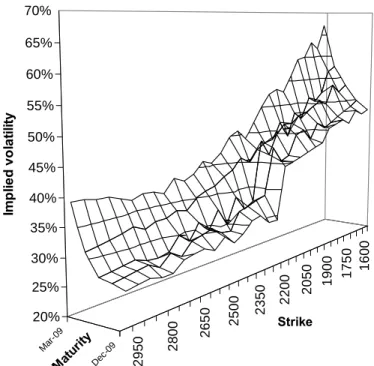
The advantages of the Black-Scholes model have been well known for years. The option price is expressed in closed form and the model is easy to implement. Nevertheless, the model assumes that continuously compounded stock returns are normally distributed with constant mean and variance. The assumption of constant volatility is very restrictive since a significant number of empirical studies show that volatility in asset prices is time-varying. In other words, this assumption contrasts with volatility smiles and smirks implicit in market option prices, as shown on Figure 1.
160 0 1750 1900 2050 220 0 235 0 2500 2 650 28 00 2950 Mar -09 De c-09 20% 25% 30% 35% 40% 45% 50% 55% 60% 65% 70% Im p lie d v o la tili ty Strike Matu rity
Figure 1: The volatility surface on 12-Fev-2009
for options on the Eurostoxx 50 stock index (with the spot price at 2214.95). Many of the advanced option pricing models have sought to overcome this assumption by incorporating time-varying volatility. The drawback of these models is that closed-form formulae are rarely available and the advantage of a more realistic description can be offset by the costs of implementation and calibration. Among such alternative models, stochastic volatility (SV) models
3
have attracted a great deal of interest because they manage to reproduce empirical regularities displayed by the risk-neutral density implied in option quotations. In this paper, we focus on the popular Heston (1993) model as well as on the Bates (1996) model which allows for the inclusion of jumps in the stock return dynamics.
The Black-Scholes model rests on the assumptions of uncorrelated and even independent asset returns. Although returns show little autocorrelation in most cases, they are usually not independent. In this respect, the Generalized Autoregressive Conditional Heteroskedasticity (GARCH) model is particularly useful for modeling volatility clustering in asset prices. It is therefore not surprising that researchers have attempted to incorporate GARCH effects into option pricing. Unfortunately, in most GARCH option pricing models, no closed-form analytic solution for the option price is available: the price is available only through Monte Carlo simulation. In this paper, we focus on the Heston and Nandi (2000) model for which a closed-form solution is proposed.
Finally, we compare these option-pricing models with a proprietary trading desk model developed by a leading European bank.
To the best of our knowledge, these five models (Black-Scholes, Heston, Bates, Heston-Nandi, and an internal model) have never been compared on both statistical and economic grounds during the Subprime crisis. In this paper, we use daily options prices on the Eurostoxx 50 stock index over the whole year 2008.
The paper is organised as follows. We briefly present the models in Section 2. We describe the data and the filter rules in Section 3. The calibration process is explained in Section 4. We carry out both in-sample and out-of-sample statistical analyses in Sections 5. The hedging performance of the models is described in Section 6. We conclude in Section 7.
4
2. Key features of the models
In general, the complexity of SV models raises severe implementation problems. However, the Heston model is well-known to stand out from the plethora of existing SV models due to its quasi-analytical closed-form solution. The Heston (1993) model diffusion process is described by
t t t t
t S dt S dz
dS =μ + ν 1,
where μis the drift parameter, νt is the instantaneous volatility, and z1,t is the wiener process. The instantaneous variance follows the following s.d.e.
,
[
t]
t tt K dt dz
dν = θ −ν +σ ν 2,
where K is the speed of mean reverting, θ is the long-run variance, and σ is the dispersion coefficient (the so-called vol-vol parameter). In this square-root diffusion model, νt is never negative provided that ν0, K, and θ are all positive. It
can also be shown that νt remains strictly positive if 2Kθ/σ2 ≥ 1 (Feller condition).
The two Wiener innovations are assumed to be correlated with
dt dz
dz
corr( 1,t, 2,t)= ρ
The effect of the σ parameter is to increase kurtosis of the stock return distribution while a negative correlation parameter ρ generates negative skewness. Nevertheless, some researchers and practitioners argue that the (constant) kurtosis and skewness introduced by stochastic volatility are not sufficient to correctly match market prices. For example, a purely diffusive
5
process seems not appropriate to explain the market quotes of deep out-of-the-money options with a few days before maturity.
One way to add flexibility to the model is by incorporating a jump process in to the stock dynamics to better account for the discrepancies between market prices/volatilities and those returned by the models. In this respect, the Bates (1996) model diffusion process is described by the following pair of s.d.e.
t t t t t t
t Sdt Sdz Jdn
dS =μ + ν 1, +
[
t]
t tt K dt dz
dν = θ −ν +σ ν 2,
whereJt is the jump size of a Poisson process and dntis the binary random variable equal to one with a probability of λ and zero with a probability of 1−λ (i.e. no jump). The correlation assumption between the two Wiener process is identical to Heston (1993). The inclusion of the jump process to the basic Heston model increases the magnitude of the smile for short term options. For the sake of simplicity, the jump process is uncorrelated with other processes (i.e. the underlying asset and variance processes), which may be questionable.
Finally, the Heston and Nandi model contribution lies in its discrete time assumption and the persistence in volatility that it captures. The model is calibrated on the underlying asset historical prices and not on option market data which may be illiquid. In the Heston and Nandi closed-form GARCH model for option pricing, the GARCH(1,1) forecast of volatility for time t + 1, based on values observed at time t, is given by
2 2
2
1 t t
t ω αr βσ
σ + = + + where 2
t
σ is the conditional variance and 2
t
r is the squared return. The variance
process of the Heston and Nandi model has been shown to converge towards the variance process of the Heston model when the time interval tends to zero.
6
3. Data and filter rules
We use options on the Eurostoxx50 stock index. The dataset covers the whole year 2008 on a daily basis and consists of 179,795 observations (89,676 calls and 90,119 puts) downloaded from Bloomberg. The risk free rate used in our simulation is the Euribor interest curve extracted from Bloomberg. To estimate the dividend rate, we use the future contract on Eurostoxx 50 dividend extracted from Bloomberg as well.
Most studies refer to the daily closing price (or mid-point of the bid-ask spread) as reflecting the value of the underlying asset on a daily basis. However, the use of daily closing prices is argued to increase the noise level, which tends to overprice options. We therefore use the volume weighted average price (VWAP) since VWAP has been shown to be statistically more efficient than the closing price.
In order to calibrate our models, we apply some traditional filter rules on the option data (Table 1). First, the option market prices must satisfy the no-arbitrage relationship (Merton, 1973). For example, the price for a call has to be greater than or equal to the spot price minus the present value of the remaining dividends minus the discounted strike price. Similarly, for a put, the price has to be greater than or equal to the present value of the remaining dividends plus the discounted strike price minus the spot price. Second, options with a volume of less than 10 contracts or with no open interest are considered as irrelevant. Third, options with a price lower than 0.375€/contract has been dropped to reduce the impact of price discretization. Fourth, options with an expiration date lower than 7 days have been excluded. Fifth, options with an expiration date longer than 1 year are rejected since they are less sensitive to volatility. Sixth, only the moneyness range (from 0.9 to 1.1) is considered since deeply out-of-the-money or in-the-out-of-the-money options are plagued by illiquidity issues. Finally, options with a bid-ask spread greater than 5% are excluded.
7
Outstanding call contracts 89.676
Criteria Rejected
No volume/open interest 47.296
Moneyness (<0.9;>1.1) 21.790
Bid-ask spread (<5%) 14.422
Maturity (>1 year) 11.990
Volume (<10 contracts) 1.707
Price (<0.375 €) 687
Maturity (<7 days) 539
No-arbitrage relationship 43
Rejected data 77.584
Remaining data 12.092
Filter results
Table 1: Filter rules.
Over 85% of our data has been rejected in the screening process. This restrictive data selection was driven by a concern to focus only on relevant data in order to reduce as much as possible illiquidity biases that may affect our final results. The remaining data set consists in 12.092 records and are well spread across moneyness and maturity, even though our sample slightly outweighs short run in-the-money calls with regards to long run out-of-the money calls (Table 2).
[0;90[ [90;180[ [180;270[ [270;360[
<0.94 246 (2.03%) 477 (3.94%) 524 (4.33%) 432 (3.57%) 1679 (13.89%)
[0.94;0.97[ 515 (4.26%) 483 (3.99%) 478 (3.95%) 419 (3.47%) 1895 (15.67%)
[0.97;1[ 644 (5.33%) 465 (3.85%) 457 (3.78%) 433 (3.58%) 1999 (16.53%)
[1;1.03[ 612 (5.06%) 443 (3.66%) 443 (3.66%) 432 (3.57%) 1930 (15.96%)
[1.03;1.06[ 546 (4.52%) 407 (3.37%) 418 (3.46%) 426 (3.52%) 1797 (14.86%)
1.06< 793 (6.56%) 643 (5.32%) 666 (5.51%) 690 (5.71%) 2792 (23.09%)
3356 (27.75%) 2918 (24.13%) 2986 (24.69%) 2832 (23.42%) 12092 (100%)
Maturity (days)
M
o
n
eyn
ess (
S
/K
)
8
4. Calibration
For the Heston and the Bates model, the calibration process consists in an inverse problem. We start from a parametric model which is supposed to drive the underlying asset price as best as possible and then we must find the parameters that minimize the discrepancies between the model and the market prices or volatilities. Choosing the appropriate loss function is a significant issue since each of the loss functions has some inherent flaws which may bias our results. We consider three widely-used loss functions: the Mean Absolute Error (MAE), the Mean Squared Error (MSE), and the Percentage Mean Squared Error (PMSE). The two traditional targets are the price and volatility discrepancies. The calibration results should theoretically converge towards the empirical volatility surface, that is, a leptokurtic distribution with a negative asymmetry and a slightly positive term structure. Nevertheless, the volatility surface has been impacted by the Subprime crisis in 2008, which may affect our parameters values.
We rely upon the widely-used lsqnonlin Matlab optimizer with the following initial parameters values. The current volatility and the long term volatility is set equal to the mean implied volatility observed on market data. The initial mean reversion rate was set at 3, the volatility of variance at 50%, and the correlation at -50%. For the Bates model, the starting jump parameters have a frequency of 0.2, a mean size of zero and a standard deviation of 30%. Boundaries were set in order to avoid inconsistent parameters values. The value of the correlation parameter is between -0.2 and -1, the volatility of variance is between 0 and 1, and the mean reversion rate is between 1 and 5. The jump is allowed to be either positive or negative as positive correlation has been found in our data sample.
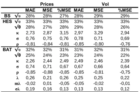
As expected, our parameters values depend on the loss function, even though the mean parameter values are quite homogenous (Table 3). The calibration process
9
in the Heston model (HES) captures the negative volatility term structure since the instantaneous volatility ( ν ) is higher than the long run volatility ( θ ). The correlation parameter (ρ) is also strongly negative in the option market (between -0.76 and -0.85). The volatility of variance (σ), the so-called ‘vol of vol’, ranges from 0.69 to 0.78 and the mean reversion rate (K) ranges from 2.73 to 3.29. The Feller condition is also fulfilled.
MAE MSE %MSE MAE MSE %MSE
BS √υ 28% 28% 27% 28% 29% 29%
HES √υ 33% 33% 33% 33% 33% 33%
√θ 28% 27% 28% 29% 28% 26%
κ 2,73 2,87 3,15 2,97 3,29 2,94
σ 0,76 0,75 0,76 0,78 0,71 0,69
ρ -0,81 -0,84 -0,81 -0,85 -0,80 -0,76
BAT √υ 32% 32% 31% 31% 32% 31%
√θ 25% 24% 23% 23% 24% 22%
κ 2,26 2,44 2,49 2,49 2,46 2,39
σ 0,74 0,71 0,67 0,67 0,66 0,64
ρ -0,85 -0,88 -0,85 -0,85 -0,81 -0,75
λ 0,26 0,21 0,26 0,25 0,25 0,22
mλ -0,02 0,01 -0,05 -0,05 -0,02 -0,01
σλ 0,19 0,16 0,13 0,13 0,13 0,12
Prices Vol
Table 3: Calibration on the whole data sample using different loss functions (BS: Black Scholes model; HES: Heston model; BAT: Bates model).
Loss Target BS HES HES/BS BAT BAT/BS
MAE Prices 1025,314 452,976 0,442 419,395 0,409
MSE Prices 31560,674 7514,349 0,238 7177,188 0,227
%MSE Prices 0,629 0,149 0,237 0,126 0,200
MAE Vol 1,691 0,684 0,405 0,630 0,373
MSE Vol 0,098 0,024 0,248 0,023 0,235
%MSE Vol 0,946 0,230 0,243 0,214 0,226
Table 4: Average loss functions values for different models (BS: Black Scholes model; HES: Heston model; BAT: Bates model).
The inclusion of the jump process in the Bates model (BAT) does not strongly affect the parameters values found for the Heston model. The parameters values of the Bates model are nevertheless lower than in the Heston model because part of the volatility is explained by the jump process. The frequency of the jump (λ) varies from 0.21 to 0.26 per year and the mean size of the jump (mλ) is typically
10
negative except for the loss function MSE on price where the jump is slightly positive (i.e. 0.01).
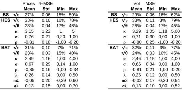
The MAE and MSE loss functions on prices tend to outweigh options that have a higher market value while the relative MSE on volatility deal with small values which push the Matlab optimizer to return less accurate results. Given the values of the different loss functions, we focus on two loss functions, namely the MSE on volatility and the %MSE on prices which deliver the lowest values. Some key descriptive statistics are given in Table 5.
Prices %MSE
Mean Std Min Max
BS √υ 27% 0,06 15% 59%
HES √υ 33% 0,10 10% 78%
√θ 28% 0,04 17% 46%
κ 3,15 1,22 1 5
σ 0,76 0,21 0,20 1,00
ρ -0,81 0,18 -1,00 -0,20
BAT √υ 31% 0,10 7% 71%
√θ 23% 0,03 15% 40%
κ 2,49 1,16 1,00 4,00
σ 0,67 0,29 0,14 1,00
ρ -0,85 0,16 -1,00 -0,34
λ 0,26 0,14 0,00 0,50
mλ -0,05 0,20 -0,39 0,60
σλ 0,13 0,15 0,00 0,70
Vol MSE
Mean Std Min Max
BS √υ 29% 0,06 16% 62%
HES √υ 33% 0,11 3% 79%
√θ 28% 0,04 17% 45%
κ 3,29 1,05 1,18 5,00
σ 0,71 0,30 0,00 1,00
ρ -0,80 0,25 -1,00 -0,20
BAT √υ 32% 0,11 3% 77%
√θ 24% 0,03 16% 45%
κ 2,46 1,15 1,00 4,00
σ 0,66 0,34 0,00 1,00
ρ -0,81 0,21 -1,00 -0,20
λ 0,25 0,12 0,00 0,50
mλ -0,02 0,17 -0,30 0,54
σλ 0,13 0,10 0,00 0,52
Table 5: Detailed parameters values over the whole sample data for the selected loss functions.
The standard deviations of key parameters, such as the correlation and the volatility of variance, are lower when the %MSE loss function on prices is relied upon. In addition, the minimum value of the volatility of variance parameter falls to zero when we use the MSE loss function on volatility. It may be more difficult for the Matlab local optimizer to find a good optimum based on the very small values delivered by the MSE loss function on volatility.
Time series graphs for the two key parameters of the basic Heston model (i.e. correlation and volatility of variance) can help us to choose the loss function that gives the most stable parameters values on a day to day basis (Figure 2). The
11
parameters display a more stable pattern and stick less often to the set boundaries with the %MSE loss function on prices. This confirms the superiority of the %MSE on prices over the MSE on volatility.
Volatility of variance (Prices %MSE)
0 0,2 0,4 0,6 0,8 1 1,2 0 50
100 150 200
Volatility of variance (Vol MSE)
0 0,2 0,4 0,6 0,8 1 1,2 0 50
100 150 200
Correlation (Prices %MSE)
-1,2 -1 -0,8 -0,6 -0,4 -0,2 0 0 50
100 150 200
Correlation (Vol MSE)
-1,2 -1 -0,8 -0,6 -0,4 -0,2 0 0 50
100 150 200
Figure 2: Time variation in correlation and volatility of variance for the selected loss functions in the Heston model.
The Heston and Nandi model has been calibrated using the Eurostoxx50 closing prices from January 1, 2008. The maximum likelihood estimates (MLEs) of the parameters and their corresponding key descriptive statistics are given in Table 5. In addition, the long term volatility has been found to be 18.33%, which is below the level obtained in the Heston and Bates models.
MLEs
Mean Std Min Max
HN α 1,14E-05 6,9E-06 3,76E-06 3,73E-05
β 0,793468 0,125296 0,607675 0,970487
γ* 102,5331 93,47525 0,5 278,1705
ω 1,14E-07 6,59E-07 4,14E-28 6,39E-06
σ2 t+1 0,000234 0,000191 2,75E-05 0,00116
Table 6: Detailed parameter values over the whole sample data for the Heston and Nandi model.
12
5. Statistical pricing performance
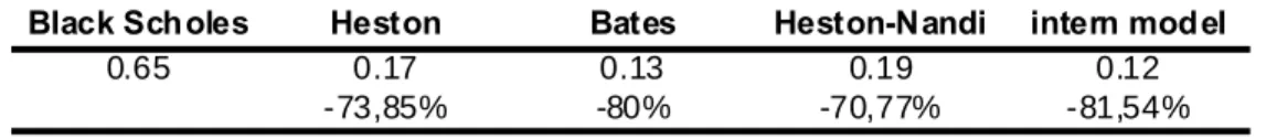
We first compare the in-sample performance of the SV models against two benchmarks, the Black and Scholes model and the internal model which is an improved version of the ad-hoc Black and Scholes.3 The mean parameters value
on the first six-month data was kept constant for the SV models and the internal model.
Black Scholes Heston Bates Heston-Nandi intern model
0.65 0.17 0.13 0.19 0.12
-73,85% -80% -70,77% -81,54%
Table 7: Average loss function value for the different models (up to July). The Black and Scholes model is clearly outperformed by the other models (Table 7). Among the SV models, the Heston and Nandi model displays the worst result. Although the calibration on option prices seems to be more accurate than the calibration on the underlying asset prices, the improvement does not seem to be very significant; probably because the volatility surface remained quite stable during the first six months of 2008. The best performing models are the Bates and the intern model.
In the out-of-sample test, all SV models have been updated weekly (Table 8). The models’ ranking remains the same. It is worth noticing that the Heston-Nandi model quality of forecasts drops, despite the parameters being updated weekly. This shows again that the calibration on the underlying asset data (backward looking) is not the most appropriate way to calibrate our model especially when the volatility surface evolves strongly. The other models performance is further improved by the parameters updating.
3 The ad-hoc Black-Scholes model (or Practitioner Black-Scholes model) constitutes a simple way
to price options, based on implied volatilities and the Black-Scholes pricing formula. The assumption of constant volatility is circumvented by using volatility that is not constant, but rather depends on moneyness and maturity. All that is required is a series of Black-Scholes implied volatilities on which to run multiple regressions under ordinary least squares.
13
Black Scholes Heston Bates Heston-Nandi Intern model
0.61 0.12 0.08 0.25 0.06
-80.33% -86.89% -59.02% -90.16%
Table 8: Loss function in the out-of-sample period (i.e. second half of 2008) Looking at the models performance during the highest volatility period, we notice that the Heston model and the Bates model perform better (Table 9). The Heston and Nandi model is strongly affected by the changing volatility surface and gets closer to the Black and Scholes results. The internal model still performs well but its relative performance deteriorates slightly when the volatility surface varies a lot.
Black Scholes Heston Bates Heston-Nandi Intern model
0.54 0.05 0.03 0.39 0.06
-90.74% -94.44% -27.78% -88.89%
Table 9: Loss function values during the high volatility period (from October to December).
In Table 10, we provide the loss function values for different maturities and moneyness. Short term (ST) options expire within 90 days; medium term (MT) options expire within 270 days and long term (LT) options expire in more than 270 days. In-the-money (IN) options have moneyness above 1.05. At-the-money (AT) options have moneyness between 0.95 and 1.05.Finally, out-of-the-money (OUT) options have moneyness below 0.95.
The performance of the Black and Scholes model seems to vary a lot in function of the moneyness and maturity. The highest loss function values are obtained for out-of-the-money short term options while the loss function values are lowest for long term in the money options. This confirms that the log-returns distribution tends to converge towards a normal distribution in the long run.
14
IN AT OUT
BS ST 0.38 0.89 1.25
MT 0.26 0.58 0.91
LT 0.19 0.23 0.27
HN ST 0.16 0.30 0.41
MT 0.10 0.14 0.20
LT 0.14 0.32 0.44
HES ST 0.13 0.13 0.11
MT 0.12 0.09 0.08
LT 0.07 0.09 0.10
BAT ST 0.06 0.07 0.06
MT 0.11 0.09 0.07
LT 0.08 0.10 0.07
INTERN ST 0.02 0.03 0.14
MT 0.03 0.02 0.07
LT 0 0.01 0.08
Table 10: Loss function values by maturity and moneyness.
The loss function values for the Heston model and the Bates model are better spread across maturity and moneyness. This indicates that the chosen loss function works well and do not favor any kind of options. As expected, the Bates model is superior to the Heston model especially for short term options.
The internal model performs quite well across all maturities and moneyness. Nevertheless, the loss function for short term out-of-the-money options might be further reduced by using the Heston or the Bates model.
6. Delta hedge performance in stress periods
The main contribution of the Heston models is often argued to lie in its delta hedge performance because the Heston delta takes into account the forecasted return distribution until the option matures.
In the following hedging application (Table 11), we hedge a short position of 10,000 option contracts. The hedge starts in July, 2008. The contracts are assumed to be sold at their market price so that the results are not affected by
15
the difference in pricing between the models. The implied volatility and the volatility process of all the models are defined at the beginning of the delta hedge and are held constant throughout the hedge. The hedging position is rebalanced daily.
Strike Market price IV BS HES HN
Put 2300 18,20 35,22% 2.887.284 2.902.469 3.929.427
Put 2400 25,30 34,38% 3.171.675 3.431.718 5.079.128
Put 2450 29,60 33,95% 3.091.141 3.352.889 5.946.911
Put 2500 34,50 33,52% 3.288.759 3.581.224 5.592.337
Put 2650 53,00 32,20% 3.529.977 3.811.130 4.795.255
Put 2700 60,70 31,76% 3.601.179 3.955.888 3.536.246
Put 2850 89,10 30,41% 3.830.650 4.169.647 1.983.158
Put 2900 100,50 29,95% 3.917.999 4.136.358 1.525.461
Put 3050 141,50 28,51% 4.318.010 4.154.736 6.346.229
Put 3150 175,20 27,52% 4.764.002 4.604.951 5.104.601
Put 3200 194,50 27,05% 5.052.926 4.970.250 4.897.416
Put 3300 238,10 26,16% 5.755.964 5.906.324 5.981.494
Put 3400 289,30 25,38% 6.624.615 6.977.646 5.763.539
Call 3400 134,80 22,27% - 714.715 - 1.172.326 54.850
Call 3350 157,20 22,69% - 776.430 - 1.182.589 - 854.492
Call 3300 181,60 23,11% - 922.726 - 1.175.572 - 1.207.800
Call 3250 207,80 23,52% - 1.029.409 - 1.151.286 - 1.154.849
Call 3200 235,80 23,93% - 1.144.332 - 1.140.262 - 1.016.049
Call 3150 265,50 24,33% - 1.182.729 - 1.157.235 - 1.617.593
Call 3100 296,80 24,72% - 1.327.433 - 1.256.854 - 3.060.548
Call 3050 329,50 25,08% - 1.468.906 - 1.483.948 - 3.551.439
Call 2900 435,30 25,94% - 1.988.499 - 427.5562.261.114
Table 11: Delta hedge performance of the Black and Scholes (BS), Heston (HES) and Heston and Nandi (HN) models.
(Options contracts taken as examples mature on 19-Dec-2008).
The delta hedge performance of the HN model is very volatile and does not follow the same path as the two other models. This would indicate that the HN model follows its own return distribution. Most importantly, the average performance of the HN model is better than the other models. This may be explained by the fact that the real return distribution does not display asymmetry during the period of the hedge.
The HES model outperforms the BS model for put options while the BS model outperforms the HES model for call options. This phenomenon is due to the fact that the HES model has a strongly negative volatility term structure.
16
Furthermore, the Heston model takes into account negative skewness which is temporarily not present in the return distribution.
In order to improve the performance of the HES model for out-of-the-money options contracts, we disregard the volatility term structure (Table 12). Indeed, the hedging performance deteriorates because of the strongly negative term structure (and a very high initial variance) in the Heston model which in turn increases the delta of the Heston model.
Strike Market price IV BS HES
Put 2300 18,20 35,22% 2.887.284 3.988.955
Put 2400 25,30 34,38% 3.171.675 4.437.142
Put 2450 29,60 33,95% 3.091.141 4.867.430
Put 2500 34,50 33,52% 3.288.759 5.284.608
Put 2650 53,00 32,20% 3.529.977 5.648.393
Put 2700 60,70 31,76% 3.601.179 4.529.766
Put 2850 89,10 30,41% 3.830.650 4.933.917
Put 2900 100,50 29,95% 3.917.999 5.522.130
Put 3050 141,50 28,51% 4.318.010 6.790.409
Put 3150 175,20 27,52% 4.764.002 6.487.030
Put 3200 194,50 27,05% 5.052.926 5.647.471
Put 3300 238,10 26,16% 5.755.964 5.992.915
Put 3400 289,30 25,38% 6.624.615 7.054.343
Call 3400 134,80 22,27% - 714.715 - 64.821
Call 3350 157,20 22,69% - 776.430 - 647.986
Call 3300 181,60 23,11% - 922.726 - 929.710
Call 3250 207,80 23,52% - 1.029.409 - 801.696
Call 3200 235,80 23,93% - 1.144.332 - 872.103
Call 3150 265,50 24,33% - 1.182.729 - 992.518
Call 3100 296,80 24,72% - 1.327.433 - 1.261.741
Call 3050 329,50 25,08% - 1.468.906 - 341.575
Call 2900 435,30 25,94% - 1.988.499 246.130
Table 12: Delta hedge performance of the Black and Scholes (BS) model compared to the Heston (HES) model disregarding the volatility term structure. By cancelling out the effect of the term structure, the hedging performance of the Heston model is improved for contract that matures out-of-the-money. Overall, these results converge with the study of Bakshi et al. (1997) carried out in normal market conditions: the Heston model outperforms the Black and Scholes model in terms of hedging errors, mainly for option contracts that mature in-the-money.
17
7. Conclusion
We show that stochastic volatility (SV) models outperform the Black and Scholes model in stress periods. By using SV models, correlation between the underlying asset price and the volatility is taken into account, which is helpful in capturing skewness. In addition, SV models incorporate the volatility of variance that captures the kurtosis through the variance process. These parameters allow fitting the smile observed in the options market.
The Heston, Bates, and Heston-Nandi models are complements, rather than substitutes. The Bates stochastic volatility model with jumps is better adapted to short term options because of the steeper skewness. Given their flatter volatilities, medium or long term options are better treated by the Heston or the Heston and Nandi stochastic volatility model. Finally, although the SV models do not significantly outperform the internal model, their relative performance in stress periods improves.
The SV ‘Heston-type’ models provide quasi-analytical solutions and offer a good compromise between accuracy and computational time. However, no standard calibration procedure still exists and the volatility surface may be inconstant through time which makes calibration challenging in stress periods.
For pricing purposes, the Black and Scholes model could be adjusted by applying the implied volatility extracted from the options market prices, also known as ad-hoc Black and Scholes or Practitioner Black and Scholes model. Nevertheless, this model should be used while keeping in mind that no variance process is defined so that the underlying assumptions of the Black-Scholes model still hold, i.e. the normal distribution and the constant volatility. The model is just lined up to market prices observed at a certain point in time.
In terms of pricing, the Heston model harbours several interesting aspects but those improvements remain more theoretical than practical. Indeed, the ad-hoc
18
Black and Scholes model remains widely used in practice because it fits the market prices without requiring any calibration.
The main contribution of the Heston and Nandi model lies in its delta hedge performance. The definition of a variance process allows forecasting the expected return distribution of the option contracts which cannot be achieved by the (ad-hoc) Black and Scholes model. This remains true in periods of heightened pressure.
References
Bakshi, G., Cao C. and Chen Z. (1997), Empirical performance of alternative option pricing models, Journal of finance 52, 2003-2049
Bates, D. (1996), Jumps and Stochastic Volatility: Exchange Rate processes Implicit in Deutchemark Options, Review of Financial Studies 9, 69-107.
Heston, S. (1993), A Closed-Form Solution for Options with Stochastic Volatility, Review of Financial Studies 6, 327-344.
Heston S. and Nandi, S. (2000), A closed-form GARCH option valuation model, Review of Financial Studies 13, pp585-625