C.S. Jensen et al. (Eds.): EDBT 2002, LNCS 2287, pp. 197–214, 2002. © Springer-Verlag Berlin Heidelberg 2002
Myoung-Ah Kang1, Christos Faloutsos2
, Robert Laurini1, and Sylvie Servigne1 1 LISI, INSA de Lyon-Lyon Scientific and Technical University
20 Av.Einstein 69621 Villeurbanne, France
{makang, laurini, servigne}@lisi.insa-lyon.fr
2 Dept. of Computer Science, Carnegie Mellon University Wean Hall , 5000 Forbes Avenue, Pittsburgh, PA 15213-3891
Abstract. With the extension of spatial database applications, during the last
years continuous field databases emerge as an important research issue in order to deal with continuous natural phenomena during the last years. A field can be represented by a set of cells containing some explicit measured sample points and by arbitrary interpolation methods used to derive implicit values on non-sampled positions. The form of cells depends on the specific data model in an application. In this paper, we present an efficient indexing method on the value domain in a large field database for field value queries (e.g. finding regions where the temperature is between 20 degrees and 30 degrees). The main idea is to divide a field into subfields [15] in order that all of explicit and implicit val-ues inside a subfield are similar each other on the value domain. Then the in-tervals of the value domain of subfields can be indexed using traditional spatial access methods, like R*-tree [1]. We propose an efficient and effective algo-rithm for constructing subfields. This is done by using the field property that values close spatially in a field are likely to be closer together. In more details, we linearize cells in order of the Hilbert value of the center position of cells. Then we form subfields by grouping sequentially cells by means of the cost function proposed in this paper, which tries to minimize the probability that subfields will be accessed by a value query. We implemented our method and carried out experiments on real and synthetic data. The results of experiments show that our method dramatically improves query processing time of field value queries compared to linear scanning.
1 Introduction
The concept of field has been widely discussed for dealing with natural and environ-mental continuous phenomena. Field data have a great impact in GIS to describe the distribution of some physical property that varies continuously over a domain. A typical example is altitude over a two-dimensional domain to describe a terrain. Other examples of two-dimensional fields are distributions of temperature, pressure, pollu-tion agents, etc., over the surface of a territory. Three-dimensional fields can model geological structures and, in general, physical properties distributed in space. These
involve large data set and their analysis. The technology of field databases serves as an important bridge for extending spatial database to scientific databases.
A field can be defined as a function over space and time from a mathematical point of view. Field data are either scalar or vectorial depending on the result of the corresponding function. When the result is of single value, such as the temperature at a point, the field becomes scalar. On the other hand, the field is vectorial, when the result is of multiple values (for instance wind). And the most common queries for analyzing field data can be divided into two categories as follows :
1. Queries based on a given position: e.g. what is the value at a given point p ? 2. Queries based on a given field value: e.g. what are the regions where the rainfall is
more than 2000 mm per year ?
The first type of queries is to find the field values at a given position. On the other hand, the second type, which is more difficult than the first type, inquires the regions, where the field has a given value. We term the second type of queries as field value queries in contrast to conventional queries of first type of queries. Although the two types of queries are related with field, their processing methods are different and the processing cost is expensive due to the large volume of data. The processing of the field value queries are more difficult and expensive with comparison to the conven-tional queries. There is no proposed indexing method for field value queries to our knowledge even though the conventional queries can be supported by a existing spa-tial indexing method. By contrast, in many applications, field value queries are important for the analysis. Specific applications include the following :
− In ocean environmental databases with ocean temperature and salinity field data, suppose that salmons can be found in the part of sea under a certain condition of temperature and salinity. The queries we can ask for fishing salmons would be "Find regions where the temperature is between 20° and 25° and the salinity is be-tween 12% and 13%".
− In the urban noise system, a typical query to know the noisy regions would be "Find regions where the noise level is higher than 80 dB ", where dB is an unit of noise level.
Despite the importance, no significant attention has been paid and no remarkable work has been done on the indexing and query processing for field data. Although a certain amount of researches are found, they still focus on the representation or mod-eling issues for field. Most of the researches deal with the issues of the representation of continuous fields and appropriate data models [16, 20, 25]. In [10] an object ori-ented model to implement a new estimation method for field data has been specified and the refined object oriented model which permit to change dynamically the estimation method has been studied.
The goal of this paper is to design of indexing methods for efficient field value queries processing in large field databases. The proposed indexing methods exploit the continuity of field, which is an important property of field. And our methods are based on the division of a field into several subfields in the context of the homogene-ity of field values. The notion of subfield allows an approximate search in the level of subfields instead of the exhaustive search on the entire field, by discarding non-qualified subfields for a given search condition.
The organization of this paper is as follows. In section 2, we will introduce the field representation, the overall procedures of query processing in field databases. In particular, the difficulties of query processing of field value queries will be presented in that section. In section 3, the concept subfield [15] will be introduced and we will show how to use it for indexing field values. Then, we will define two aspects to consider in order to determine subfields in the given field. We will propose a new indexing method defined by these two aspects so that the indexing method could be adaptable to the distribution of data and could try to minimize the number of disk accesses. We present results of some experiments not only on real data but also on synthetic data generated by a fractal method, which show the improvement of the performance by using our indexing methods in section 4. And we conclude our paper in section 5.
2 Field Databases and Related Work
2.1 Field Representation
In many cases, the phenomenon under consideration can not be sampled in every point belonging to the study area: for example groundwater, temperature. Instead, the sample dataset is measured or generated at some points or in some zones and the spatial interpolation methods are used in order to estimate the field value at not sam-pled locations. A field based on a sample point dataset can be formally modeled as follows :
A sample dataset in a field of d-dimension is a pair of (V,W), where V = {vi∈ R d
, i=1,…, n} is a finite set of points in a domain Rd, in which integer d represents the dimension of the domain, i.e., R3 for a 3-d dataset V which is a set of points with a coordinate (x, y, z) or R4 for 3-D spatial and 1-D temporal domain with coordinate (x, y, z, t). And W = {wi∈ R
k
, i=1, …, n} is a corresponding set of field values ob-tained by wi = F(vi), in which F is the interpolation function and the integer k
de-cides if the field is scalar or vector, thus if k = 1 then scalar field, or if k >= 2 then vector field respectively. A continuous field with a dataset (V, W) is by a pair (C, F), where C is a subdivision of the domain Rd
into cells ci (c1, c2, …, cn) containing some points of V, and F is a set of corresponding interpolation functions fi (f1, f2, …,
fn) of cells; fi represents the corresponding cell ci, which means that it is possible to define some different interpolation methods to represent a field, if necessary. A scalar field has a single value at every point, i.e., temperature, land surface ele-vation or noise level. By contrast, a vector field has a vector rather than a single value, i.e., the gradient of the land surface (aspect and slope) or wind (direction and magnitude). In this paper, we only consider scalar fields.
Cells can be of regular or irregular form and the number of sample points con-tained by a cell can vary even in a field space, i.e., regular square in DEM (grids, Digital Elevation Model) or irregular triangle in TIN (Triangulated Irregular Net-works), or hybrid model of hexahedra or tetrahedra in a 3-D volume field. In most
cases, the sample points contained by a cell (we term these points as sample points of cell) are vertices of the cell like the models DEM, TIN, etc.. However we do not ex-clude the possibility to have sample points inside a cell for a certain interpolation method in the case of necessity such as the Voronoi interpolation.
The function fi is used to interpolate field values of all the points inside cell ci by
applying fi to the sample points of cell ci . The reason is that the sample points of a cell
are generally the nearest neighbor points of the given query point and the field value on a point is influenced principally by the nearest sample points by the field continu-ity property. For example, in the 2-D TIN with a ‘linear interpolation’, we take three vertices of the triangle containing the given point to apply the function.
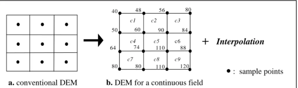
A conventional raster-based DEM for imagery is not suitable to represent a con-tinuous field. Because it defines just one value (i.e., the terrain elevation measured in the center of cell) for all points inside a cell, which means the lost of the all within-cell variation [20] and the discontinuity between adjacent within-cells. In order that a DEM can be considered as a continuous field, interpolation methods need to be specified [26]. To meet this condition, we can generate (measure) sample points at each vertex of grid and specify an interpolation function, i.e., a linear interpolation. Thus all the points inside a cell can be interpolated by their nearest neighbor sample points, so that their vertices of the cell. Figure 1 illustrates an example of the transformation of a conventional DEM to the DEM for a continuous field such as a terrain.
Fig. 1. Example of a DEM for continuous fields
2.2 Queries on Field Databases
For simplicity we assume the interpolation function f as a linear interpolation in all the illustrating examples in this paper. Note that the approaches in this section can be applied to other interpolation methods as well. Depending on different query condi-tions we can classify the type of queries in field databases as follows :
− Q1 : Queries based on a spatial condition, i.e., Find field value on a given point v'.
− Q2 : Queries based on a field value condition, i.e., Find regions with a given field value w'.
Complex queries can be composed by combining these basic queries. 40
c1
48 56 80 50 60 90 84
88 120 110 80 80
64 74 110 c6
c2 c3
c4 c5
c7 c8 c9
a. conventional DEM b. DEM for a continuous field
+
Interpolation2.2.1 Conventional Queries. The type Q1 is the conventional query type in field
databases, denoted as F(v’). It returns the field value on a given point v', i.e., “what is the temperature on a given point v'?”. To process this type of queries, we find firstly the cell c’ containing the query point v' and we apply the corresponding interpolation function on the neighbor sample points of the query point v', namely samples points of the c’ retrieved in the previous step ; w' = f(v', sample_points(c’)). Therefore the problem in a large field database is to efficiently find the qualified cell c’. This is one of the traditional spatial operations in spatial databases. Thus these queries can be easily supported by an conventional spatial indexing method, such as R-tree or its variants [1, 12, 23].
2.2.2 Field Value Queries. The type Q2 is to find the regions with a given field
value w'. The query condition value w’ involves not only exact match conditions but also range conditions. For example, a range query such as “Find the regions where temperature is between [20oC, 25oC]” or “Find the regions where temperature is more than 25oC” belongs to this query type. Most applications of field databases do not really care about “where are the value exactly equal to w' ?”, instead they are interested in the queries such as “where are the value approximately equal to w' ?”, since errors and uncertainty exist in the measurements. These queries can be denoted as F-1(w’-e < w < w’+e) where e is an error limit. More generally, they can be denoted as F-1(w’ < w < w”), which is a range query.
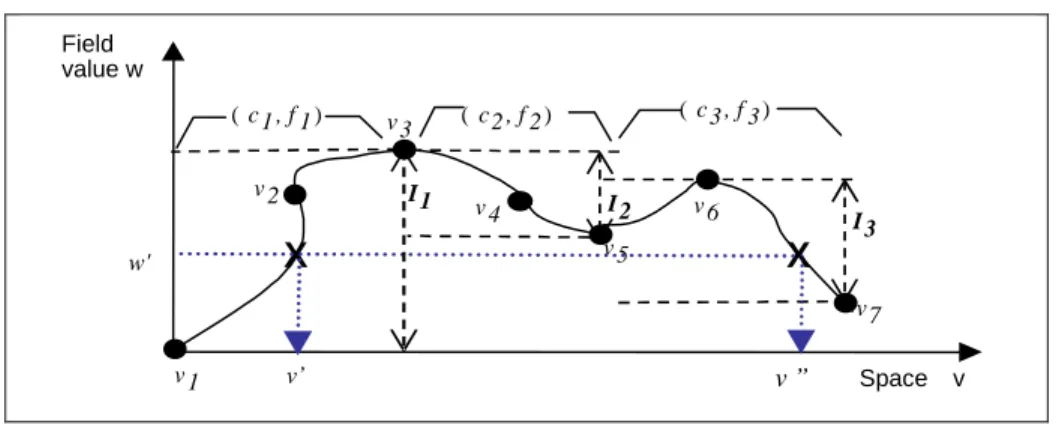
Compared with the type Q1 queries, value queries are more difficult to support since there can be more than one cell where the field value is equal to (larger than, smaller than) w’. Figure 2 illustrates an example of a value query in a 2-D continuous field. Note that the spatial XY plan is simplified to the axis ‘Space v’ in this figure to show intuitively the value queries processing procedure. The field is viewed as con-tinuous from their sample points and interpolation functions. The cell c1 contains
sample points <v1, v2 ,v3 > and it is represented by an interpolation function f1. The cell
c2 contains <v3, v4, v5> and it is represented by f2, respectively, etc. We can remark that
the sample points of each cell support implicitly the interval of all possible values inside a cell ; not only explicit sample values and also implicit values to be interpo-lated. These intervals are represented by Ii for the cell ci in Figure 2.
In Figure 2, the answer points where the field value is equal to the query value w’ are v’ and v”. These answer points can be calculated by interpolation if we can re-trieve all cells <c1, c3> whose intervals intersect the query value w’. In detail, v’ can
be calculated by applying the inverse interpolation function on the sample points of c1, namely <v1, v2, v3> ; f1
-1
(w’, sample_points(c1)). And v” can be done by the function
f3-1 on the sample points of c3 <v5, v6, v7> ; f3 -1
(w’, sample_points(c3)). In the same way,
in Figure 1, for a given query such as “Find the regions where the value is between 55 and 59”, firstly we need to retrieve the cells <c1, c2, c3, c4>, whose intervals intersect
the range query value [55, 59]. Then, the final exact answer regions can be retrieved by applying the inverse function on the vertices of each cell retrieved in previous step.
Fig. 2. Example of a continuous field and a value query
Thus, the problem of value queries in a continuous field database is transformed into the problem of “finding all the cells whose value intervals intersect the given query value condition”. Without indexing, we should scan all cells of the database, which will degrade dramatically the system performance. We term this method as ‘LinearScan’ method. Thus in this paper, we propose an efficient indexing method to support value queries in large continuous databases by accelerating the retrieval of all the cells intersecting a query value condition w’. We should point out that if the inter-polation function introduces new extreme points having values outside the original interval of cells, these points must be considered when deciding intervals of cells.
2.3 Related Work
The similar approaches of the value query processing have been proposed for isosur-face extraction from volumetric scalar dataset [4] and for the extraction of isolines from TIN [24]. Thus each volume or triangle is associated with an interval bounded by the elevation of the vertices of the cell (volume or triangle) with lowest and high-est elevation. For any query elevation w' between this interval (the lowhigh-est and the highest elevation), the cell contributes to the isosurface or isoline map. An Interval tree [5] was used in order to index intervals of cells for intersection query. However, the Interval tree data structure is a main-memory based indexing method thus it is not suitable for a large field database.
In [19], IP-index [18] for indexing values of time sequences was used for the ter-rain-added navigation application. The IP-index was applied to the terrain elevation map of DEM to find area whose the elevations are inside the given query interval. Since the IP-index is designed for 1-D sequences, an IP-index was used for each row of the map by considering it as a time sequence. This approach could not handle the continuity of terrain by considering only the continuity of one dimension (the axis X).
w'
v’ v ”
X
X
I1 I2
I3
v 1 v 2
v 3 v 4
v 5 v 6
v7 Field
value w
Space v
2.4 Motivation
As we saw before, without indexing value query processing requires to scan the entire field database. Despite the importance of the efficient value query processing, no significant attention has been paid and no remarkable work has been done on the indexing methods. In this paper, we would like to build new indexing schemes which can improve the value query processing with in large field databases. This is the mo-tivation of this paper.
3 Proposed Method
As mentioned above, the problem of answering value queries translates to finding a way to index cells intersecting the query value. Given a field database, we can associ-ate with each cell ci an interval, whose extremes are the minimum and maximum
value among all possible values inside ci, respectively. One straightforward way is
therefore to index all these intervals associated with the cells. An interval of values represents the one dimensional minimum bounding rectangle (MBR) of values that it includes. Thus we can use 1-D R*-tree to index intervals. We term this method as ‘I-All’ method, where I represents ‘Indexing’. Given a query value w’, we can search the 1-D R*-tree in order to find intervals intersecting w’. Then we retrieve the cells asso-ciated with found intervals and we calculate the final exact answer regions by the interpolation method with sample points of retrieved cells. Because these cells corre-spond to cells containing a part of answer regions. We term these cells as candidate cells. However storing all these individual intervals in an R*-tree has the problems as follows:
The R*-tree will become tall and slow due to a large number of intervals in a large field database. This is not efficient both in terms of space as well as search speed. Moreover the search speed will also suffer because of the overlapping of so many similar intervals. Sometime they lead to more poor performance than the ‘Linear-Scan’ method as we can see in Figure 11.a in Section 4.
Thus we propose an another efficient method based on the continuity of field, which is an important property of field concept. By the continuity property, the values close spatially in a continuous field are likely to be closer together. It means that the adjacent cells probably become the candidate cells together for a given query.
Therefore we propose to group these (connected) adjacent cells having similar val-ues into subfields. Since a field is entirely covered by a set of cells, subfields mean also a division of a entire field space into some subspaces. Thus a subfield can be defined as a subspace where field values are close together. Then we can get the in-tervals of all possible values inside subfields instead of individual inin-tervals of all cells, and we can index only these a few intervals of subfields by using 1-D R*-tree. It means that a value query firstly retrieves the subfields whose intervals intersect the query value by R*-tree. It is evident that if a value query intersects some intervals of cells inside a subfield then it has to intersect also the interval of subfield itself. The
final exact answer regions need to be calculated by interpolating the cells inside re-trieved subfields. The i-th subfield can be defined by its interval as follows :
SFi = (Wmin,i , Wmax,i ) ,
where Wmin,i and Wmax,i mean the minimum and maximum value of values inside SFi,
respectively.
We may append other kinds of values to Vmin,i and Vmax,i , if necessary, for example,
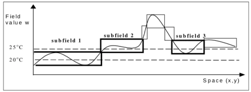
the average of field values of subfield. Figure 3 shows an example of the division of a continuous field into some subfields. The spatial XY plan is simplified on the axis 'Space (x,y)'. In this figure, subfields are represented by rectangles. It means that each rectangle contains (or intersect) some adjacent cells that are not drawn in this figure for the simplicity. The width of rectangle implies the area of subfield covering some cells. The height of rectangle does the interval of subfield. Note that these heights are not very large since the values inside subfields are similar each other. In other words, the similarity of values inside a subfield can be represented by the interval size of the subfield, which means the difference between maximum and minimum value inside.
s u b f i e l d 3 s u b f i e l d 2
s u b f i e l d 1
2 5o C 2 0o
C
F ie ld v a lu e w
S p a c e ( x , y )
Fig. 3. Indexing for field value queries with subfields
Since we use 1-D R*-tree with these intervals of subfields, the procedure of value query processing can be defined as follows :
• Step 1 (filtering step) : find all subfields whose intervals intersect the query value by the R*-tree.
• Step 2 (estimation step) : retrieve all cells inside the selected subfields by step 1, and estimate the exact answer regions where the value is equal to (more than or less than) the query value.
Suppose that a TIN is used to represent the field in Figure 3 and that a query such as “Find the zone where temperature is more than 20o
C and less than 25o
C” is given. For the filtering step, we select three subfields 1, 2, and 3, which intersect query in-terval. And we retrieve the triangles contained or intersected by the selected subfields and compute the regions where the temperature is between [20o
C, 25o
C] with the sample points of retrieved triangles.
3.1 Insertion
Before insertion of intervals of subfield in 1-D R*-Tree, we have to define how to get these subfields for indexing for value queries. How can we divide a field space into some subfields so that these subfields could have the similar values ?
3.1.1 Subfields. In order to get subfields, we must consider two aspects so that the
number of disk accesses can be minimized.
1. The manner to divide the field space : It means also how to group some (con-nected) adjacent cells into subfields, since a field space is totally covered by cells. 2. The criterion of similarity of values inside a subfield : As we saw before, we can
use the interval size of subfield as a criterion of measurement of similarity of val-ues inside a subfield.
In the paper [15], Interval Quadtrees have been proposed. The division of space is based on that of Quadtree [22]. And they used a pre-determined, fixed threshold for the interval size of subfield. It means that the interval size of a subfield must be less than the given fixed threshold in order that values inside are similar. In detail, the field space is recursively divided into four subspaces in the manner of Quadtree until each subspace satisfies the condition that interval size of the subspace must be less than the given threshold. Then the final subspaces of this division procedure become subfields. However, there is no justifiable way to decide the optimal threshold that can give the best performance. And the quadratic division is not very suitable to a field represented by non quadratic forms of cells such as TIN. Thus we would like to find a method that will group cells in order that subfields could have more natural and realistic forms by trying maximum of adjacent cells. It means no limitation of forms quadratic or triangular, etc., like in the case of Interval Quadtree. We propose to use a space filling curve to impose a linear ordering on the cells covering a field space. We term this method as 'I-Hilbert'.
3.1.2 The Manner to Divide the Field Space Using Hilbert Value Order. A
space filling curve visits all the points in a k-dimensional grid exactly once and never crosses itself. The Z-order (or Peano curve, or bit-interleaving), the Hilbert curve, and the Gray-code curve [6] are the examples of space filling curves. In [7, 13], it was shown experimentally that the Hilbert curve achieves the best clustering among the three above methods. Thus we choose the Hilbert curve. Indeed, the fact that all successive cells in a linear order are the adjacent cells each other in k-dimension; there is no “jumps” in the linear traversal, allows to examine sequentially all cells when generating subfields.
The Hilbert curve can be generalized for higher dimensionalities. Algorithms to generate two-dimensional curve for a given order can be found in [11, 13]. An algo-rithm for higher dimensionalities is in [2]. Figure 4 shows examples of the Hilbert curve ordering.
Fig. 4. Example of Hilbert curves
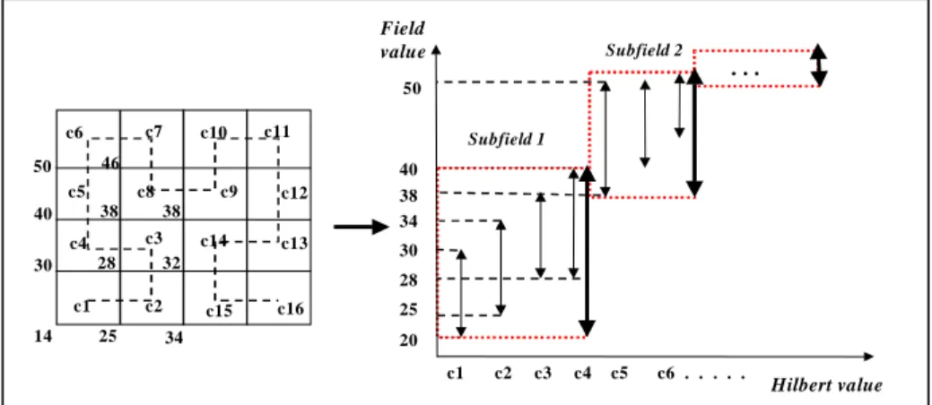
The cells will be linealized in order of the Hilbert value of their spatial position, specifically the Hilbert value of the center of cells (from now, in this paper the Hilbert value of a cell means that of the center of the cell). Then we check sequentially inter-vals of linealized cells if their values are similar or not in order to generate subfields. Therefore, each cell can be represented only by its interval in the procedure of sub-fields generation like in the Figure 5.b. Figure 5.a presents an example of a continu-ous field represented by a regular DEM and Figure 5.b shows some subfields gener-ated according to the intervals of cells.
Fig. 5. : a. Example of continuous DEM, b. Generated subfields and their intervals
Data Structure of subfields As mentioned above, each interval of subfields shown
in Figure 5.b can be indexed by 1-D R*-tree storing it in a 1-D MBR. We should point out that at the leaf nodes of the R*-tree, we need to store disk addresses where cells within the corresponding subfield are stored. The adjacent cells in subfields are already clustered by linealiring them physically in order of Hilbert value of cells. Therefore it is sufficient to store the pointers of starting and ending cells of the sub-field in the linear Hilbert value order. Figure 6 shows the structure of a leaf node and a non-leaf node of 1-D R*-tree for intervals of subfields.
14 28 30 25 38 38 40 32 Field value Hilbert value 20 30 25 40 c1 c9 c3
c1 c2 c3 c4 c5 c8
c2 c5
c7
c4
c6 c10 c11
c12 c13 c15 c14 c16 34 34 38 28
c6 . . . . .
. . . Subfield 1 Subfield 2 50 46 50 3 1 2 0 3 4
5 6 9 10
11 12 15 0 7 8 2 13 1 14 H 3 H1 H2
Fig. 6. Data structure of nodes of 1-D R*-tree for intervals of subfields
Before describing the cost function, we define an interval size of a cell or that of a subfield having minimum and maximum values as,
interval size I = maximum-minimum + 1.
In the special case that the minimum and maximum value are the same, for exam-ple when a interpolation function returns a constant value for all points in a cell, the interval size is 1. According to [14], the probability P that a subfield of interval size L, that is, an 1-D MBR of length L will be accessed by the average range query is :
P = L + 0.5
It assumes that the data space is normalized to the range [0,1] and that average range query is of length 0.5. Then we define the cost C of the subfield as followings :
C = P / SI,
where SI is the sum of interval sizes of all cells inside the subfield. Namely, the prob-ability of accessing a subfield is divided by the sum of interval sizes of cells included by the subfield.
The strategy is that the insertion of the interval of a new adjacent cell into a sub-field containing already some cells must not increase the cost C of the subsub-field before the insertion. Suppose that Ca be the cost of a subfield before the insertion of a new
cell and Cb after the insertion, respectively. This insertion can be executed only if Ca
> Cb. Thus at first, we start with the interval of first cell of the whole linearized cells. Then we form a subfield by including all the successive cells until the cost of subfield before insertion of a cell Ca is more than that of the subfield after intersection Cb. In
the case of Ca <= Cb, we start a new subfield. In this way, subfields are generated by
including sequentially cells in a field. For example, in Figure 5.b the cost of Subfield 1 before the insertion of cell c5 into Subfield 1 was about 0.466; 21/(11+10+11+13). The cost of Subfield 1 after this insertion will be about 0.534; 31/(11+10+11+13+13). This insertion increased the cost of Subfield 1 before insertion, thus a new Subfield 2 was started with c5.
Figure 7 shows an example of the sub-fields generated by the proposed method above with real terrain data of a part of ROSEBURG city in USA obtained at http://edcwww.cr.usgs.gov. The areas of subfields are represented by polygon on the map where the terrain elevations are represented by different colors.
… min, max ...
min, max
…
ptr_start, ptr_end ... b) leaf levela) non leaf level
Fig. 7. Examples of generated subfields
3.2 Search
In the previous subsection, we showed how to construct 'I-Hilbert' indexing method. Here we examine how to search the index for value queries. The searching algorithm starts to perform a intersect query within the 1-D R*-tree constructed by intervals of subfields. It retrieves all leaf MBRs intersecting the given query field value then es-timate the exact answer regions by retrieving cells located between the pointers of starting and ending cell.
Algorithm Search(node Root, query value w) :
S1. Search non-leaf nodes : invoke Search for every entry whose MBR intersects the query value w.
S2. Search leaf nodes : invoke Estimate(ptr_start, ptr_end, w) of every entry whose MBR intersects the query value w.
Algorithm Estimate(pointer ptr_str, pointer ptr_end, query value w) :
E1. Retrieve sample points of cells at the disk ad-dress between ptr_str and ptr_end.
E2. Estimate the exact answer regions corresponding
to w with retrieved sample points.
4 Experiments
We implemented the our method 'I-Hilbert' and we carried out experiments on two spatial dimensional field data. The method was implemented in C, under Unix. We compared our method against the ‘LinearScan’ and ‘I-All’ methods. For each ex-periment, we used interval field value queries with variable query intervals :
Qinterval : ranged from 0-0.1 relatively to the normalized interval range of the to-tal field value space to [0, 1]. For example, interval value queries ranged 0 mean exact field value queries such that “Find all regions where the value is equal to 30“.
We generated randomly 200 interval field value queries for each query interval Qinterval. We measured the execution time of field value queries by calculating the average of total query processing time of these 200 queries. The page size used is 4KB. Both real and synthetic data were used in the measurement. The reason for using real data was to evaluate how the our method behaves in reality. We used syn-thetic data by controlling several parameters of field data in order to test our method on larger and various types of data. A simple linear interpolation was used for inter-polating all the points inside a cell for every kind of data.
4.1 Real Data
Two kinds of real field data were used as followings :
1. Real terrain data : The USGS DEM elevation data of a region in USA was ob-tained from http://edcwww.cr.usgs.gov. Their resolution was 512*512, so 266,144 rectangular cells having four vertexis in the field space. Figure 8.a shows the re-sults of performance comparison of 'I-Hilbert' against the ‘LinearScan’ and ‘I-All’ methods.
2. Real urban noise data : A real urban noise data measured in a region of Lyon, France were used. The noise data were represented by TIN with about 9000 trian-gles. Figure 8.b shows the results of performance according to varied field value query interval.
Fig. 8. Execution time of field value queries with the real data
Our method 'I-Hilbert' outperforms 'LinearScan' and 'I-All' methods with the ter-rain data and also urban noise data. Our method achieves from 6 up to 12 times better query processing time than 'LinearScan' method in Figure 8.a.
4.2 Synthetic Data by Fractal
We used synthetic data of various characteristics. As synthetic field data, we gener-ated 2-D random fractal terrain of DEM by the diamond-square algorithm using the midpoint displacement algorithm as random displacements [21]. Thus an height of terrain at each vertex is generated. In the diamond-square algorithm, we start out with a big square and initial heights chosen at random at the four vertices. The square grid is subdivided recursively into the next with half grid size by one pass consisting of two steps, see Figure 9 :
− The diamond step : The midpoints of all squares are computed by interpolation from their four neighbor points (average of four neighbor points) plus an offset by the random displacement.
− The square step : The remaining intermediate points are computed by interpolation from their four neighbor points plus an offset by the random displacement.
a. real terrain data b. real urban nose data 0,00
2,00 4,00 6,00 8,00 10,00 12,00 14,00
0 0.02 0.04 0.06 0.08 0.1 Qinterval
Execution time(ms)
LinearScan I-All I-Hilbert
0 0,05 0,1 0,15 0,2 0,25 0,3 0,35 0,4 0,45
0 0.02 0.04 0.06 0.08 0.1 Qinterval
Execution time(s)
LinearScan I-All I-Hilbert
Fig. 9. Two passes of subdivision for generation fractal surfaces by diamond-square
algorithm on a square of 4 x 4
The midpoint displacement algorithm is used as random displacement for generat-ing an offset. Therefore when we assumes that value space (heights of terrain) is normalized to [-1.0, 1.0], the initial random value range from [-1.0, 1.0]. In each pass, an offset is randomly generated in the random value range in each of two steps and then the random value range is reduced by the scaling factor of 2(-H)
.
The H is a parameter for the roughness constant of terrain. This is the value which will determine how much the random number range is reduced each time through the loop (pass) and, therefore, will determine the roughness of the resulting fractal :
H : ranged from 0.0 to 1.0, thus the 2(-H)
is ranged from 1.0 (for small H) to 0.05 (for large H).
The random value range is reduced by 2(-H)
each time through the pass. With H set to 1.0, the random value range will be halved each time, resulting in a very smooth fractal. With H set to 0.0, the range will not be reduced at all, resulting in something quite jagged.
Figure 10 shows examples of the produced synthetic terrain data with 32*32 cells. The roughness H of the terrain data of Figure 10.a and Figure 10.b is equal to 0.2 and 0.8 respectively. We used the same initial values randomly generated at four vertices in the two cases in order to show the effect of the different H values in the same con-dition.
Fig. 10. Examples of synthetic terrain data
We generated the fractal terrain with 1,048,576 rectangular cells with variable H from 0.1 to 0.9 in order to measure the performance of our method ‘I-Hilbert’ with various type of field dataset. Figure 11 gives the results of experiments according to the value of H. The horizontal axis is the variable query interval and the vertical axis
a. H = 0.2 b. H = 0.8
•
: point known : point to be computed Initial heightsis the average of total query processing time of 200 randomly generated for each query interval.
We see that our method is more efficient than the others in all the cases of H, achieving up to more than 50 times better query processing time than 'LinearScan' method for the Qinterval from 0 to 0.01 in the case of H = 0.9. The results also show that the 'I-All' method gives the performance with big differences according to the value of H and Qinterval. The 'I-All' method was slower than 'LinearScan' method in the case that H is small or Qinterval is large, that results in the high query selectivity; the query selectivity is defined as the rate of the number of answer data over the total number of data. The small H leads to the high query selectivity due to many over-lapped values in the field space as shown in Figure 10.a. We remark that our method outperforms consistently the other methods by giving stable results in all the cases.
Fig. 11. Execution times of field values queries with synthetic fractal data
4.3 Synthetic Monotonic Data
We generated a synthetic monotonic DEM field data with 512* 512 rectangular cells modeled by:
w(x, y) = x + y¸ where w(P) is the elevation of the terrain at the point P.
0 0,5 1 1,5 2 2,5 3
0 0.01 0.02 0.03 0.04 0.05 Qinterval Execution time(s) LinearScan I-All I-Hilbert 0 1 2 3 4 5 6
0 0.01 0.02 0.03 0.04 0.05
Qinterval
Execution time(s)
LinearScan I-All I-Hilbert
a. H = 0.1 b. H = 0.3
0 0,2 0,4 0,6 0,8 1 1,2 1,4 1,6 1,8
0 0.01 0.02 0.03 0.04 0.05 Qinterval Execution time(s) LinearSacn I-All I-Hilbert 0 0,2 0,4 0,6 0,8 1 1,2 1,4 1,6 1,8 2
0 0.01 0.02 0.03 0.04 0.05 Qinterval
Execution time(s)
LinearScan I-All I-Hilbert
Fig. 12. Test on monotonic field data
Figure 12.a shows an example of this monotonic data of 32 * 32 rectangular cells. Figure 12.b shows that our method outperforms the other methods also for this kind of monotonic field data.
5 Conclusion
A field can be represented by a large number of cells containing some explicit sample points and by arbitrary interpolation methods used to calculate the implicit field val-ues on non-sample positions. To process the value queries in these continuous field databases is very expensive due to the large volume of data. In this paper, we have proposed new indexing structures which index on the value domain in continuous field databases.
One straightforward way is to index the interval of the possible values of each cell, termed 'I-All' method in this paper. However storing all these individual intervals in an index structure (ex. 1-D R*-tree) gives poor performances due to the large and slow index structure. Thus we proposed to adopt the concept subfields [15]. The main idea is to divide the field space into several subfields in which the field values (not only explicit but also implicite) are similar, each other on the value domain. By indexing the intervals of subfields instead of each individual cell, we can execute an approximate search at the level of subfields instead of the exhaustive search on the entire cells in the field. In order to get subfields, we proposed to linearize cells in order of the Hilbert value of the centre position of cells. Then we form subfields by grouping sequentially cells accroding to the cost of a subfield proposed in this paper. The cost of a subfield is based on the probability of a MBR to be accessed for a given query [14]. We extended this probability for subfields. The strategy of forming subfields based on this cost model was proposed. We used 1-D R*-tree in order to index the intervals of subfields and we termed this proposed method 'I-Hilbert'. Notice that the proposed method can be used with any indexing method that can handle interval data.
We evaluated the proposed method 'I-Hilbert', 'I-All' and the linear scan method. The 'I-Hilbert' method is more efficient than the others. The performance
0 0,1 0,2 0,3 0,4 0,5 0,6 0,7 0,8
0 0.01 0.02 0.03 0.04 0.05 0.06 Qinterval
Execution time(s)
LinearScan I-All I-Hilbert
measurements shows that the proposed method outperformes consistently the others for all of the different data types used for the test.
In fact, in this paper we were interested in scalar field databases. In future work we would like to extend our method to process value queries in vector field databases such as wind.
References
1. BECKMANN N., KRIEGEL R., SCHNEIDER R. and SEEGER B., "The R*-tree: An efficient and Robust Access Method for Points and Rectangles", Proceedings of SIGMOD, pp. 322-331, 1990.
2. BIALLY T., "Space-filling Curves : Their generation and their application to bandwidth reduction", IEEE Trans. on Information Theory, IT-15(6) : 658-664, Nov. 1969.
3. BURROUGH PA. and FRANK AU., Geographic Objects with Indeterminate Boundaries, Taylor and Francis. 345 p., 1996.
4. CIGNONI P., MONTANI C., PUPPO E., and SCOPIGNO R., "Optimal isosurface ex-traction from irregular volume data", Proc., of Symposium on Volume Visualization, pp. 31-38, San Francisco, Oct. 1996.
5. EDELSBRUNNER H. Dynamic data structures for orthogonal intersection queries, Technical Report. F59. Inst. Informationsverarb., Technical University of Graz, Austria, 1980.
6. FALOUTSOS C., Gray Codes for Partial Match and Range Queries, IEEE Transactions on Software Engineering (TSE), Volume 14, pp. 1381-1393, 1989.
7. FALOUTSOS C. and ROSEMAN S., Fractals for Secondary Key Retrieval, Proceedings of the 18th
ACM SIGACT-SIGMOD-SIGART Symposium on PODS, Philadelphia, Penn-sylvania, pp. 247-252, 1989.
8. FALOUTSOS C., Searching Multimedia Databases by Contents, Kluwer Academic Press. 155p, 1996.
9. GOODCHILD M.F , Unit 054-Representing Fields, The NCGIA Core Curriculum in GIScience, http://www.ncgia.ucsb.edu/education/curricula/giscc/units/u054.
10. GORDILLO S. and BALAGUER F., "Refining an Object-oriented GIS design Model: Topologies and Field Data". Proceedings of the 6th
Int. Symposium on Advances in Geo-graphic Information Systems, pp.76-81, Washington, D.C., USA, 1998.
11. GRIFFITHS J.G., "An algorithm for displaying a class of space-filling curves", Software-Practice and Experience, 16(5):403-411, May 1986.
12. GUTTMAN A., "R-trees – a Dynamic Index Structure for Spatial Searching", Proceed-ings of the ACM SIGMOD Conf., pp.47-57, Boston MA, 1994.
13. JAGADISH H.V., "Linear clustering of objects with multiple attributes", ACM SIGMOD Conf., pp.332-342, May 1990.
14. KAMEL I. and FALOUTSOS C., "On packing r-trees", Second Int. Conf. on Information and Knowledge Management (CIKM), Nov. 1993.
15. KANG M-A., SERVIGNE S., LI K.J., LAURINI R., "Indexing Field Values in Field Oriented Systems: Interval Quadtree", 8th
Int. CIKM, pp. 335-342, Kansas City, USA, Nov. 1999.
16. KEMP K., "Environmental Modelling with GIS: A Strategy for Dealing with Spatial Continuity", Technical Report No. 93-3, National Center for Geographical Information and Analysis, University of California, Santa Barbara, 1993.
17. LAURINI R. and THOMPSON D., Fundamentals of Spatial Information Systems, Aca-demic Press, 1992.
18. LIN L., RISCH T., SKOLD M. and BADAL D.Z. Indexing Values of Time Sequences. Proceedings of the 5th
Int. CIKM. Rockville, Maryland, USA., November 12-16, 1996. p. 223-232.
19. LIN L. and RISCH T. "Using a Sequential Index in Terrain-aided Navigation", Proceed-ings of 6th
Int. CIKM, Las Vegas, Nevada, Nov. 1997.
20. PARIENTE D., "Estimation, Modélisation et Langage de Déclaration et de Manipulation de Champs Spatiaux Continus". PhD, Institut National des Sciences Appliquées de Lyon, 6 December, 192p, 1994.
21. PEITGEN H.O., Fractals for the classroom, New York : Springer-Verlag, 1992. 22. SAMET H., The Design and Analysis of Spatial Data Structures, Addison-Wesley, 1990. 23. SELLIS T., ROUSSOPOULOS N. and FALOUTSOS C., "The R+-tree: A Dynamic Index
for Multidimensional Objects", Proceedings of VLDB, pp. 507-518, 1987.
24. VAN KREVELD M., "Efficient Methods for Isoline Extraction from a Digital Elevation Model based on Triangulated Irregular Networks", Proceedings of 6th
Int. Symposium on Spatial Data Handling, pp. 835-847, 1994.
25. VCKOVSKI A., "Representation of Continuous Fields", Proceedings of 12
th
Auto Carto, Vol.4, pp.127-136, 1995.
26. YU S., VAN KREVELD M., "Drainage Queries in TIN", 7th
Int. Symposium on Spatial Data Handling(SDH), Delft, Netherlands, Aug. 1996.