Developing a Trip Production Prediction Model Based On Residential Land Use Characteristics

ISSN (Online) : 2319 - 8753

ISSN (Print) : 2347 - 6710

I

J

I

R

S

E

T

An ISO 3297: 2007 Certified Organization, Volume 2, Special Issue 1, December 2013

Proceedings of International Conference on Energy and Environment-2013 (ICEE 2013)

On 12th to 14th December Organized by

Department of Civil Engineering and Mechanical Engineering of Rajiv Gandhi Institute of Technology, Kottayam, Kerala, India

DEVELOPING A TRIP PRODUCTION PREDICTION

MODEL BASED ON RESIDENTIAL

LAND USE CHARACTERISTICS

Leena Samuel Panackel, Dr. Padmini A.K.

Rajiv Gandhi Institute of Technology, Kottayam, Kerala, 686501 India

Rajiv Gandhi Institute of Technology, Kottayam, Kerala, 686501 India

ABSTRACT

Developing of suitable travel demand forecasting models are the key elements for the development of a long-range transportation plan. This paper focuses its study on the formulation of a trip production model using multiple regression technique for the residential land use in medium sized towns of Kerala. The trip production model estimated the number of trips that will be produced from the residential land use of these medium sized towns. The Perinthalmanna, Tirur, and Ponnani towns of Kerala were selected as the study area based on certain criteria. The data on demographic and socio-economic characteristics these areas were collected through the administration of household interviews. The quantitatively and qualitatively analysis of the results were done using the correlation and multiple regression analysis. The study showed that the regression model with the independent variables such as the percentage of automobile availability, percentage of persons employed, percentage of students and percentage of pucca

type of dwelling with R2 and Adjusted R2 value of 0.878 and 0.859 respectively gives a better estimate of

the trips produced. The model accuracy was also tested by checking the validity of the assumptions employed in the multiple regression technique. Since most of the work related to traffic and transportation planning requires an effective framework for the analysis of the present and future travel demand pattern, a model forecasting the trip produced based on the above mentioned characteristics shall be advantageous for a speedy travel demand forecast.

Keywords—Multiple Linear Regression, Residential Land Use, Socio-Economic Characteristics, Trip

Production

1. INTRODUCTION

Transportation forms the backbone of a town’s development. There are no such things as town without

another under a desirable condition while transportation planning is concerned with the development of a plan with respect to the social, economic and environmental impacts of the populace to enhance positive goals [1]. The fundamental goal of transportation planning is to accommodate the need for mobility in order to provide efficient access to various activities that satisfy human needs. The traffic demands are usually forecasted based on the assumption that they are related to human travel behavior, land use, and travel patterns. Transportation planning also includes the travel demand and travel trip alongside with its generation, distribution, mode of travel and route assignment. Each trip is made for a particular purpose and is also dependent on many factors varying from income, automobile availability, age, distance and many more [2].

The history of demand modeling for person travel has been dominated by the modeling approach that has come to be referred to as the four step model [3]. The urban travel estimation process which determines both present and future travel patterns are Trip Generation, Trip Distribution, Modal Split and Traffic Assignment. The number of trips produced is one of the most vital tools for the future planning of the transportation networks and for the proper land use allocation. Thus, this research will focus on the trip production in the study location.

Trip generation is the first step in the conventional four step transportation forecasting process, which is widely used for forecasting travel demands. It predicts the number of trips originating in or destined for a particular traffic analysis zone [3-4].The trip generation consist of the trip production and trip attraction. The trip production analysis focusing on residences and residential trip generation is thought of as a function of social and economic attributes of households [1-5]. At the level of the traffic analysis zone, residential land uses produce or generate trips. Residential land use is the main trip generator in an urban context. Household generated trips comprise a major portion of all trips in an urban area. Actually more than 80% of trips in an urban area are generated by the residents of households in the area. The various characteristics of residential land use such as density, demographic, socio-economic factors etc influence the number of trip generated from an area. The household surveys are conducted to obtain the socio-economic as well as trip details of the residential areas [5-6]. Since most of the work related to traffic and transportation planning requires an effective framework for the analysis of the present and future travel demand pattern, a model forecasting the trip production based on the above mentioned characteristics shall be advantageous for a speedy travel demand forecast. The majority of trip-generation studies performed have used multiple regression analysis to develop the prediction equations for the trips generated by various types of land use.

The various papers that based their studies on the forecasting of trip generation were generally seen to use certain similar parameters in their work. It was mainly seen that most these authors used the explanatory variables such as socio-economic data, demographic details of household and land use pattern has the basic and key input data in their studies [1-6]. The most popular methods have come to be known as Land Area Trip Rate Analysis, Cross Classification Analysis, and Regression Analysis [8-9]. Many of the studies have relied upon on the multiple regression technique for determining the gross number of trips produced from the study areas [1-7]. The attempt of using this method even at the recent times gives a strong indication of the reliability of this method in forecasting trip production. But at the same time, some of the papers have tried to stand out by implementing method different from the conventional trip generation forecasting method [10-11]. These papers have tried to improve the existing techniques through their proposals.

future trips produced from residential land use of medium size towns throughout Kerala.

2. STUDY AREA

The selection of the study area forms the first and most primary step towards a model building. The study area for this report is selected in such a way that they represent the majority of the towns in Kerala and thus expanding the scope of the model and not restricting it to a certain area.

2.1 Selection Criteria

The selection of the towns to represent the study area was chosen in such a way as to satisfy three criteria. The towns in Kerala can be broadly classified into three types such as coastal, midland and highland area based on its geographical division, most of the towns are of medium sized and they are of varied characteristics. Thus taking into account these three criteria, the Perinthalmanna, Tirur, and Ponnani towns in the Malappuram district were selected as the study area. Perinthalmanna is a town with

strong historical and cultural heritage with an area of 34.41 km2 and constitutes of 34 wards. It has for last

several centuries remained as the center of trading and commercial activity for several villages around it and as of 2001census, Perinthalmanna had a population of 44,613. Tirur is a municipal town in

Malappuram district spread over an area of 16.55 km2 and constitutes of 38 wards. It is one of the most

important business centers of Malappuram district and has a population of 53,650. Ponnani is a coastal

municipality and an important fishing center in Malappuram district spread over an area of 24.82 km2 and

constitutes of 51 wards and has a population of 87,356. The Perinthalmanna and Tirur town belongs to the geographical classification of midland area, whereas the Ponnani town falls under the coastal classification and all these towns are of medium sized. The Perinthalmanna town is known as the hospital city, the Tirur town is known for its commercial development whereas the Ponnani town is known as important fishing center. Since they satisfy the three stated criteria, these towns were taken as the study area.

3.METHODOLOGY

4. DATA COLLECTION

4.1 Dependent Variables

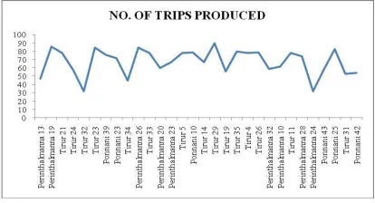
The dependent variables (y) would be the number of trip produced from each of the wards within the divided zones in the selected towns. The data pertaining to the number of trips produced from each of the ward was obtained by conducting the socio-economic survey and forming the O-D matrix.

FIGURE 1. TRIPS PRODUCED

To understand the behavior and factors affecting the travel, one has got the origin of travel when the decision for travel is made. It is where people live as family which is the household. Therefore household data is considered to be the most basic and authentic information about the travel pattern of a city. Ideally one should take the details of all the people in the study to get complete travel details. However, this is not feasible due to large requirement of time and resources needed. In addition this will cause difficulties in handling these large data in modeling stage. Higher sample size is required for large population size, and vice-versa. Normally minimum ten percent samples are required for population less than 50,000. The socio-economic survey for the thesis work was carried out by using the sampling technique, as it is not possible to take into account the entire households within the town. Thus a sampling of 10% was taken to conduct the socio-economic survey. From the socio-economic survey, the origin destination details of each ward within the zones were obtained and these trip details were used to form the O-D matrix. The Fig 1 shows the number of trips produced from each of the selected wards within the three selected towns.

4.2 Independent Variables

Independent or explanatory variables are key input factors that influence the number of trips produced from the wards of a town. The identified independent variables are listed below:

i.Income

ii.Automobile availability

iii.Dwelling type

iv.Average household size

v.Age

vi.Gender

vii.Students

viii.Persons employed

ix.Marital status

part and for the 20 wards that was used for the model validation part.

5. STATISTICAL ANALYSIS OF DATA

5.1 Model Formulation

In this paper, 30 wards along with its identified independent variables were selected for the model formulation. Correlation and regression analysis was performed using Microsoft excel for model formulation.

5.2 Correlation of Variables: Correlation and regressionanalysis are related in the sense that both deal

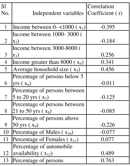
with relationships among variables. The correlation coefficient is a measure of linear association between two variables. Values of the correlation coefficient are always between -1 and +1. A correlation coefficient of +1 indicates that two variables are perfectly related in a positive linear sense; a correlation coefficient of -1 indicates that two variables are perfectly related in a negative linear sense, and a correlation coefficient of 0 indicates that there is no linear relationship between the two variables. The table 1 depict the correlation between each of the independent variables with the dependent variable (trips

produced). It is seen from the table 1that the variables x1, x4, x5, x12, x13, x14, x17, and x18 are moderately

correlated with the trip produced. Among the moderately correlated variables, the independent variables

x1 and x18 are negatively correlated and x4, x5, x12, x13, x14, and x17 are positively correlated with the

depended variable y. Taking into account the collinearity coefficient of the dependent variable with the independent variable and also the presence of multicollinearity, eight explanatory variables were selected. Only the significant and moderately correlated explanatory variables were selected for the model formulation.

TABLE 1. CORRELATION COEFFICIENTS

Sl

No. Independent variables

Correlation Coefficient ( r)

1 Income between 0- <1000 ( x1) -0.395

2

Income between 1000- 3000 (

x2) -0.184

3

Income between 3000-8000 (

x3) 0.256

4 Income greater than 8000 ( x4) 0.341

5 Average household size ( x5) 0.456

6

Percentage of persons below 5

yrs ( x6) -0.011

7

Percentage of persons between

5 to 20 yrs ( x7) -0.125

8

Percentage of persons between

21 to 50 yrs ( x8) -0.085

9

Percentage of persons above

50 yrs ( x9) -0.226

10 Percentage of Males ( x10) -0.077

11 Percentage of Females ( x11) 0.077

12

Percentage of automobile

availability ( x12) 0.489

employed ( x13)

14 Percentage of students ( x14) 0.718

15

Percentage of married people (

x15) 0.194

16

Percentage of single persons (

x16) -0.213

17

Percentage of pucca type of

dwelling ( x17) 0.548

18

Percentage of medium type of

dwelling ( x18) -0.55

The selected explanatory variables are listed below:

•Income between 0- <1000 (x1)

•Income greater than 8000 (x4)

•Average household size (x5)

•Percentage of automobile availability (x12)

•Percentage of persons employed (x13)

•Percentage of students (x14)

•Percentage of pucca type of dwelling (x17)

•Percentage of medium type of dwelling (x18)

Developing the multiple regression equations: Thestatistical technique employed for finding the best

regression estimates was the backward elimination method. The multiple linear regression analysis of the independent variables were performed using the Microsoft excel. Using this tool, different combinations of the independent variables were regressed to find out the most accurate and suitable regression model.

The regression model having highest R, R2 and Adjusted R2 value, minimum standard error of estimate,

low significance F value and low p value for the coefficients of independent variables and y intercept was selected as the best model using the regression analysis. The regression model consisting of the four explanatory variables that is percentage of automobile availability, percentage of persons employed, percentage of students and percentage of pucca type of dwelling was found as the most suitable regression model.

The predictive equation from the multiple regression model is

y=-28.027 + (0.277 × x12) + (1.592 × x13) + (1.447 × x14)+(0.179 × x17) (1)

Where,

y = Trips produced from the residential areas in the medium sized towns on Kerala

x12= Percentage of automobile availability x13= Percentage of persons employed

x14 = Percentage of students

x17 = Percentage of pucca type of dwelling

The first term in the prediction equation (-28.027) is a constant that represents the predicted criterion value when the predictors equal zero. The values of 0.277, 1.592, 1.447 and 0.179 represent regression weights or regression coefficients.

Trip (y) will increase on an average by 0.277, 1.592, 1.447 and 0.179 trips per day for each 1% increase in the Percentage of automobile availability, Percentage of persons employed, Percentage of students and Percentage of pucca type of dwelling respectively.

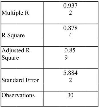
observed value the predicted value of the criterion variable. For this model it has a correlation of 0.9372. This shows that there is a high correlation between the observed and predicted value.

The coefficient of determination is the square of the correlation coefficient (R2). The R-squared of the

regression is the fraction of the variation in the dependent variable that is accounted for (or predicted) by

the independent variables. The obtained coefficient of determination (R2) value is 0.8784, which denotes

that 87.84% of the trip produced is influenced by the variation in the percentage of automobile availability, percentage of persons employed, percentage of students and by the percentage of pucca type of dwelling while 12.16% is explained by other factors.

Adjusted R Square value takes into account the number of variables in the model and the number of observations our model is based on. Adjusted R Square value gives the most useful measure of the

success of the model. The obtained adjusted R2 value is 0.8590, which means that 85.9% of the trip

produced are influenced by the percentage of automobile availability, percentage of persons employed, percentage of students and by the percentage of pucca type of dwelling and these are the independent variable that affect the trips produced to the greatest extend or is the most significant variable when compared to the rest.

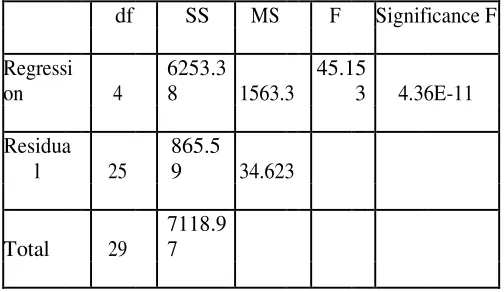
The standard error of the model, is the standard deviation of residuals, indicates the degree of variation on the data about the regression line established. The standard error of the regression model is 5.8842. This means that, the expected error for trip production predicted is off by 5.8842 trips. The error was a comparatively small when the sample size was considered. From the Table 3 the Significance of F value indicates the probability that the Regression output could have been obtained by chance.

A small Significance of F confirms the validity of the Regression output. Since the obtained significance of F value was 4.36139E-11, it means that there was only a 4.36139E-09 % chance that the regression output was merely a chance occurrence. Thus increasing the overall accuracy and significance of the formulated model. The p-value is a percentage and it tells you how likely it is that the coefficient for that independent variable emerged by chance and does not describe a real

TABLE 2. REGRESION STATISTICS

Multiple R

0.937

2

R Square

0.878

4

Adjusted R

Square

0.85

9

Standard Error

5.884

2

Observations 30

TABLE 3. ANOVA TEST RESULTS

df SS MS F Significance F

Regressi

on 4

6253.3

8 1563.3

45.15

3 4.36E-11

Residua

l 25

865.5

9 34.623

Total 29

7118.9

7

TABLE 4. REGRESSION COEFFICIENTS

Coefficien ts Standard Error t

Stat p-value Lower 95% Upper 95% Intercept

-28.027 7.525 -3.725

0.00

1 -43.524 -12.529

x

12 0.277 0.08 3.44

0.00

2 0.111 0.442

x

13 1.592 0.259 6.136 2.10E-06 1.058 2.127

x

14 1.447 0.401 3.61

0.00

1 0.622 2.272

x

17 0.179 0.057 3.135

0.00

4 0.061 0.296

relationship. A p-value of 0.05 means that there is a 5% chance that the relationship emerged randomly and a 95% chance that the relationship is real. It is generally accepted practice to consider variables with a p-value of less than 0.1 as significant, though the only basis for this cutoff is convention. The lower the Value, the higher the likelihood that that coefficient or Y-Intercept is valid. From the Table 4 the p-value for the coefficient of percentage of automobile availability, percentage of persons employed percentage of students and percentage of pucca type of dwelling was 0.001, 0.002, 0.0000021, 0.001 and 0.004 respectively. This indicates that there was only a minor chance that the result occurred by chance. Hence the accuracy of the model increases to a greater percentage.

Model Validation

Model validation is an important step in the modeling process and helps in assessing the reliability of models before they can be used in decision making. For the model validation, the testing set comprising of 20 wards was used. These set of data are new data which are different from the data taken for model formulation.

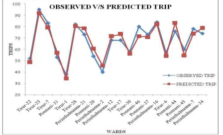
Graphical diagnosis of model validation: Plotting ofdiagnostic graph is a technique used to validate

almost coincide with each other. This graph indicated the strong validity of the regression model and that the predicted trips were almost accurate.

FIGURE 2. OBSERVED v/s PREDICTED TRIPS

REFERENCES

[1] Olugbenga Joseph and Oluyemisi Opeyemi, “Regression Model of Household Trip Generation of Ado-Ekiti Township in Nigeria,” European Journal of Scientific Research, ISSN 1450-216X Vol.28 , no.1, EuroJournals Publishing, Inc. 2009, , pp.132-140.

[2] William J. Fogarty, “Trip Production Forecasting Models for Urban Areas,” Transportation Engineering Journal © ASCE, Vol. 102, No. 4, November 1976, pp. 831-845.

[3] Michael G. McNally, “The Four Step Model,” Institute of Transportation Studies University of California, 2007.

[4] Kevin B. Modi, L. B. Zala, T. A. Desai, and F. S. Umrigar, “Transportation Planning Models,” National Conference on Recent Trends in Engineering & Technology, May 2011.

[5] Charles L. Purvis, Miguel Iglesias, and Victoria A. Eisen, “Incorporating Work Trip Accessibility in Non-Work Trip Generation Models in the San Francisco Bay Area,” Paper submitted to the Transportation Research Board for presentation at the 75th Annual Meeting, January 1996.

[6] Nonito M. Magdayojr, “Study on the Application of Trip Generation Analysis for Residential Condominium Developments in Metro

Manila,” Final Paper, Undergraduate Research Program in Civil Engineering, march 2008

[7] John S. Miller, P.E.Lester A. Hoel, P.E. Arkopal K. Goswami, and Jared M. Ulmer, “Borrowing Residential Trip Generation Rates,” Journal of Tansportation Engineering © ASCE, February 2006, pp. 105-113.

[8] Papacostas C.S. and Prevedouros P.D., Transportation Engineering and Planning,” SI Edition, Prentice-Hall Inc Singapore, 2005. [9] Abdul Khalik Al-Taei and Amal M. Taher, “Prediction Analysis of Trip Production Using Cross-Classification Technique,” Al

-Rafidain Engineering, vol.14, no.4, 2006.

[10] Matthew Femal, “Improving Trip Generation Equations,” Thesis report, School of Engineering and Applied Science, University of Virginia, 2010.

[11] MichaelAnderson and Justin P. Olander,“Evaluation of Two Trip Generation Techniques for Small Area Travel Models,” Journal of