Maximum likelihood estimation for directional conditionally autoregressive models

Maximum Likelihood Estimation for

Directional Conditionally Autoregressive

Models

Minjung Kyung

and Sujit K. Ghosh

Institute of Statistics Mimeo Series #2597

Abstract

A spatial process observed over a lattice or a set of irregular regions is

usu-ally modeled using a conditionusu-ally autoregressive (CAR) model. The

neighbor-hoods within a CAR model are generally formed using only the inter-distances

between the regions. To accommodate the effect of directions, a new class of

spatial models is developed using different weights given to neighbors in

dif-ferent directions. The proposed model generalizes the usual CAR model by

accounting for spatial anisotropy. Maximum likelihood estimators are derived

and shown to be consistent under some regularity conditions. Simulation

stud-ies are presented to evaluate the finite sample performance of the new model

as compared to CAR model. Finally the method is illustrated using a data set

on the crime rates of Columbus, OH.

Key words: Anisotropy; Condionally autoregressive models; Lattice data, Max-imum likelihood estimation, Spatial analysis.

∗_{Minjung Kyung is a graduate student and Sujit K. Ghosh is an associate professor, both at the}

1

Introduction

In many studies, counts or averages over arbitrary regions, known as lattice or area

data (Cressie, 1993), are observed and spatial analysis is performed. Given a set of

geographical regions, observations collected over regions nearer to each other tend to

have similar characteristics as compared to distant regions. In geoscience, this feature

is known as the Tobler’s first law (Miller, 2004). From a statistical perspective, this

feature is attributed to the fact that the autocorrelation between the observations

collected from nearer regions tends to be higher than those that are distant.

In general, given a set of regionsS₁, . . . , S_n, we consider a generalized linear model

for the aggregated responses, Y_i =Y(S_i), as

E[Y_i|Z_i] = g(Z_i)

and Z_i = μ_i+η_i i= 1,2, . . . , n, (1)

where g(·) is a suitable link function, μ_i’s denote large-scale variations and η_i’s

rep-resent small-scale variations (or spatial random effects). The latent spatial process

Z_i’s are usually modeled using a conditionally autoregressive (CAR) model (Besag,

1974) or a simultaneously autoregressive (SAR) model (Ord, 1975). These models

have been widely used in spatial statistics (Cliff and Ord, 1981). The CAR and SAR

models are used to study how a particular region is influenced by its “neighboring

regions”. The large sacle variations, μ_i’s are ususally modeled as a function of some

predictor variables (e.g., latitudes, longitudes and other areal level covariates) using

a parametric or semiparametric regression model (see van der Linde et al., 1995).

In this article, we instead focus on developing more flexible models for the spatial

random effects η_i’s.

effects models to explain the latent spatial process using suitably formed neighbors

(Breslow and Clayton, 1993). Gaussian CAR process has the merit that the finite

dimensional joint distributions of the spatial process are multivariate Gaussian

dis-tributions. So, the maximum likelihood (ML) and the Bayesian estimates are easily

obtained. Howver one of the major limitations of the CAR model is that the

neigh-bors are formed using some form a distance metric and the effect of the direction

is completely ignored. However, if the underlying spatial process is anisotropic, the

magnitude of autocorrelation between the neighbors might be different in different

directions. This limitation serves as our main motivation and an extension of the

regular CAR process is proposed that can capture anisotropy. The newly proposed

spatial process will be termed as the directional CAR (DCAR) model. In Section 2,

we define the new spatial process and present statistical inferences for the

parame-ters based on maximum likelihood (ML) theory. In Section 2.2, the ML estimator is

shown to be consistent under some regularity conditions. Section 3 presents the finite

sample performance of the ML estimators and the newly proposed DCAR models are

compared against the regular CAR models in terms of popular information theoretic

criteria. In Section 4, the proposed method is illustrated and compared with regular

CAR using a data set of the crime rates in Columbus, OH. Finally, in Section 5, some

extensions of the DCAR model are discussed.

2

Directional CAR models

Consider again the model described by (1). In this section, we develop a new model

for the Z_i’s. For illustrations and notation simplicity assume that S_i are regions in a

S_i S_j

alpha(S_i,S_j)

Figure 1: The angle (in radian) α_ij

inference presented in this article can easily be extended to higher dimensional data.

Let s_i = (s_1i, s_2i) be a centroid of the sub-region S_i, where s_1i corresponds to the

horizontal coordinate (x-coordinate) and s_2i corresponds to the vertical coordinate

(y-coordinate). The angle (in radian) between s_i and s_j is defined as

α_ij =α(S_i, S_j) =

⎧ ⎨ ⎩

tan−1(s2_s1j−s2i

j−s1i) if s2j−s2i ≥0

−π−tan−1(s2_s1j−s2i

j−s1i) if s2j−s2i <0

for all j =i. We consider directions of neighbors from the centroid of subregion S_i’s.

For example, in Figure 1, S_j is in the north-east region of S_i and hence α(S_i, S_j) is

in [0,π₂). Let N_i represents a set of indexes of neighborhoods for the i-th region S_i

that are based on some form distance metric (say as in a regular CAR model). We

can now create new sub-regions, for each i, as follows:

Ni1 = {j :j ∈ Ni,0≤αij < π

2},

Ni2 = {j :j ∈ Ni,

π

2 ≤αij < π},

Ni3 = {j :j ∈ Ni, π ≤αij <

3 2π},

Ni4 = {j :j ∈ Ni,3

2π≤αij <2π}.

However, these directional neighborhoods should be chosen carefully so that for each

a single site or else in which every site is a neighbor of every other site in the set

(Besag, 1974).

This would allow us to show the existence of the spatial process by using the

Hammersley-Clifford Theorem (Besag, 1974 p.197-198) and to derive the finite

di-mensional joint distribution of process using only a set of full conditional

distribu-tions. For instance, if j ∈ N_i1 then we should ensure that i ∈ N_j3. For the above

set of four sub-neighborhoods, we can combine each pair of the diagonally opposite

neighborhoods to form a new neighborhood, i.e., we can create N_i∗₁ =N_i1N_i3, and

N∗

i2 =Ni2Ni4 fori= 1, . . . , n. Now it is easy to check that ifj ∈ Ni∗1, theni∈ Nj∗1.

Thus, we redefine two subsets of N_i’s as follows:

N∗

i1 = {j :j ∈ Ni and (0≤αij < π₂ orπ ≤αij < 3₂π)}

N∗

i2 = {j :j ∈ Ni and (π₂ ≤αij < π or 3₂π ≤αij <2π)}. (2)

Then, each ofN_i∗₁ andN_i∗₂ forms a clique and thatN_i =N_i∗₁N_i∗₂. The above scheme

of creating new neighborhoods based on the inter-angles,α_ij’s can be extended beyond

just two sub-neighborhoods so that each of the new sub-neighborhood forms a clique.

But for the rest of the article we restrict our attention to case with only two

sub-neighborhoods as described in (2).

Based on subsets of the associated neighborhoods,N_i∗₁ and N_i∗₂, we can construct

directional weight matrices W(1) = ((w(1)_ij )) and W(2) = ((w(2)_ij )), respectively. For

instance, we can define the directional proximity matrices as w(1)_ij = 1 ifj ∈ N_i∗₁ and

w(2)_ij = 1 if j ∈ N_i∗₂. Notice that W = W(1)+W(2) reproduces the commonly used

proximity matrix based on distances as in a regular CAR model.

In order to model the large-scale variations, without loss of any generality we

and β= (β₁, . . . , β_q)T is a vector of regression coefficients. Notice that nonlinear

re-gression functions involving smoothing splines and polynomials can be re-written in

the above canonical form (e.g., see Wahba, 1977). From model (1) it follows that

E[Z] =Xβ and Var[Z] =Σ(ω), (3)

where ω denotes the vector of spatial autocorrelation parameters and other variance

components. Notice that along with (3) the model (1) can be used for discrete

responses using a generalized linear model framework (Schabenberger and Gotway,

2005, p.353). We now develop a model for Σ(ω) that accounts for anisotropy.

Let δ₁ and δ₂ denote the directional spatial effects corresponding to N_i1’s and

Ni2’s, respectively. We define the distribution of Zi conditional on the rest of Zj’s for

j =i using only the first two moments:

E[Z_i|Z_j =z_jj =i,x_i] = xT_i β+

2

k=1

δ_k

n

j=1

w_ij(k)z_j−xT_jβ

Var[Z_i|Z_j =z_jj =i,x_i] = σ

2

m_i, (4)

where w(_ijk) ≥0 andw(_iik) = 0 for k = 1,2 and m_i =n_j=1w_ij.

The joint distribution based on a given set of full conditional distributions can be

derived using the Brook’s Lemma(Brook, 1964), provided the positivity condition is

satisfied. For the DCAR model, by construction it follows that each of N_i∗₁ and N_i∗₂

defined in (2) forms a clique for i= 1, . . . , n. Thus, it follows from the

Hammersley-Clifford Theorem that the latent spatial process Z_i of a DCAR model exists and is a

Markov Random Field (MRF). We now derive the exact joint distribution of theZ_i’s

2.1

Gaussian DCAR models

The Gaussian CAR model has been used widely for the latent spatial process Z_i.

In this section, we study merits of the Gaussian DCAR model. As we discussed in

previous section, the joint distribution can be easily derived from the conditional

distributions by using Brook’s Lemma.

Assume that the full conditional distributions ofZ_i’s are given as

Z_i|Z_j =z_j, j =i,x_i ∼N

xT_i β+

2

k=1

δ_k

n

j=1

w(_ijk)z_j −xT_jβ, σ

2

m_i

, (5)

where w(_ijk) for k = 1,2 are the directional weights. It can be shown that this latent

spatial DCAR process Z_i’s is a MRF. Thus, by Brook’s lemma and the

Hammersley-Clifford Theorem, it follows that the finite dimensional joint distribution is a

multi-variate Gaussian distribution given by

Z ∼N_nXβ, σ2(I−δ₁W(1)−δ₂W(2))−1D, (6)

where Z = (Z₁, . . . , Z_n)T and D = diag(_m11 , . . . , _m1

n). For simplicity, we denote the

variance-covariance matrix of DCAR process by Σ∗_Z ≡σ2(I−δ₁W(1)−δ₂W(2))−1D.

For a proper Gaussian model, the variance-covariance matrixΣ∗_Z is required to be

positive definite. If we use the standardized directional proximity matrices ˜W(k) =

(( ˜w_ij(k) = w

(k)

ij

mi )),k = 1,2, it can be easily shown that Σ

∗

Z is symmetric.

Next, we derive a sufficient condition that ensures that the variance-covariance

matrix Σ∗_Z is non-singular. As D is a diagonal matrix, we only require suitable

conditions on ˜W(k) and onδ_k fork = 1,2. The following results provides a sufficient

condition:

symmetric matrix with non-negative entries, diagonal 0 and each row sums to unity. If max_1≤k≤K|δ_k|<1, then the matrix A is positive definite.

Proof: Let a_ij denote the (i, j)-th element of A. Notice that for each i = 1,2. . . , n, we have

j=i

|a_ij|=

j=i

|

K

k=1

δ_kw_ij(k)| ≤

K

k=1

|δ_k|

j=i

w(_ijk) <

K

k=1 j=i

w(_ijk) = 1 =a_ii

Hence it follows from Lemma 2 (see Appendix A) that A is positive definite.

Notice that when δ₁ = δ₂ = ρ, DCAR(δ₁, δ₂, σ2) reduces to CAR(ρ, σ2). The

next step of a statistical analysis is to estimate unknown parameters of the DCAR

model based on the observed responses and the explanatory variables and to predict

future values at unobserved sites. Thus, in the next section, we discuss the maximum

likelihood (ML) methods for the spatial autoregressive models.

2.2

Parameter estimation using ML theory

With Gaussian DCAR model of the latent spatial process Z_i’s, we describe how to

estimate parameters and associated measures of uncertainties based on ML methods.

Mardia and Marshall (1984) have given sufficient conditions in the case of

Gaus-sian process for the consistency and asymptotic normality of the ML estimators.

Based on their results, first we describe the numerical computation of the MLE of

η = (βT, σ2,δT)T, where δ = (δ₁, δ₂)T, for a Gaussian DCAR model of Z_i’s. Then,

we show that the ML estimator of Gaussian DCAR model is consistent and

asymp-totically normal.

In the case of autoregressive models, likelihood is a complex nonlinear function of

is a complex nonlinear function of δ₁ and δ₂ which appear in the variance-covariance

matrix. Here, for the latent spatial DCAR process Z_i’s, under the joint multivariate

Gaussian distribution, the log-likelihood function is given by

(β, σ2,δ) = −n

2ln(2πσ

2₎₋ 1

2ln|A

∗_(δ)−1_D|

− 1

2σ2(Z−Xβ)

T_D−1_A∗_{(δ)(Z−Xβ) (7)}

where A∗(δ) =I−δ₁W˜ (1)−δ₂W˜ (2) and D = diag(_m11 , . . . ,_m1

n). Thus, for known δ,

the profile ML estimators of β and σ2 are given by

β(δ) = XTD−1A∗(δ)X−1XTD−1A∗(δ)Z

σ2(δ) = n−1(Z−Xβ(δ))TD−1A∗(δ)(Z−Xβ(δ)).

Substituting back into (7), the ML estimator ofδ can be obtained by maximizing the

profile log likelihood,

∗_{(δ) = −}n

2 ln(σ2(δ)) + 1

2ln|A

∗_{(δ)| (8)}

which can be numerically maximized to obtain δ₁ and δ₂.

In order to maintain the restriction max(|δ₁|,|δ₂|) < 1, we use the

“L-BFGS-B” method (Byrd, et al., 1995) to compute the ML estimates maximizing the

log-likelihood. We also extract the Hessian matrix to estimate the information matrix.

In other words, we use observed Fisher information matrix to obtain the standard

errors (s.e.’s) of η. It has been shown by Efron and Hinkley (1978) that use of the

observed Fisher information matrix results into more efficient estimator than the use

of the expected Fisher information matrix.

For large samples, the sampling distribution of the MLE will be shown to have

variance determined by the Fisher information. To derive the Fisher information

matrix of MLE’s for Gaussian DCAR model, the steps of p. 483-484 in Section 7.3.1

of Cressie (1993) are followed. However, for the derivatives of the variance-covariance

matrix, Lemma 3 and Lemma 4 in Appendix A are used. For a DCAR model, we

define a vector of variance-covariance parameters as γ = (σ2,δT)T = (γ₁ =σ2, γ₂ =

δ₁, γ₃ =δ₂)T. Then, we denoteΣ_(i) =∂Σ/∂γ_i andΣ(i) =∂Σ−1/∂γ_i =−Σ−1Σ_(i)Σ−1

for i= 1,2,3. Also, Σ_(ij) =∂2Σ/∂γ_i∂γ_j and Σ(ij) = ∂2Σ−1/∂γ_i∂γ_j for i, j = 1,2,3. Thus, for a DCAR model,

ΣΣ(1) =−(σ−2)I_n×n, ΣΣ(2) =−A∗(δ)−1W˜ (1) and ΣΣ(3) =−A∗(δ)−1W˜(2).

Therefore, the Fisher information matrix for Gaussian DCAR model has the form

I(η) =

⎡ ⎢ ⎢ ⎢ ⎢ ⎢ ⎢ ⎢ ⎣

σ−2XTD−1/2A∗(δ)D−1/2X 0 0 0 0T n₂σ−4 1₂σ−2tr(G₁) 1₂σ−2tr(G₂)

0T 1₂σ−2tr(G₁) 1₂ν₁ 1₂tr(G₁G₂)

0T 1₂σ−2tr(G₂) 1₂tr(G₁G₂) 1₂ν₂

⎤ ⎥ ⎥ ⎥ ⎥ ⎥ ⎥ ⎥ ⎦

,

(9)

where G_k = ˜W(k)A∗(δ)−1, ν_k =tr(G_kG_k) =tr(G2_k), for k = 1,2. We estimate this

Fisher information (FI) matrix (9) to obtain the asymptotic variances of parameters

using the observed FI.

BecauseZ is a single observation fromN_n(Xβ,Σ=Σ_Z), it is not obvious thatη

is consistent and asymptotically normal. Sweeting (1980) has given a general result of

weak consistency and uniform asymptotic normality for MLE’s based on dependent

observations. Using Sweeting’s result, Mardia and Marshall (1984) prove the following

theorem.

p×1vector of unknown large-scale parameters andΣ is function ofγ, a k×1 vector of unknown small-scale (spatial) parameters. Let λ₁ ≤ · · · ≤λ_n be the eigenvalues of

Σ and let those of Σ_(i) and Σ_(ij) be {λi_l : l = 1, . . . , n} and {λij_l : l = 1, . . . , n}, with

|λi₁| ≤ · · · ≤ |λi_n| and |λ₁ij| ≤ · · · ≤ |λij_n| for i, j = 1, . . . , k. Suppose that, as n → ∞,

(i) limλ_n=C <∞, lim|λi_n|=C_i <∞, lim|λij_n|=C_ij <∞ for all i, j = 1, . . . , k

(ii) ||Σ_(i)||−2 = O(n−21−α), for some α > 0 for i = 1, . . . , k (||G|| denotes the Euclidean matrix norm, (_i,jg2_ij)1/2 ={tr(GTG)}1/2)

(iii) for alli, j = 1, . . . , k, a_ij = lim{t_ij/(t_iit_jj)12}exists, wheret_ij =tr(Σ−1Σ_(i)Σ−1Σ_(j))

and A= ((a_ij)) is a nonsingular matrix

(iv) lim(XTX)−1 = 0.

Then these conditions are sufficient for the asymptotic normality and weak consistency

ofη; that isη∼N(η,I(η)), whereI(η)is the information matrix andη = (βT,γT)T.

For a proof see the paper of Mardia and Marshall (1984).

We show that the above sufficient conditions are satisfied by the MLE of the

DCAR model under some additional regularity conditions and hence we establish the

asymptotic normality and weak consistency of η under DCAR model.

Theorem 2 The conditions stated in Theorem 1 are satisfied by the DCAR model if

0 < lim infm₍₁₎ ≤ lim supm_(n) <∞ as n → ∞ where m_i is number of neighbors of

subregion S_i, m₍₁₎ = min(m₁, . . . , m_n) and m_(n)= max(m₁, . . . , m_n).

The proof of the Theorem 2 is given in Appendix B.

In order to study the finite sample performance of ML estimators, we conduct

a simulation study. In this simulation study, we focus on the behavior of Gaussian

2.3

A simulation study

Mardia and Marshall (1984) conducted a simulation study with 10×10 unit spacing

lattice, based on samples generated from normal distribution with mean zero and a

spherical covariance model. The sampling distribution of the MLE’s of the parameters

were studied based on 300 Monte Carlo samples. Following a similar setup, for our

simulation study, we selected an 15×15 unit spacing lattice and generated 500 samples

(N=500)Z_i’s from a multivariate normal distribution with meanXβand the

variance-covariance σ2A∗(δ)−1D, where A∗(δ) = I−δ₁W˜ (1) −δ₂W˜ (2). The X matrix was

chosen to represent the lattice nad longitude coordinates in addition to an intercept.

The true value of the parameters were fixed at β = (1,−1,2)T and σ2 = 2. For the

above mentioned DCAR model, to study the sampling distributions of MLE’s δ₁ and

δ₂, we consider four different sets of δ’s:

Case 1: δ₁ =−0.95 & δ₂ =−0.97: negative boundary points

Case 2: δ₁ =−0.30 & δ₂ = 0.95: negative point and positive boundary point

Case 3: δ₁ =−0.95 & δ₂ = 0.97: negative boundary point and positive boundary point

Case 4: δ₁ = 0.95 & δ₂ = 0.93: positive boundary points.

It is expected that for the values of the parameters near the boundary of the parameter

space, there might be unexpected behaviors of the MLE’s.

As we discussed in Section 2.2, in order to maintain the restriction max(|δ₁|,|δ₂|)<

1, we use the “L-BFGS-B” method to compute the ML estimates within the _optim

function of the software _R to maximize the log-likelihood. To obtain the standard

errors (s.e.’s) of η, it is also computationally easier to directly obtain the Hessian

matrix from the output of the _optim function.

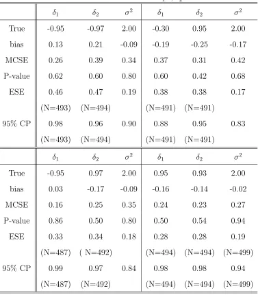
First, from the Table 1, notice that there are few missing estimates of the estimated

standard errors (ESE) based on the observed Fisher information matrix. This is due

to the fact that _R has a function _deriv that numerically computes the derivative of

complicated expressions which can lead to numerical instabilities. We observe that

for all the four choices of δ, there are no significant biases (all p-values are bigger

than 0.42). Furthermore, it appears that the estimated standard errors (ESE’s) of

δ₁ and δ₂ are good approximations to finite sample Monte Carlo standard errors

(MCSE’s) when the true values are positive. For all these boundary values of δ, the

nominal 95% coverage probability (CP) is relatively away from 0.95 indicating that

the MLE tends to estimate the true value with higher uncertainty when all δ₁ andδ₂

are near the boundary. The high coverage probability of MLE based on a symmetric

confidence interval may be due to the skewness of the sampling distribution that we

have observed in our empirical studies. It was observed that the estimates appear to

be skewed to right for the negative extreme value and they are skewed to the left for

the positive extreme value.

For the results of ML estimation of σ2 of DCAR model, the bias of σ2 tends to

be slightly negative. In other words, the MLE’s of σ2 tend to underestimate the true

values. However, it is to be noted that these biases are not statistically significant

(all four p-values are greater than 0.6). Thus, for all cases, MLE of σ2 is reasonable

estimate.

For the estimation ofβ’s, we observe that the finite sample performance of MLE’s

of β’s of DCAR model are close to the large sample Gaussian approximation. Also,

biases are not significant and nominal coverage probabilities were all found to be close

Table 1: Performance of MLE’s of δ₁’s, δ₂’s and σ2’s

δ₁ δ₂ σ2 δ₁ δ₂ σ2

True -0.95 -0.97 2.00 -0.30 0.95 2.00

bias 0.13 0.21 -0.09 -0.19 -0.25 -0.17

MCSE 0.26 0.39 0.34 0.37 0.31 0.42

P-value 0.62 0.60 0.80 0.60 0.42 0.68

ESE 0.46 0.47 0.19 0.38 0.38 0.17

(N=493) (N=494) (N=491) (N=491)

95% CP 0.98 0.96 0.90 0.88 0.95 0.83

(N=493) (N=494) (N=491) (N=491)

δ₁ δ₂ σ2 δ₁ δ₂ σ2

True -0.95 0.97 2.00 0.95 0.93 2.00

bias 0.03 -0.17 -0.09 -0.16 -0.14 -0.02

MCSE 0.16 0.25 0.35 0.24 0.23 0.27

P-value 0.86 0.50 0.80 0.50 0.54 0.94

ESE 0.33 0.34 0.18 0.28 0.28 0.19

(N=487) ( N=492) (N=494) (N=494) (N=499)

95% CP 0.99 0.97 0.84 0.98 0.98 0.94

3

Model comparison using information criteria

The DCAR model is a generalization of the CAR model. So it would be interesting

to investigate what happens when someone fits a CAR model to a data set generated

under a DCAR model and vice versa. To compare models, we consider the Akaike’s

Information Criterion (AIC) (Akaike, 1974) and the Bayesian Information Criterion

(BIC) (Schwartz, 1978) based on the ML method. AIC, a penalized-log-likelihood

criterion, is defined by

AIC =−2 (η) + 2k,

where (η) is defined in (7) andk is number of parameters. Also, BIC is defined by

BIC =−2 (η) +kln(n),

wherenis the number of observations. In theory, we select the model with the smaller

AIC and BIC values. We consider two cases based on data generated from a (i) CAR

model and (ii) DCAR model.

3.1

Results based on CAR data

With samples from Gaussian CAR process, we fit both CAR and DCAR models,

respectively. Notice that if there is no directional difference in the observed spatial

data, then the estimates of δ₁ should be very similar to the estimates of δ₂. Thus

we might expect very similar estimates for δ₁ and δ₂ based on a sample from CAR

process because CAR(ρ, σ2) = DCAR(ρ, ρ, σ2). To study the sampling distribution

of ρ, we consider five different values of ρ’s, Case 1:ρ = −0.95, Case 2:ρ = −0.25,

Case 3:ρ = 0, Case 4:ρ = 0.25 and Case 5:ρ = 0.95. For each case, we compare the

From the results based on the ML estimates of CAR model, we observe that for

all the cases there are no significant biases at 5% level. The ESE of ρ is a good

approximation to finite sample variance when the spatial dependence is weak such

as in cases 2,3, and 4, because the ESE’s are close to MCSE’s. However, when the

true value is near negative boundary, MLE tends to estimate the true value with high

uncertainty. For all cases, the biases of MLE’s of σ2 tend to be slightly negative.

However, these negative biases are not significant (all p-values are bigger than 0.7).

For the estimation ofβ’s, the estimates did not have any significant bias (all p-values

are bigger than 0.9). We have presented these results due to lack of space but are

available in the first author’s doctoral thesis.

3.1.1 Estimation under model misspecification

From the results of the ML estimates of DCAR model, we observe that the ML

estimates ofδ andσ2 are slightly negatively biased for all cases except when the true

value of ρ is near negative boundary, ρ = −0.95. However, based on p-value, we

conclude that there is no significant bias (all p-values are bigger than 0.5). We notice

that the ML estimates of δ and σ2 of DCAR model are similar to the estimates ofρ

and σ2 of CAR model, respectively. It means that with data sets from a CAR model,

the sampling distributions of parameters are quite similar for either fitting CAR or

DCAR model. However, the estimates of δ for each cases have larger MCSE and

ESE values than the estimates of ρ as expected. The estimates ofβ based on DCAR

model is not affected at all even if the data was generated from a CAR model. This

is also expected as under both models Xβ is the mean ofy.

Instead of comparing the parameter estimates of CAR and DCAR models based

Table 2: Compariosn of AIC and BIC between CAR and DCAR models with data sets from CAR process (PCD = Percentage of Correct Decision)

DGP CAR(ρ=−0.95) CAR(ρ=−0.25) CAR(ρ= 0.00)

Fit CAR DCAR CAR DCAR CAR DCAR

PCD(AIC) 90% 10% 81% 19% 88% 12%

P-value 0.01 0.94 0.92

PCD(BIC) 95% 5% 94% 6% 95% 5%

P-value 0.01 0.93 0.91

DGP CAR(ρ= 0.25) CAR(ρ= 0.95)

Fit CAR DCAR CAR DCAR

PCD(AIC) 84% 16% 95% 5%

P-value 0.63 0.51

PCD(BIC) 96% 4% 98% 2%

P-value 0.61 0.51

performance. It has been shown by Stone (1977) that the use of AIC is similar to

cross-validation. We define DGP as the data generating process and FIT as the data

fitting models. Also, we define PDC as the percentage of correct decision. From Table

2, we observe that AIC and BIC of CAR model are smaller than those of DCAR model

for the same data sets from CAR process for all five cases. PCD based on calculated

AIC values is 90% for samples from CAR process when the true ρ=−0.95. It means

that for N = 500 samples from CAR process withρ=−0.95, if we fit both CAR and

DCAR models, 90% of AIC’s of CAR models is smaller than those of DCAR models.

However, p-values for hypothesis that AIC or BIC values of CAR model is the same

as that of DCAR model, are much larger than 0.05 for Cases 2,3,4 and 5, but for Case

1, p-values for hypothesis test are less than 0.05. In other words when the true value

of ρ is near negative boundary (ρ = −0.95), for the data set of CAR process, CAR

model fits better than DCAR model. Other cases, we can use either CAR or DCAR

model for the ML method based on samples from CAR process. This is expected as

Based on the performance of AIC and BIC, we observe that for the data set

generated from CAR with ρ = −0.95, the CAR model fits significantly better than

the DCAR model. However, for all other cases that we investigated, we conclude that

we may safely use DCAR model even when the data is generated from a CAR model.

3.2

Results based on DCAR data

In this section, we fit both CAR and DCAR models to the data sets generated from

DCAR model. In this case, there might exist somewhat unexpected sampling

distri-bution of ρ as it will not be able to capture the directional effects.

3.2.1 Estimation under model misspecification

From the ML estimates of ρ, it appears that ρ seems to estimate the mean of the

true values of δ₁ and δ₂ for a sample from a DCAR process. Therefore, we define the

pseudo-true value of ρ as the mean of the true values of δ₁ and δ₂. By fitting DCAR

and CAR model to samples from DCAR process, we observe that if the mean of δ₁

andδ₂ is near positive or negative boundary, the sampling distribution ofρ₀ = δ1b+₂δ2b is

very similar to the sampling distribution ofρ. Estimates ofρ₀’s are slightly negatively

biased except Case 1. However, as p-values are bigger than 0.3, we conclude that

there is no significant biases of all parameters (Results are not tabulated due to lack

of space). For the estimates of σ2, the estimates were found to be slightly negatively

biased if δ₁ and δ₂ were near the same negative or positive boundary. However, if δ₁

and δ₂ are in negative and positive area separately, the estimates of σ2 are slightly

positively biased. Again such biases are not statistically significant because all

p-values are bigger than 0.6. We notices that if the true value ρ₀ = δ1+₂δ2 is near

boundary, the estimates of ρare skewed left.

From the Table 3, we observe that CAR model has smaller AIC values than

DCAR model for samples from DCAR process when δ₁ ≈ δ₂ as expected as CAR is

nested under DCAR. However, when δ₁ and δ₂ are in negative and positive valued,

respectively, PCD of AIC for DCAR model is 70% for Case 2 and 3, respectively, thus

AIC picks up the true model, DCAR model, more frequently. Nevertheless, p-values

for hypothesis that AIC of CAR model is the same as that of DCAR model, are

greater than 0.05 for all cases. From the Table 3, we observe that BIC picks up a

DCAR model more frequently with percentage of correct decisions by 62%, when the

data are from DCAR process with δ₁ = −0.95 and δ₂ = 0.97, two extreme values

in each negative and positive parameter space and by 64% when the data are from

DCAR process with δ₁ =−0.30 andδ₂ = 0.95.

Notice that BIC penalizes the DCAR model in favor of CAR model whenδ₁ ≈δ₂

as expected because a DCAR with δ₁ = δ₂ reduces to a CAR model. In summary,

we would recommend the use of BIC as a good model selection criteria compared to

AIC in choosing the better model when comparing CAR and DCAR model.

Therefore, the CAR model captures the mean of directional spatial effects when

the data is generated from a DCAR model. The use of information criterion suggests

that DCAR model works better if there exist directionally different relationship within

neighbors and there is no significant loss of efficiency even if the data arise from a

Table 3: Compariosn of AIC and BIC between CAR and DCAR models with data sets from DCAR process (PCD = percentage of correct decisions)

DGP DCAR(δ₁ =−0.95, δ₂ =−0.97) DCAR(δ₁ =−0.30, δ₂ = 0.95)

Fit CAR DCAR CAR DCAR

PCD(AIC) 91% 9% 30% 70%

P-value 0.07 0.09

PCD(BIC) 95% 5% 36% 64%

P-value 0.06 0.08

DGP DCAR(δ₁ =−0.95, δ₂ = 0.97) DCAR(δ₁ = 0.95, δ₂ = 0.93)

Fit CAR DCAR CAR DCAR

PCD(AIC) 30% 70% 96% 4%

P-value 0.40 0.17

PCD(BIC) 38% 62% 98% 2%

P-value 0.38 0.17

4

Data analysis

We illustrate the fitting of DCAR and CAR model using a real data set by estimating

the crime distribution in Columbus, Ohio collected in the year of 1980. We also use

in-come level and housing values as predictors for crime rates. These observations were

collected in 49 contiguous Planning Neighborhoods of Columbus, Ohio.

Neighbor-hoods correspond to census tracts, or aggregates of a small number of census tracts.

Original data set can be found in Table 12.1 of Anselin (1988, p.189). In this data

set, the crime variable pertains to the total of residential burglaries and vehicle thefts

per thousand households. The income and housing values are measured in thousands

of dollars. Anselin (1988) illustrated the existence of spatial dependence by using

diagnostic tests based on ordinary least squares (OLS) estimation, ML estimation

using a mixed regressive-autoregressive model and ML estimation using SAR model.

Notably, Anselin considered two sets of separate regression for the east and west side

Lagrange Multiplier statistics, he concluded that when SAR model is used, there

ex-ists structural instability. It means that given a SAR spatial structure, the regression

equation for the east side of the city is different from that of the west. Instead of

using a generalized linear model fro count data, we make a variance stabilizing

log-transformation for Poisson counts and treat the crime rate to be continuous variable.

With log-transformed crime rate, we assume Gaussian distribution with CAR and

DCAR spatial structure.

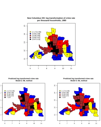
We plot the the log-transformed crime rates that are divided into 5 intervals of

each 20% quantiles in Figure 2. From original data, we observe that Y₄ and Y₁₇ have

extremely small values. The region S₄ is on a boundary in Columbus, OH, but S₁₇

is inside in study region. Also, for log transformed data, we observe that Y₄ and Y₁₇

are possibly outliers because those are smaller than 2.5% quantile of the entire data.

Thus, we eliminate Y₄ and Y₁₇ as outliers. From linear model without considering

spatial dependency, we observe that only house value has a significant effect on the

log-transformed crime rate. However, when Y₄ and Y₁₇ are deleted as outliers, we

observe that only house income has a significant effect based on a linear model. From

the estimated correlogram in Figure 2, it appears that spatial correlations are not as

strong. We model the log-transformed crime rate with income and housing values as

the explanatory variables deleting the outliers.

For this data set, we denoteZ_i = log(Y_i) fori= 1,2, . . . , n, whereY_i is the total of

residential burglaries and vehicle thefts per thousand households of sub-areaiin 1980.

Thus, Z_i is a log transformed crime rate of sub-area S_i. Also, we denote X₁ as the

centered housing value in thousand dollars andX₂ as the centered income in thousand

dollars, and let X= (1, X₁, X₂) denote the vector of predictions. With this data set,

6 7 8 9 10 11 11 12 13 14 15 5 1 6 2 7 8 4 3 18 10 38 37 39 40 ₉ 36 11 42 41 17 43 19 12 35 32 20

21 31 33 34

45 22 ₁₃

44 23

46 30 24

47 ₄₉ 29 25 16 14 28 48 15 27 26 [−1.72,2.95] (2.95,3.38] (3.38,3.66] (3.66,3.97] (3.97,4.23]

New Columbus OH: log transformation of crime rate per thousand households, 1980

0 1 2 3 4

−1.0

−0.5

0.0

0.5

1.0

Correlogram of log−transformed crime rate without outliers

xp

yp

Figure 2: The log-transformed crime rate of 49 neighborhoods in Columbus, OH,

1980 that are divided into 5 intervals of each 20% quantiles and correlogram of log

transformed crime rate of Columbus OH deleting outliers

by CAR and DCAR process). We obtain the MLE’s of ρ, σ2, β = (β₀, β₁, β₂)T and

δ = (δ₁, δ₂) under different modeling assumptions. We consider the following models:

Z_i =X_iβ+_i i= 1, . . . , n

Model 1. _i ∼N(0, σ2): iid errors

Model 2. ∼N0, σ2(I−ρW˜ )−1D: CAR errors

Model 3. ∼N0, σ2(I−δ₁W(1)−δ₂W(2))−1D: DCAR errors

Parameter estimates of these models are displayed in Tables 4 and 5. From Table 4, we

observe that the house value is not significant at 5% level under Model 1. From Table

5, we observe thatρ_MLE =−0.456 but standard error (SE) of estimates of ρis 0.493.

It means that there is negative spatial dependence for the log-transformed crime rate,

−0.095 and δ_2MLE = −0.896 with SE’s 0.607 and 0.566, respectively. It means that

spatial dependence in the NE/SW direction is not strong, but spatial dependence in

the NW/SE direction is strongly negative. This clearly demonstrates the advantage

of DCAR model in estimating the directional specific spatial dependence in contrast

to isotropic CAR model which would have concluded weak spatial correlation.

Table 4: Linear model of house value and income on log transformed crime rate of Columbus OH without outliers (Model 1)

Coefficients Estimate Std.Err. t-value p-value

β₀ 3.486 0.040 88.098 <0.001

β₁(house value) -0.003 0.003 -1.010 0.318

β₂(income) -0.066 0.009 -7.463 <0.001

R2: : 0.660 Adj R2: 0.645 Residual standard error: 0.270

Table 5: Estimated crime rate of Columbus OH with CAR and DCAR model for the latent spatial process deleting outliers (Model 2-3)

CAR DCAR

Parameter Est. Std.Err. Est. Std.Err.

ρ -0.456 0.493 -

-δ₁ - - -0.095 0.607

δ₂ - - -0.896 0.566

σ2 0.336 0.071 0.320 0.069

β₀ 3.488 0.034 3.489 0.033

β₁ -0.002 0.003 -0.002 0.003

β₂ -0.070 0.009 -0.073 0.009

AIC 28.068 29.095

BIC 37.319 40.196

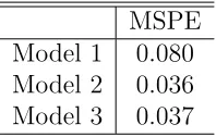
To compare models, we consider AIC , BIC and mean squared predicted error

based on Leave-one-out cross-validation method and we denote it by MSPE and is

defined as

MSPE = 1

n

n

i=1

(z_i −z_−i)2,

6 7 8 9 10 11 11 12 13 14 15 5 1 6 2 7 8 4 3 18 10 38 37 39 40 9 36 11 42 41 17 43 19 12 35 32 20

21 31 33 34

45 22 ₁₃

44 23

46 30 24

47 ₄₉ 29 25 16 14 28 48 15 27 26 [−1.72,2.95] (2.95,3.38] (3.38,3.66] (3.66,3.97] (3.97,4.23]

New Columbus OH: log transformation of crime rate per thousand households, 1980

6 7 8 9 10 11

11 12 13 14 15 [−1.72,2.95] (2.95,3.38] (3.38,3.66] (3.66,3.97] > 3.97

Predicted log transformed crime rate Model 2: ML method

6 7 8 9 10 11

11 12 13 14 15 [−1.72,2.95] (2.95,3.38] (3.38,3.66] (3.66,3.97] > 3.97

Predicted log transformed crime rate Model 3: ML method

Figure 3: Predicted Log transformed crime rate of Columbus OH (Model 2 and Model

Histogram of as.vector(res.new.c

residuals:log(crime rate)

Frequency

−6 −4 −2 0 1

0

5

15

25

−2 −1 0 1 2

−5

−3

−1

1

Normal Q−Q Plot

Theoretical Quantiles

Sample Quantiles

6 7 8 9 10 11

11 12 13 14 15 <=−0.236 (−0.236,−0.064] (−0.064,0.109] (0.109,0.443] (0.443,1.82]

Columbus OH: residual of log(crime rate) Model 2: ML method

Histogram of as.vector(res.new.d

residuals:log(crime rate)

Frequency

−6 −4 −2 0 1

0

5

10

20

−2 −1 0 1 2

−5

−3

−1

1

Normal Q−Q Plot

Theoretical Quantiles

Sample Quantiles

6 7 8 9 10 11

11 12 13 14 15 <=−0.236 (−0.236,−0.064] (−0.064,0.109] (0.109,0.443] (0.443,1.82]

Columbus OH: residual of log(crime rate) Model 3: ML method

Figure 4: Residual plots of log transformed crime rate of Columbus OH (Model 2 and

the predicted values, the best linear unbiased predictor (BLUP) (Schabenberger and

Gotaway, 2005) is considered and is given by

Model 1. X_iβ

Model 2. X_iβ+ρ

n

j=i

˜

w_ij(z_j −X_jβ)

Model 3. X_iβ+δ₁

n

j=1

˜

w(1)_ij z_j−X_jβ+δ₂

n

j=1

˜

w(2)_ij z_j −X_jβ.

First, from Table 5, we observe that AIC and BIC of CAR error model are smaller

than those of DCAR. Also, in Table 6, we observe that MSPE of Model 2 is the

smallest. However, AIC and BIC of DCAR error model are not quite nominally

different from those of CAR error. Also, MSPE of Model 3 (0.037) is very close to

that of Model 2 (0.036). From Figure 3 and 4, we observe that the predicted value

based on CAR error model appears to smooth out the log transformed crime rate

over Columbus, OH. Also, from residual plots of Model 2 (CAR error model), we

observe that residuals form blocks in the NW/SE direction. However, the predicted

value based on CAR error model appears to have higher rate in NW/SE direction

than NE/SW direction. From residual plots of Model 3 (DCAR error model), we

observe that residuals seem not to have any trend over study area. Therefore, we

conclude that the log-transformed crime rate of Columbus, OH has different spatial

dependence for neighbors in NW/SE direction and that of NE/SW direction. This

matches with the conclusion of Anselin who used two separate models to capture the

MSPE

Model 1 0.080

Model 2 0.036

Model 3 0.037

Table 6: Mean Squared Predicted Error of Leave-one-out method (MSPE_L)

5

Extensions and future work

DCAR model as an extension of CAR model, captures the directional spatial

depen-dence in addition to distance specific correlation. The DCAR model is also found

to be as efficient as the CAR model when data are generated from the CAR model.

However, CAR models usually fail to capture the directional effects when data is

generated from DCAR or other anisotropic model. Our model proposed in (6) can be

extended to more than two directions and one may similarly fit models of the type

Z ∼N_nXβ, σ2(I−

M

k=1

δ_kW˜ (k))−1D,

where ˜W(k) denote the matrices of weights specific to k-th directional effect. Our

current work involves the creation of even generated model that estimate the ˜W(k)’s

adaptively from the data and will be published else where.

Appendix A: Lemmas

Lemma 2 Let A =a_ij be a n×n matrix. If a_ii > _j=i|a_ij| for all i, then A is positive definite.

Lemma 3 Jacobi’s formula: Let B be n×n matrix. Then, d|B| = Tr(Adj(B)dB), in which Adj(B)is the adjugate of the matrixB_n×n anddB is its differentiable, where

| · | is determinant of matrix.

Proof: Given ann×n matrixB={b_ij}, its adjugate Adj(B) = A={a_ij}is defined as

a_ij = (−1)i+j|B without itsjth row and ith column|

so that AB = BA = |B|I. a_ij is the cofactor of b_ji in |B|, so a_ij is a polynomial

function of the elements of B but independent of b_jk and b_ki for all k. In |B| =

kbikaki, each elementbij is linearly multiplied by its cofactoraji, so∂|B|/∂bij =aji.

Thus,

d|B|=

j i

(∂|B|/∂b_ij)db_ij =

j i

a_jidb_ij = Tr(Adj(B)·dB).

Lemma 4 If Rank(B_n×n) =n (full rank), d log|B|= Tr(B−1dB).

Proof: See Section 10.8 of Graybill (1969).

Lemma 5 Let A be an n×n matrix with all real characteristic roots and let exactly

h (0< h≤n) of them be nonzero; then

[tr(A)]2 ≤h·tr(A2).

Proof of Lemma: See p.228-229 of Graybill (1969).

Appendix B: Proof of Theorem 2

To show that MLE of Gaussian DCAR model is asymptotically normal and weakly

hence Condition (iv) of Theorem 1 holds. We note that ˜W can be expressed asDW.

Similarly, ˜W(1) =DW₁ and ˜W(2) =DW₂. We now show that Conditions (i)-(iii) of

Theorem 1 are satisfied by the DCAR model.

Condition (i):For DCAR model, the variance covariance matrix Σis symmetric and positive definite if max(|δ₁|,|δ₂|)<1. Let 0< λ₁ < λ₂ <· · ·< λ_n be the eigenvalues

of A∗(δ)−1D. We can express the determinant of Σas |Σ|=σ2nn_i=1λ_i and that of

Σ−1 as |Σ−1| =σ−2nn_i=1λ1

i. As 1

λ1 is the largest eigenvalue ofD−1A∗(δ), we have

D−1 −δ₁W₁ −δ₂W₂x = _λ11 x, for some ||x|| = 1. Thus, xTD−1x−δ₁xTW₁x−

δ₂xTW₂x= _λ11. As xTD−1x=n_i=1m_ix2_i ≤m_(n), so it follows that lim supλ_n <∞.

|Σ₍₁₎| =|A∗(δ)−1D| =n_i=1λ_i. Thus as it is shown above, lim|λ1_n| = limλ_n =C =

C₁ <∞. For Σ₍₂₎, Σ₍₂₎ = σ2A∗(δ)−1W˜ (1)A∗(δ)−1D =σ2A∗(δ)−1DW(1)A∗(δ)−1D. Thus, the determinant of Σ₍₂₎ is |Σ₍₂₎|=σ2n|A∗(δ)−1D||W(1)||A∗(δ)−1D|

= σ2n n_i=1λ2_i|ξ_i(1)|, where ξ(1)_i ’s are eigenvalues of symmetric matrix W(1). Here,

based on Theorem 1 in Lancaster and Tismenetsky (1985) p.359 that is for any

matrix norm, if A ∈Rn×n and λ_A is the eigenvalue of A then ||A|| ≥ λ_A, it can be

shown that |ξ_n(1)| ≤ ||W₁|| = n_i,j=1w_1ij ≤ max(m_i), so |ξ_n(1)| ≤ M∗, where |ξ_n(1)| = max(|ξ_i(1)|). Thus, lim|λ2_n| = limσ2nλ_n2|ξ(1)_n | = C₂ < ∞. Similarly, for Σ₍₃₎, Σ₍₃₎ =

the eigenvalues of Σ_(ij), we derive that

Σ₍₁₁₎ = 0

Σ₍₁₂₎ = Σ₍₂₁₎=A∗(δ)−1DW(1)A∗(δ)−1D Σ₍₁₃₎ = Σ₍₃₁₎=A∗(δ)−1DW(2)A∗(δ)−1D

Σ₍₂₂₎ = 2σ2A∗(δ)−1DW(1)A∗(δ)−1DW(1)A∗(δ)−1D Σ₍₃₃₎ = 2σ2A∗(δ)−1DW(2)A∗(δ)−1DW(2)A∗(δ)−1D Σ₍₂₃₎ = 2σ2A∗(δ)−1DW(1)A∗(δ)−1DW(2)A∗(δ)−1D.

Thus, based on above results,

lim|λ11_n|= 0

|Σ₍₁₂₎| = |Σ₍₂₁₎|=

n

i=1

λ2_i|ξ(1)_i | ⇒lim|λ12_n|= lim|λ21_n|=C₁₂ =C₂₁=C₂ <∞

|Σ₍₁₃₎| = |Σ₍₃₁₎|=

n

i=1

λ2_i|ξ(2)_i | ⇒lim|λ13_n|= lim|λ31_n |=C₁₃ =C₃₁=C₃ <∞

|Σ₍₂₂₎| = (2σ2)n

n

i=1

λ3_i|ξ_i(1)|2 ⇒lim|λ22_n |= lim 2σ2λ3_n|ξ_n(1)|2 =C₂₂<∞

|Σ₍₃₃₎| = (2σ2)n

n

i=1

λ3_i|ξ_i(2)|2 ⇒lim|λ33_n |= lim 2σ2λ3_n|ξ_n(2)|2 =C₃₃<∞

|Σ₍₂₃₎| = |Σ₍₃₂₎|= (2σ2)n

n

i=1

λ3_i|ξ_i(1)||ξ_i(2)|

⇒ lim|λ22_n|= lim 2σ2λ3_n|ξ_n(1)||ξ(2)_n |=C₂₃=C₃₂ <∞.

Condition (ii):For the Euclidean norm of Σ_(i), ||Σ_(i)||2 ≤ _ln₌₁(λi_l)2 ≤ n(λi_n)2. Thus, ||Σ_(i)||−2 ≥ _n(λ1i

n)2. Here, λ

i

n converges to a finite constant as n → ∞ for all

i= 1, . . . , k forα = 1₂. Therefore, ||Σ_(i)||−2 =O(n−12−α) for all i= 1, . . . , k.

i, j = 1, . . . , k are

t₁₁ = nσ−4

t₁₂ = t₂₁=σ−2tr(W(1)A∗(δ)−1D) t₁₃ =t₃₁=σ−2tr(W(2)A∗(δ)−1D)

t₂₂ = tr(W(1)A∗(δ)−1DW(1)A∗(δ)−1D) t₃₃ =tr(W(2)A∗(δ)−1DW(2)A∗(δ)−1D)

t₂₃ = t₃₂=tr(W(1)A∗(δ)−1DW(2)A∗(δ)−1D).

For the ease of notation, let T_l=W_lA∗(δ)−1D for l= 1,2. Then,

a_ii = lim{t_ii/(t_iit_ii)1/2}= 1 for i= 1,2,3

a₁₂ =a₂₁= lim

tr(T1)2 ntr(T1T1)

_1/2

⇒a₁₂ =a₂₁= lim

1 ntr(T₁T₁₎

tr(T₁₎₂

_1/2

.

Here, by Lemma 5, tr(T1T1)

tr(T1)2 ≥

1

h (0< h≤n). Thus, a12=a21= 0.

a₁₃ =a₃₁= lim

1 ntr(T₂T₂₎

tr(T2)2

_1/2

.

Similarly, by Lemma 5, a₁₃=a₃₁ = 0.

a₂₃ =a₃₂ = lim

1 tr(T₁T₁₎tr(T₂T₂₎

tr(T1T2)2

_1/2

. For denominator, we consider eigenvalues

of A∗(δ)D and W_l for l= 1,2, then we express the denominator as

tr(T₁T₁)tr(T₂T₂)

tr(T₁T₂)2

_1/2

=

_n

i=1λ2i(ξi(1))2

_n

i=1λ2i(ξi(1))2

_n

i=1λ2i|ξi(1)||ξi(2)|

≤ nλ2n|ξn(1)| ·nλ2n|ξn(2)|

λ₁2n_i=1|ξ_i(1)||ξ_i(2)| =n

2λn

λ₁

2 ₁

i=1|ξ

(1)

i |

|ξn(1)|

|ξ(2)_i | |ξ(2)n |

,

where, |ξ_n(l)|= max(|ξ_i(l)|) for l = 1,2. As n → ∞, n2

λn λ1 ₂ 1 P

i=1|ξ (1)

i | |ξ(1)_n |

|ξ(2)_i | |ξ(2)_n |

→ ∞,

because |ξi(l)|

Therefore, A = [a_ij] = I_3×3 is an identity matrix, so it is nonsingular. Thus by Theorem 2, we note that MLE’s of Gaussian DCAR model are consistent and

asymptotically normal.

References

Akaike, H. (1974) “A new look at statistical model identification,”IEEE Transactions

on Automatic Control 19, 716-723.

Anselin, Luc. (1988) Spatial econometrics: methods and models, Kluwer Academic

Publishers.

Besag, J. (1974) “Spatial interaction and the statistical analysis of lattice systems”(with

discussion), Journal of the Royal Statistical Society, Series B 36, 192-236.

Breslow, N. E. and Clayton, D. G. (1993) “Approximate inference in generalized

lin-ear mixed models,” it Journal of the American Statistical Association 88, 9-25.

Brook, D. (1964) “On the distinction between the conditional probability and the joint

probability approaches in the specification of nearest-neighbour systems,”Biometrika

51, 481-483.

Byrd, R. H., Lu, P., Nocedal, J. and Zhu, C. (1995) “A limited memory algorithm

for bound constrained optimization,”SIAM Journal of Scientific Computing

16,1190-1208.

Cliff, A. D. and Ord, J. K. (1981) Spatial Processes: Models & Applications, Pion

Limited.

Cressie, N. (1993) Statistics for Spatial Data, John Wiley & Sons, Inc.

Efron, B. and Hinkley, D. V. (1978) “Assessing the accuracy of the maximum

457-482.

Graybill, F. A. (1969)Introduction to Matrices with Applications in Statistics, Wadsworth

Publishing Company.

Lancster, P. and Tismenetsky, M. (1985) The Theory of Matrices, Second Edition,

Academic Press.

Mardia, K. V. and Marshall, R. J. (1984) “Maximum likelihood estimation of models

for residual covariance in spatial regression,” Biometrika 71, 135-146.

Miller, H. J. (2004) “Tobler’s first law and spatial analysis,”Annals of the Association

of American Geographers 94, 284-295.

Ord, K. (1975) “Estimation methods for models of spatial interaction,” Journal of

the American Statistical Association 70, 120-126.

Ortega, J. M. (1987) Matrix Theory, New York:Plenum Press.

Schabenberger, O. and Gotaway, C. A. (2005) Statistical Methods for Spatial Data

Analysis, Chapman & Hall/CRC.

Schwartz, G. (1978) “Estimating the dimension of a model,” Annals of Statistics 6,

461-464.

Stone, M. (1977) “An asymptotic equivalence of choice of model by cross-validation

and Akaike’s criterion,” Journal of the Royal Statistical Society, Series B39, 44-47.

Sweeting, T., J. (1980) “Uniform asymptotic normality of the maximum likelihood

estimator,” Annals of Statistics 8, 1375-1381.

van der Linde, A., Witzko, K.-H. and Jockel, K.-H. (1995) “Spatio-temporal analysis

of mortality using splines” Biometrics 4, 1352-1360.

Wahba, G. (1977) “Practical approximate solutions to linear operator equations when