Impact of Sediment Processes on Water Quality in the Neuse River Estuary

Report No. 429

IMPACT OF SEDIMENT PROCESSES ON WATER QUALITY IN THE NEUSE RIVER ESTUARY

By

Yonghong Nie, Marc J. Alperin

Department of Marine Sciences

UNC-WRRI-429

The research on which this report is based was supported by funds provided by the North

Carolina General Assembly through the North Carolina Department of Environment and Natural Resources.

Contents of this publication do not necessarily reflect the views and policies of the WRRI, nor does mention of trade names or commercial products constitute their endorsement by the WRRI or the State of North Carolina.

This report fulfills the requirements for a project completion report of the Water Resources Research Institute of The University of North Carolina. The authors are solely responsible for the content and completeness of the report.

ACKNOWLEDGMENTS

iii ABSTRACT

A primary control on the estuarine nitrogen cycle involves interactions between the water

column and the sediments. These interactions are particularly important in shallow, slow-flowing estuaries like the Neuse where a large portion of the organic matter produced in the water

column reaches the sediment surface. Although time delays between deposition and

TABLE OF CONTENTS

ACKNOWLEDGEMENTS ………... ii

ABSTRACT ………. iii

TABLE OF CONTENTS ……….. iv

LIST OF FIGURES ………... v

LIST OF TABLES ……… vi

SUMMARY AND CONCLUSIONS ……….. vii

RECOMMENDATIONS ………... viii

INTRODUCTION ………. 1

SEDIMENT PROCESS MODEL ……….… 3

Diffusive Boundary Layer ………. 3

Sediment Processes …………...………. 3

Boundary Conditions ………. 9

Model Calibration ……….. 9

MODEL RESULTS AND DISCUSSION ………...…… 12

Impact of Reduced Nitrogen Loading on Benthic Fluxes ………... 12

Impact of Bottom Water Hypoxia on Benthic Fluxes ………. 14

Impact of Bottom Current on Benthic Fluxes ……….. 15

CONCLUSIONS ………. 19

REFERENCE LIST ………. 20

v

LIST OF FIGURES

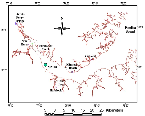
Figure 1. Map of the Neuse River estuary showing station MM70 ……….. 1

Figure 2. Model fit for sediment from station MM70 ……… 10

Figure 3. Modeling results for simulating POC flux reduction ……….. 13

Figure 4. Modeling results for simulating anoxic condition ………... 15

Figure 5. Current velocity variation case study I ……… 16

Figure 6. Current velocity variation case study II ………... 17

LIST OF TABLES

vii

SUMMARY AND CONCLUSIONS

Sediment-water column interactions in the Neuse River estuary are highly nonlinear and characterized by numerous positive and negative feedbacks between master variables (such as nitrogen loading and sediment organic matter deposition) and response variables (such as

internal cycling of nitrogen and total oxygen demand). The sediment diagenesis model presented here is a tool for making quantitative predictions of how the sediment system, and resulting benthic fluxes, respond to various scenarios involving changes in the master variables. The most important results from the sediment model are as follows:

1. Sediment oxygen demand responds slowly to a sudden reduction sedimentary organic matter deposition. This is because the sediments contain a large repository of reactive organic that serves as a time-release source of oxygen demand. Following a reduction of organic matter deposition, it will take 15 years for the sediment oxygen demand to decrease to 50% of its steady-state value.

2. The reduction in the steady-state benthic oxygen flux is not proportionate to the reduction in SOM deposition. For example, a 30% reduction in SOM flux translates to only a 20% reduction in benthic oxygen flux.

3. The reduction in the steady-state benthic ammonium flux is more than proportionate to the reduction in SOM deposition. For example, a 30% reduction in SOM flux

translates to a 73% reduction in benthic ammonium flux.

4. Reduced SOM deposition will shift the nitrogen species released from the sediments in favor of more nitrate and less ammonium.

5. Episodic hypoxia and anoxia in the bottom water result in elevated benthic fluxes of reactive nitrogen to the water column.

RECOMMENDATIONS

1. Exchange of carbon, nitrogen, and oxygen between the water column and the sediment must be an integral part of any estuarine water quality model.

2. The “lifetime” of sedimentary organic matter is the key variable for defining the rate at which the estuary will respond to changes in nitrogen loading. Hence, more work is needed to better constrain this variable in the Neuse River estuary.

INTRODUCTION

In this report, we discuss the development and application of a sediment process model that simulates and predicts the impact of sediment processes on water quality in the Neuse River estuary. Emphasis has been placed on capturing the details of the sediment-water interface—in particular, the diffusive boundary layer—in order to accurately simulate the impact of bottom water currents and concentrations on sediment processes and benthic fluxes.

This sediment model is applied in Neuse River estuary in North Carolina, USA (Figure 1). The Neuse River estuary shows many symptoms of an over-productive estuary: algal blooms, bottom water anoxia, and fish kills. Like most coastal ecosystems, primary production in the Neuse River estuary is generally limited by nitrogen (Paerl 1987; Paerl et al. 1990; Rudek et al. 1991). Anthropogenic nitrogen loading to the Neuse River basin has more than doubled since 1960 due to rapid growth in population and intensive agriculture (Stanley 1997). Although the link

between increased watershed nitrogen loading and phytoplankton biomass within the estuary is difficult to establish (e.g., Stanley et al. 2000; Stow et al. 2001), there is a widespread perception that impaired water quality within the Neuse River estuary is related to cultural eutrophication.

Figure 1. Map of the Neuse River estuary showing station MM70.

In an attempt to reduce primary production in Neuse River estuary, the North Carolina General Assembly has enacted legislation requiring a 30% reduction in nitrogen loading. While it is generally agreed that reduced nitrogen input will result in lower productivity, the long-term impact and the estuarine response time to nitrogen reduction are difficult to predict. This is because nitrogen is recycled through numerous biogeochemical compartments within the estuary before ultimately being removed by export, denitrification, or burial.

# # # # # # # # # # # # # # # # × × × × r r ú MM30 WP OR NRC NR3 UNC NRE NR1 NR5 NRH MM70 MM100 NR7 90-2 NR4 Oriental Havelock New Bern Minnesott Beach Northwest Creek Cherry Point Streets Ferry Bridge Pamlico Sound 35°00' 35°00' 35°10' 35°10' 77°10' 77°10' 77°00' 77°00' 76°50' 76°50' 76°40' 76°40' 76°30' 76°30' N

5 0 5 10 15 20 25 Kilometers

One of the primary controls on the estuarine nitrogen cycle is interaction between the water column and the sediments. This interaction is particularly important in shallow, slow-flowing estuaries like the Neuse where a large portion of the organic matter produced in the water column reaches the sediment surface (Suess 1980; Nixon 1981). In these systems, the benthic ammonium flux is an important, time-release source of recycled nitrogen to the water column. On the other hand, sediment denitrification is an important process for removing excess nitrogen from the estuary. Sediment-water column interactions also provide important controls on bottom-water hypoxia. Sediments in the Neuse River estuary are rich in organic matter and play an important role in the estuarine oxygen budget.

3

SEDIMENT PROCESS MODEL

DIFFUSIVE BOUNDARY LAYER

Since the model focuses explicitly on sediment-water column interactions, we need to simulate the fluid dynamics in the vicinity of the sediment-water interface. DE is the eddy diffusivity

created by turbulence in the water column. The height dependence of DE is given as (Van Driest

equation, Boudreau 2001):

        −                    − − + = 1 26 exp 1 4 1 2 2 / 1 2 2 2 Z Z

D_E ν κ , (1)

where ν is kinematic viscosity of water, κ is Von Karman’s constant (0.4), and Z is

dimensionless height, (Z = (xU*)/ν). The shear velocity (U*) is calculated according to Sternberg (1968) and Hickey et al. (1986):

) 000365 . 0 0526 . 0 33 . 2 (

10 3 U₁₀₀ U₁₀₀2

Cd = − − + , (2)

100 2 / 1 * ) (Cd U

U = . (3)

where Cd is the drag coefficient (unitless), and U100 is current velocity 1-meter above the sediment surface. The thickness of diffusive sublayer (δD) is calculated as:

0

/D

Sc=ν , (4)

* 3 / 2 0 ) ( 078 .

0 Sc U

D

D = ₋

δ , (5)

where Sc is the Schmitt number (Opdyke et al. 1987; Santschi et al. 1991; Boudreau 1997), and

0

D is the molecular diffusion coefficient.

SEDIMENT PROCESSES

The sediment model is based on a set of coupled, nonlinear differential equations that describe physical transport within the benthic boundary layer and surficial sediments, and chemical and biological processes associated with sedimentary organic matter (SOM) degradation (Rabouille and Gaillard 1991; Soetaert et al. 1996a; Boudreau 1997). The primary reactions involve microbially-mediated organic matter remineralization, including aerobic respiration,

denitrification, sulfate reduction, and methanogenesis. The secondary reactions involve oxidation of the reduced end-products from the primary biogeochemical reactions and include nitrification, methane oxidation, and Fe2+/sulfide oxidation. The primary and secondary reactions included in the model are summarized in the Appendix.

1984; Soetaert et al. 1996a, 1996b). SOM is represented by two degradable fractions (SOM1 and SOM2) with different first-order rate constants, and one refractory fraction (SOM3). Depth distributions of SOM pools are described by the following diagenetic equations:

(

)

1 1

1 1

[ ]

{(1 ) }

(1 ) [ ] {(1 ) [ ]}

(1 ) [ ]

B

SOM D

SOM _x SOM

k SOM

t x x

φ ρ

φ ρ ∂ − ∂ φ ρω _{φ ρ}

∂ − _∂ ∂ −

= − − −

∂ ∂ ∂ (6)

(

)

2 2

2 2

[ ]

{(1 ) }

(1 ) [ ] {(1 ) [ ]}

(1 ) [ ]

B

SOM D

SOM _x SOM

k SOM

t x x

φ ρ

φ ρ ∂ − ∂ φ ρω _{φ ρ}

∂ − _∂ ∂ −

= − − −

∂ ∂ ∂ (7)

3 3

[ ] [ ]

0 and 0

SOM SOM

t x

∂ ∂

= =

∂ ∂ , (8)

where DB (cm

2

yr-1_{) is the bioturbation coefficient,} ω _{(cm yr}-1) is the sedimentation rate, x (cm) is sediment depth, t (yr) is time, φ is sediment porosity, ρ is density of the sediment solid phase (2.5 g cm-3), k1 and k2 are the rate constants for degradation of SOM1 and SOM2,

respectively, and the brackets denote concentration.

Compaction is simulated by decreasing porosity exponentially with depth:

φ =(φ₀ −φ_∞)exp(−βx)+φ_∞ , (9) where φ₀ is the porosity at sediment-water interface, φ_∞ is porosity at infinite depth, and β is the scale-length coefficient. Values for porosity parameters (φ₀, φ_∞, β) are derived by fitting eq. (9) to measured porosity-depth distributions. Porosity in the water column is set to 1. An error function (erf) is used to maintain porosity continuity between the sediment and water column. The decrease in sedimentation rate with depth, due to compaction, is given by:

) 1 ( ) 1 ( φ φ ω ω − − ⋅ = ∞

∞ , (10)

where the subscript (∞) denotes values at infinite sediment depth.

Depth-dependence of the mixing coefficient (D_B) is described by the complementary error function (erfc) (Robbins 1986):

) ( 2 0 σ ML B B X x erfc D

D = − , (11)

where D_B0 is the bioturbation coefficient at sediment-water interface, X_ML is the depth where 5

. 0 / _B0 =

B D

D , and σ is a constant that controls dDB

5

bioturbation would not stop suddenly at a certain depth, but would decrease continuously with depth.

Equations (6), (7) and (8) assume that organic matter degradation rates are independent of the oxidant (oxygen, nitrate, sulfate, etc.). This assumption is widely used in diagenetic models (e.g., Dhakar and Burdige 1996; Soetaert et al. 1996a).

Our model assumes that aerobic respiration, nitrate reduction, sulfate reduction, and methane production are the dominant SOM decomposition pathways (organic matter oxidation via Fe and/or Mn oxides are assumed to be less important). Many studies have shown that the oxidant (electron acceptor) that provides the greatest free energy yield during organic matter

decomposition is used ahead of less energetic oxidants (Bender et al. 1977; Froelich et al. 1979; Emerson et al. 1980). Oxygen is the most favorable electron acceptor, followed by nitrate, and then sulfate. Fermentation, leading to methane production, generally occurs only after sulfate is depleted.

Error functions (and their complement) are used to simulate the sequential ordering of the organic matter decomposition reactions. Complementary error functions (f1 , f2 and f3) approach one when oxygen, nitrate and sulfate concentrations are less than limiting values for microbial uptake (O*, N*, and S*, respectively), and approach zero at higher values:

* * 2 2 1 * 2

1 if [ ] [ ]

0.5 erfc

0 if [ ]

O O O O O f O O σ  <  −   = ⋅ _{ ≈ }

  _ > , (12)

* * 3 3 2 * 3

1 if [ ]

[ ]

0.5 erfc ,

0 if [ ]

N NO N NO N f NO N σ − − −  <  −   = ⋅ _{ ≈ }

  _ > . (13)

2 * 2 * 4 4 3 2 * 4

1 if [ ]

[ ]

0.5 erfc .

0 if [ ]

S SO S SO S f SO S σ − − −  <  −   = ⋅ _{ ≈ }

  _ > (14)

Thus, f1 can be used to inhibit denitrification, sulfate reduction, and fermentation if oxygen concentrations are not limiting to aerobic bacteria. Likewise, the functions (1- f1), (1- f2) and (1- f3) serve to simulate the first-order dependence of respiration rates on oxidant concentrations as electron acceptors approach threshold levels.

These inhibition functions offer several advantageous over the more commonly used Michaelis-Menten equation (e.g., Devol 1978; Rabouille and Gaillard 1991; Boudreau 1996; Dhakar and Burdige 1996): (1) they provide a better fit to published oxygen uptake rate versus oxygen concentration data (Devol 1978); (2) they provide mathematical simplicity and computational efficiency; and (3) they assure electron balance by quantitatively linking organic matter decomposition and oxidant consumption.

1995; Soetaert et al. 1996a). The gradient parameters (σO , σN , and σS ) are set at 0.5 times the

limiting concentration.

The general diagenetic equation for oxygen includes terms for molecular diffusion, bioturbation, eddy diffusion, advection, and oxygen consumption:

2 2

2 2

1 1 1 1 1 2 2 4 4

1 1 2 2 2 2

[ ]

{ ( ) }

( [ ]) ( [ ])

(1 ){ [ ] [ ] 2 [ ] 2 [ ]}

[ ][ ] [ ][ ]

O

B S E

N Mo

ODU ODU

O

D D D

O _x O

t x x

f R k SOM R k SOM k NH k CH

k ODU O k ODU O

φ φ φυ φ φ φ + ∂ ∂ + + ∂ _∂ ∂ = − ∂ ∂ ∂ − − + + + − − (15)

where υ (cm yr-1) is pore water burial velocity. The relationship between ωand υ is:

x x ∂ − ∂ = ∂ ∂

− (φυ) [(1 φ)ω]. (16)

2

O S

D is the sediment diffusion coefficient for oxygen calculated from the molecular diffusion coefficient (D₀) and corrected for tortuosity (Ullman and Aller 1982):

0 2

D

DS =φ . (17)

R1 is a stoichiometric coefficient that relates organic matter oxidation and oxygen consumption. We assume that SOM has an oxidation state similar to carbohydrate so that one carbon is

degraded for each oxygen molecule (i.e., R1 equals 1). kN and kMo are rate constants for

nitrification and aerobic methane oxidation, respectively. As described above, the term (1 - f1) serves to simulate the cessation of aerobic processes when oxygen concentrations drop below the limiting value. ODU denotes oxygen-demanding units, which includes all the direct and indirect byproducts of sulfate reduction that could potentially consume oxygen (i.e., FeS, Fe2S, S2-, Fe2+). ODU1 represents soluble reduced compounds that are subject to molecular diffusion, while ODU2 represents compounds associated with the solid phase that are transported by

sedimentation and bioturbation. kODU1 and kODU2 are oxidation rate constants of ODU1 and

ODU2, respectively.

A similar diagenetic equation is used to describe nitrate concentration:

3 3

3 3

1 4 1 2 2 1 1 2 2 2

[ ]

{ ( ) }

( [ ]) ( [ ])

(1 )( [ ]) (1 ){ [ ] [ ]}

NO

B S E

N

NO

D D D

NO _x NO

t x x

f k NH f f R k SOM R k SOM

φ φ φυ φ φ − − − − + ∂ ∂ + + ∂ _∂ ∂ = − ∂ ∂ ∂ + − − − +

7

function that makes denitrification only occur in the presence of nitrate. Coupling f1 and f2 in eq. (18) assures that denitrification is limited by nitrate and is inhibited by oxygen.

The diagenetic equation for total ammonium is: 4

4 4

4

4 4

3 1 1 2 2 1 4

( ) ( [ ]) [ ] { } 1 1 ( [ ]) ( [ ]) ( [ ]) 1 1 1

{ [ ] [ ]} (1 )( [ ])

NH

ad B B S E

ad ad

ad

ad ad

N

K D NH D D D NH

K x K x

NH

t x

K

NH NH

K x K x

R k SOM k SOM f k NH

φ φ φ φυ φω φ φ + + + + + + + + + ∂ ∂ ∂ ⋅ + ⋅ + ∂ + ∂ ∂ = ∂ ∂ ∂ ∂ − − + ∂ + ∂ + + − − (19)

where NH4+

S

D is the diffusion coefficient for ammonium, R3 is a stoichiometric coefficient dependent on the C:N ratio of the degradable sedimentary organic matter (i.e., R3 equals N:C ratio), and Kad is the dimensionless adsorption coefficient for ammonium calculated from the

distribution coefficient of ammonium between solid matter and pore water (KD (mL g-1)):

∞ ∞ − = φ φ ρ1 D ad K

K . (20)

We assume that Kad is constant and independent of depth (Boudreau 1996, Van Cappellen and

Wang 1996). Total ammonium produced in bulk sediment must be corrected for adsorption in order to calculate the ammonium concentration in the pore water.

The diagenetic equation for sulfate is: 2 4 2 4 2 2 4 4

1 2 3 3 1 1 3 2 2 4

[ ]

{ ( ) }

( [ ]) ( [ ])

(1 ){ [ ] [ ] [ ]}

SO

B S E

Ma

SO

D D D

SO _x SO

t x x

f f f R k SOM R k SOM k CH

φ φ φυ φ − − − ∂ + + ∂ − ∂ _∂ ∂ = − ∂ ∂ ∂ − − + +

, (21)

where SO42−

S

D is the diffusion coefficient for sulfate, R3 is a stoichiometric coefficient that relates organic matter oxidation and sulfate consumption (i.e., R3 equals ½), the term f1f2(1- f3) assures that sulfate reduction occurs only occur when oxygen and nitrate are used up and sulfate is abundant, and

a

M

The diagenetic equation for methane is:

4 4

4 4

1 2 3 4 4 1 1 4 2 2

1 4 1 2 3 4

[ ]

{ ( ) }

( [ ]) ( [ ])

(1 ){ [ ] [ ]}

(1 ) [ ] (1 ) [ ]

CH

B S E

Mo Ma

CH

D D D

CH _x CH

t x x

f f f f R k SOM R k SOM

f k CH f f f k CH

φ φ φυ φ φ φ ∂ ∂ + + ∂ _∂ ∂ = − ∂ ∂ ∂ + − + − − − −

, (22)

where CH4

S

D is the diffusion coefficient for methane, R4 is a stoichiometric coefficient that relates organic matter oxidation and methane production (i.e., R3 equals ½). The term 1- f4 partitions methane into a gas phase when the porewater methane concentration exceeds in situ saturation.

The diagenetic equation for total dissolved CO2 (ΣCO2) is:

2 2

2 2

1 1 2 2

[ ]

{ ( ) }

( [ ]) ( [ ])

{ [ ] [ ]}

CO

B S E

CO

D D D

CO _x CO

t x x

k SOM k SOM

φ φ φυ φ ∂ Σ ∂ + + ∂ Σ _∂ ∂ Σ = − ∂ ∂ ∂ + +

. (23)

The diagenetic equation for ODU1 (dissolved oxygen demand) is:

1 1

1 1

1 1 2 3 3 1 1 3 2 2 1 1 2 1

[ ]

{ ( ) }

( [ ]) ( [ ])

(1 ){ [ ] [ ]} (1 ) [ ][ ]

ODU

B S E

ODU ODU

ODU

D D D

ODU _x ODU

t x x

f f f f R k SOM R k SOM f k O ODU

φ φ φυ φ ∂ ∂ + + ∂ _∂ ∂ = − ∂ ∂ ∂ + − + − − (24) The molecular diffusion coefficient of Fe2+ is used as DSODU1, kODU1 is the rate constant for

ODU1 oxidation (taken as the rate constant of Fe2+ oxidation; Fossing e al. 2004), fODU1 is the fraction of ODU1 among the total ODU produced through sulfate reduction.

The diagenetic equation for ODU2 (particulate oxygen demand) is:

1 1 2 3 3 1 1

3 2 2 1 2 2

[ 2]

{(1 ) }

((1 ) [ 2]) ((1 ) [ 2])

(1 ) (1 ) (1 ){ [ ]

[ ]} (1 ) (1 ) [ ][ 2]

B

ODU

ODU ODU

D

ODU _x ODU

t x x

f f f f R k SOM

R k SOM f k O ODU

φ ρ φ ρ φ ρω φ ρ φ ρ ∂ ∂ − ∂ − _{= ∂ −}∂ − ∂ ∂ ∂ + − − − + − − −

, (25)

9 BOUNDARY CONDITIONS

The upper boundary is set 1-cm above sediment surface and the lower boundary is at 100-cm depth in the sediment. The spatial resolution of the model is depth-dependent; highest from –1 to 1 cm to catch the detail of aerobic and denitrification zones. SOM pools have flux conditions at the upper boundary. Concentrations of oxygen, ammonium, and nitrate at the upper boundary are used as upper boundary conditions. Bottom water concentrations of sulfate and ΣCO2 are

calculated from salinity. Methane, ODU1, and ODU2 are set to zero concentration at the upper boundary. For all the species, the lower boundary conditions are set to zero concentration gradient.

MODEL CALIBRATION

Many parameters in the sediment model are directly or indirectly determined from data collected at ModMon station MM70 (Figure 1). MM70 is located in the middle of the Neuse Estuary and sediment at this site is more organic-rich relative to other areas in the estuary. We use this station as our test site because it is located in a region of the estuary that is most subject to hypoxia, algal blooms, and fish kills.

The measured parameters include: sedimentation rate, bioturbation coefficient, bioturbation depth, porosity, C:N ratio of SOM in the upper 3 cm of sediment, and ammonium adsorption coefficient. For example, sedimentation rate and bioturbation coefficient have been determined using geochronological tracers (210Pb and 137Cs), the C:N ratio of the degradable organic matter in the upper 3 cm of sediment has been estimated from ammonium and ΣCO2 production rate experiments, and ammonium adsorption coefficients have been determined by potassium

displacement studies. Model parameters that have not been measured are calibrated by fitting the model-generated concentration and reaction rate profiles with measured data in order to optimize the values of the parameters. Adjustable parameters include: (1) fluxes of SOM1 and SOM2 to the sediment; (2) degradation rate constants for SOM1 and SOM2 (k1 and k2, respectively); (3) nitrification rate constant (kN); (4) rate constants for aerobic and anaerobic methane oxidation

(k_Mo and a

M

k ); (5) C:N ratio of the SOM2; and (6) fraction of ODU1 among total ODU.

The sediment model is run to a quasi-steady state by allowing bottom water temperature, salinity, oxygen, nitrate, and ammonium to vary seasonally without inter-annual variability. At quasi-steady-state, model-generated concentration profiles for any species vary from month to month, but are consistent from year-to-year. Adjustable parameters in the sediment model are tuned as follows: the depositional flux and rate constant for SOM2 are constrained by measured ΣCO2, sulfate, and methane profiles and denitrification rate measurements; the depositional flux and rate constant for SOM1 is determined by oxygen concentration profile measured by

microelectrode; the rate constant for nitrification (kN) is constrained by the measured benthic

ammonium flux; rate constants for aerobic and anaerobic methane oxidation (k_Mo and a

Results of the calibrated model for sediment from MM70 are shown in Figure 2, and the calibrated model parameters are summarized in Table 1.

-0.1

0

0.1

0.2

0 5 10 15

POC (%) D ep th ( cm ) -0.1 0 0.1 0.2

0 150 300

O2 (uM)

-1

0

1

2

0 10 20

Nitrate (uM) 0 5 10 15 20

5 10 15

POC (%) D ep th ( cm ) 0 5 10 15 20

0 1 2 3

Am m onium (m M) 0 5 10 15 20

0 10 20 30

DIC (m M) 0 5 10 15 20

0 5 10 15

Sulfate (m M) 0 5 10 15 20

0 1 2 3

Methane (m M)

Reaction Rate (µM d-1)

0

5

10

15

20

0 1500 3000

GRR D ep th ( cm ) 0 5 10 15 20

0 125 250

APR 0 5 10 15 20

0 500 1000

DIC_PR 0 5 10 15 20

0 300 600

SRR 0 5 10 15 20

0 20 40

MPR

11

Table 1. Calibrated model parameters and parameters used in the simulations.

Model parameters Calibrated parameters

POC reduction Anoxia Current velocity test

0

φ 0.96783 0.96783 0.96783 0.96783

∞

φ 0.89735 0.89735 0.89735 0.89735

β (cm-1) 0.75696 0.75696 0.75696 0.75696

0 B

D (cm2 yr-1) 60 60 60 60

ML

X (cm) 28 28 28 28

∞

ω (g cm-2 yr-1) 0.2 0.2 0.2 0.2

SOM1 flux (mmol m-2 d-1) 24.8 Variable 24.8 24.8 SOM2 flux (mmol m-2 d-1) 13.3 Variable 13.3 13.3

SOM3 flux (mmol m-2 d-1) 36.5 36.5 36.5 36.5

1

k (yr-1) 100 100 100 100

2

k (yr-1) 0.6 0.6 0.6 0.6

C/N above 3 cm 4.5 4.5 4.5 4.5

C/N below 3 cm 6 6 6 6

ad

K (mL g-1) 8 8 8 8

N

K (yr-1) 80000 80000 80000 80000

o

M

K (yr-1) 106 106 106 106

a

M

K (yr-1) 0 0 0 0

T (ºC) Varies monthly 18 27.6 25.6

U100 (cm s-1) 5 5 5 Variable

Salinity (psu) 10 10 10 10

Water depth (m) 3.5 3.5 3.5 3.5

Benthic oxygen (µM) Varies monthly 284 Variable 192.8; 62.5; 0

Benthic nitrate (µM) Varies monthly 2.7 0.1 0.56

MODEL RESULTS AND DISCUSSION

Output from the sediment model includes: benthic fluxes of oxygen, nitrate, and ammonium, concentration profiles of all chemical species, and depth distributions of oxygen consumption rate, nitrification rate, denitrification rate, and organic matter degradation rates. Here, we use the sediment model to evaluate how sediment pools and processes respond to (1) reduced nitrogen loading, (2) sudden changes in bottom water oxygen concentration, and (3) variable bottom currents. For all applications, the quasi-steady state provides the initial conditions, and the model parameters used in each simulation are summarized in Table 1.

IMPACT OF REDUCED NITROGEN LOADING ON BENTHIC FLUXES

We assume that reduced nitrogen loading will translate into lower productivity in the estuary and less reactive SOM deposition to the sediment. Here, we conduct a sensitivity analysis to see how sediments respond to four SOM-flux reduction scenarios: 10%, 20%, 30% and 40% reduction of reactive SOM (i.e., SOM1 + SOM2). For each scenario, we consider two flux reduction patterns: instantaneous SOM flux reduction and gradual SOM flux reduction during a ten-year period. The year-round average bottom water temperature, benthic oxygen, nitrate, and ammonium

concentrations are used in the simulation.

Results of the simulation are shown in Figure 3. Instantaneous reduction of SOM deposition results in a relatively gradual reduction in the benthic oxygen flux. The relatively slow response time of the sediment oxygen demand to reduced SOM deposition (ca. 10 years) is due to the large repository of organic matter contained in the sediment. In contrast, denitrification and benthic ammonium flux both decrease rapidly in response to a sudden reduction in SOM deposition. Within 10-15 years after the start of the SOM flux reduction, benthic fluxes and denitrification rates are similar for instantaneous and gradual reduction scenarios. It takes the sediment column approximately 45 years to reach a new steady-state following a sudden or gradual reduction in SOM deposition.

Sediment oxygen demand decreases 5%, 11%, 20%, and 30% in response to SOM flux reductions of 10%, 20%, 30% and 40%, respectively. Though SOM deposition is the ultimate source of sediment oxygen demand, the benthic oxygen flux does not decrease linearly with SOM deposition. This is because reduced SOM flux results in deeper oxygen penetration allowing a more efficient oxidation of the upward diffusive flux of reduced solutes such as ammonium, sulfide, and ferrous iron.

Denitrification decreases 3%, 6%, 10%, and 15% for the four SOM reduction scenarios,

13 0 20 40 60 80

0 20 40 60

S O M D e p o s it io n ( mmo l C m

-2 d -1) 10% reduction 20% reduction 30% reduction 40% reduction Refractory SOM 0 20 40 60 80

0 20 40 60

Refractory SOM

0 0.5 1 1.5

0 20 40 60

B en th ic O 2 F lu x (g m

-2 d -1)

0 0.5 1 1.5

0 20 40 60

0 1 2 3

0 20 40 60

D e n it rif ic a tio n (mmo l N m

-2 d -1)

0 1 2 3

0 20 40 60

-3

-2

-1

0

0 20 40 60

B e n th ic A m m o n iu m (mmo l N m

-2 d -1)

-3

-2

-1

0

0 20 40 60

-6

-4

-2

0

0 20 40 60

Tim e (year)

The benthic ammonium flux also shows a nonlinear response to decreased SOM input. However, in this case the feedback in positive. The flux of ammonium from the sediments decreases by 27%, 52%, 73% and 88% in response to 10%, 20%, 30% and 40% reductions in SOM deposition, respectively. As discussed above, reduced SOM translates to deeper oxygen penetration and more effective nitrification.

The net result of 10%, 20%, 30%, and 40% reductions in SOM influx is to reduce the total benthic flux of reactive nitrogen by 13%, 26%, 39%, and 52%, respectively. The excess nitrogen removal is due to enhanced denitrification associated with stimulated nitrification resulting from deeper oxygen penetration.

In addition, there may be positive feedbacks resulting from sediment-water column coupling. Given that the benthic ammonium flux is equivalent to about 25% of the annually averaged nitrogen demand of primary producers (Alperin et al. 2000), we expect reduced primary

production and hence SOM deposition due to decreases in the benthic flux of reactive nitrogen. Furthermore, the ratio of ammonium:nitrate in the benthic flux decreases dramatically as a result of reduced SOM deposition. This shift will result in lower rates of water column nitrification, and possibly reduced oxygen demand in the bottom water.

IMPACT OF BOTTOM WATER HYPOXIA ON BENTHIC FLUXES

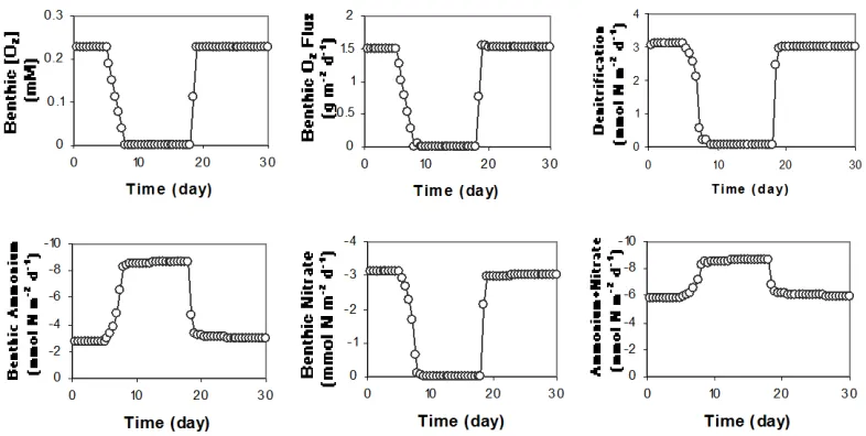
During the summer months, bottom water oxygen concentrations in the Neuse River estuary are highly variable in time, shifting from oxic to hypoxic or anoxic over periods of hours. In this experiment, we simulate the sediment response to a sudden period of bottom water anoxia that persists for two weeks. Bottom water temperature, benthic oxygen, nitrate and ammonium concentrations for month of July are used in this simulation.

Model results are summarized in Figure 4. Aerobic respiration, nitrification, and denitrification are restricted to the upper ~1 mm of the sediment column during the summer months. Molecular diffusion is quite fast over these space scales (ca. 10 min), so that benthic fluxes of oxygen, ammonium, and nitrate respond quickly to changes in bottom water oxygen. The benthic oxygen flux decreases in proportion to the oxygen concentration above the sediment-water interface. Oxygen depletion in the bottom water inhibits nitrification causing denitrification to nearly shut down (very little denitrification is supported by nitrate in the overlying water).

15

Figure 4. Modeling results for simulating anoxic condition.

IMPACT OF BOTTOM CURRENT ON BENTHIC FLUXES

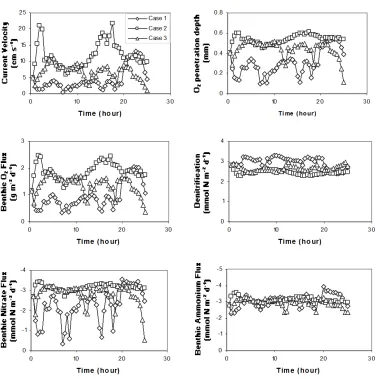
Current velocity in the bottom water (1-meter above bottom) is highly variable throughout the estuary (e.g., Figure 5, Luettich et al. unpublished data). Bottom current controls the thickness of the diffusive boundary layer and hence has an impact on sediment-water exchange and benthic processes. The sensitivity of the sediment system to bottom current introduces internal variability that must be resolved in order to discern trends associated with reductions in nitrogen loading and SOM deposition. Here, we test the sensitivity of the sediment system to bottom current for three periods, each lasting 25 hours:

Case 1: a period of relatively low velocity and low variability; Case 2: a period of high average velocity and high variability; Case 3: a period of moderate velocity and variability.

Since the currently velocity data are measured in June, bottom water temperature, benthic oxygen, nitrate and ammonium concentrations in the month of June are used in this simulation. Average oxygen penetration depth and benthic oxygen flux change dramatically in response to changes in bottom water velocity. However, the sediment response to bottom current is not linear. The average current velocity in Case 2 is almost three times that in Case 1, while oxygen penetration depth and oxygen consumption rate in Case 2 are only about two times that in Case 1. This is because oxygen penetration depth is controlled by the thickness of the diffusive boundary layer, and the thickness of the diffusive boundary layer is most sensitive to current velocity when the velocity is low. Case 2 has the highest average current velocity, highest

higher current velocity, oxygen penetrates deeper, forcing denitrification to greater depth. The benthic ammonium flux is nearly unchanged with current velocity.

Figure 6 shows how benthic fluxes and sediment processes respond to changes in current velocity. In general, oxygen penetration depth and benthic fluxes of oxygen and nitrate track bottom current velocity, while the denitrification rate and ammonium flux are relatively insensitive to bottom current velocity.

The combined effects of bottom water oxygen concentrations and changing bottom currents are simulated for Case 1. Three bottom water oxygen scenarios are tested: 80% oxygen saturation (192.8 µM), threshold of hypoxia (62.5 µM), and anoxia. The modeling results are shown in Figure 7. The sensitivity of the sediments decreases at lower bottom water oxygen

concentrations.

0 5 10 15 20 25

0 50 100 150 200 250 300 350 400

Time (hour)

C

u

rr

en

t vel

o

ci

ty (

cm

s

-1 ) Case

1

Case 2

17

19

CONCLUSIONS

Sediment-water column interactions in the Neuse River estuary are highly nonlinear and characterized by numerous positive and negative feedbacks between master variables (such as nitrogen loading and sediment organic matter deposition) and response variables (such as

internal cycling of nitrogen and total oxygen demand). The sediment diagenesis model presented here is a tool for making quantitative predictions of how the sediment system, and resulting benthic fluxes, respond to various scenarios involving changes in the master variables. The most important results from the sediment model are as follows:

4. Sediment oxygen demand responds slowly to a sudden reduction sedimentary organic matter deposition. This is because the sediments contain a large repository of reactive organic that serves as a time-release source of oxygen demand. Following a reduction of organic matter deposition, it will take 15 years for the sediment oxygen demand to decrease to 50% of its steady-state value.

5. The reduction in the steady-state benthic oxygen flux is not proportionate to the reduction in SOM deposition. For example, a 30% reduction in SOM flux translates to only a 20% reduction in benthic oxygen flux.

6. The reduction in the steady-state benthic ammonium flux is more than proportionate to the reduction in SOM deposition. For example, a 30% reduction in SOM flux

translates to a 73% reduction in benthic ammonium flux.

7. Reduced SOM deposition will shift the nitrogen species released from the sediments in favor of more nitrate and less ammonium.

8. Episodic hypoxia and anoxia in the bottom water result in elevated benthic fluxes of reactive nitrogen to the water column.

9. Variations in bottom current introduce internal variability in sediment-water column exchange processes. The benthic oxygen flux increases markedly with bottom current while denitrification slightly reduced at higher bottom water velocities. The benthic ammonium flux is controlled by processes well below the diffusive boundary layer and is little affected by bottom current.

REFERENCE LIST

Alperin, M. J., E. J. Clesceri, J. T. Wells, D. B. Albert, J. E. McNinch, and C. S. Martens. 2000. Sedimentary processes and benthic-pelagic coupling. In: Neuse River Estuary Modeling and Monitoring Project: Final Report—Monitoring Phase, R. A. Luettich, Jr. (Editor), Water Resources Research Institute Report, 63-105.

Bender, M. L., K. A. Fanning, P. N. Froelich, F. R. Heath, and V. Maynard. 1977. Interstitial nitrate profiles and oxidation of sedimentary organic matter in the eastern equatorial pacific. Science 198:605-609.

Billen, G. 1978. A budget of nitrogen recycling in North Sea sediments off the Belgian coast. Estuarine Coastal Mar. Sci. 7: 127-146.

Boudreau, B. P. 1996. A method-of-lines code for carbon and nutrient diagenesis in aquatic sediments. Computers & Geosciences. 22:479-496.

Boudreau, B. P. 1997. Diagenetic Models and Their Inplementation. Springer-Verlag, N. Y. Christian, R. R., J. N. Boyer, D. W. Stanley, and W. M. Rizzo. 1992. Network analysis of

nitrogen cycling in and estuary, p. 217-247. In C.J. Hurst(ed). Modeling the Metabolic and Physiologic Activities of Microorganisms, John Wiley and Sons, New York.

Devol, A. H. 1978. Bacterial oxygen uptake kinetics as related to biological processes in oxygen deficient zones of the oceans. Deep-Sea Res. 25: 137-146.

Dhakar, S. P. and D. J. Burdige. 1996. A coupled, non-linear, steady state model for early diagenetic processes in pelagic sediment. Am. J. Sci. 296: 296-330.

Dodd, R. C., P A. Cunningham, R. J. Curry, and S. J. Syichter. 1993. Watershed planning in the Albemarle-Pamlico Estuarine System, Report No. 93-01, Research Triangle Institute, Research Triangle Park, NC Department of Environment, Health, and Natural Resources. Emerson, S., R. Jahnke, M. Bender, P. Froelich, P. Klinkhammer, C. Bowser, and G. Setlock.

1980. Early diagenesis in sediments from the eastern equatorial Pacific. I. Pore water nutrient and carbonate results. Earth Planet. Sci. Lett. 49: 57-80.

Esteves, J. L., G. Mille, F. Blanc, and J. C. Bertrand. 1986. Nitrate reduction activity in a continuous flow-through system in marine sediments. Microb. Ecol. 12: 283-290. Fossing, H, Berg, P, Thamdrup, B, Rysgaard, S, Sørensen, H. M., and Nielsen, K. 2004. A

21

matter in pelagic sediments of the eastern equatorial Atlantic: suboxic diagenesis. Geochim. Cosmochim. Acta. 43:1075-1090.

Harned, D. A. and M. S. Davenport. 1990. Water-quality trends and basin activities and

characteristics for the Albemarle-Pamlico Estuarine System, NC and VA. Report 90-398, U.S. Geologic Survey, Raleigh, NC.

Harington, D. and D. Stotts. 2003. DeCo: A declarative coordination framework for scientific model federations. Technical Report TR03-017, Department of Computer Science, Univ. of North Carolina at Chapel Hill.

Hickey, B., E. Baker, and N. Kachel. 1986. Suspended particle movement in and around Quinault Submarine Canyon. Mar. Geol. 71:35-83.

Jørgensen, B. B., M. Bang, and T. H. Blachburn. 1990. Anaerobic mineralization in marine sediments from the Baltic Sea-North Sea transition. Mar. Ecol. Progr. Ser. 59: 39-54. Kemp, W. M., P. Sampie, J. Caffrey, M. Mayer, K. Henriksen, and W. R. Boynton. 1990.

Ammonium recycling versus denitrification in Chesapeake Bay sediments. Limnol. Oceanogr. 35:1545-1563.

Metcalf and Eddy Inc. 1979. Theoretical model for manganese distribution in calcareous sediment cores. J. Geophys. Res. 76: 2179-2186.

Murry, R. E., L. L. Parson, and M. S. Smith. 1989. Kinetics of nitrate utilization by mixed populations of denitrifying bacteria. Appl. Environ. Microbiol. 55: 717-721.

Nielsen, L. P., P. B. Christensen, N. P. Revsbech, and J. Sørensen. 1990. Denitrification and oxygen respiration in biofilms studied with a microsensor for nitrous oxide and oxygen. Microb. Ecol. 19: 63-72.

Nixon, S. W. 1981. Remineralization and nutrient cycling in coastal marine ecosystems. In: Nutrients and Estuaries, B.J. Nielson and L.E. Cronin (eds.), pp.111-138, Humana Press. Opdyke, B. N., G. Gust, and J. R. Ledwell. 1987. Mass transfer from smooth alabaster surfaces

in turbulent flows. Geophys. Res. Lett. 14:1131-1134.

Paerl, H. W. 1987. Dynamics of blue-green algal blooms in the lower Neuse River, North Carolina: Causative factors and potential controls. Report No. 229. Water Resources Research Institute. University of North Carolina, Raleigh.

Rabouille, C. and J. –F. Gaillard. 1991. Towards the EDGE: Early diagenetic global explanation. A model depicting the early diagenesis of organic matter, O2, NO3, Mn, and PO4.

Geochim. Cosmochim. Acta 55:2511-2525.

Robbins, J. A. 1986. A model for particle-selective transport of tracers in sediments with conveyor belt deposit feeders. J. Geophys. Res. 91: 8542-8558.

Rudek, J., H. W. Paeral, M. A. Mallin, and P. W. Bates. 1991. Seasonal and hydrologic control of phytoplankton nutrient limitation in the lower Neuse River Estuary, North Carolina. Mar. Ecol. Progr. Ser. 75:133-142.

Santschi, P. H., R. F. Anderson, M. Q. Fleisher, and W. Bowles. 1991. Measurements of diffusive sublayer thickness in the ocean by alabaster dissolution, and their implications for the measurements of benthic fluxes. J. Geophys. Res. 96:10641-10657.

Soetaert, K., P. M. J. Herman, and J. J. Middelburg. 1996a. A model of early diagenetic processes from the shelf to abyssal depths. Geochim. Cosmochim. Acta 60:1019-1040. Soetaert, K., P. M. J. Herman, and J. J. Middelburg. 1996b. Dynamic response of deep-sea

sediments to seasonal variations: a model. Limnol. Oceanogr. 41: 1651-1668. Sternberg, R. W. 1968. Friction factors in tidal channels with differing bed roughness. Mar.

Geol. 6:243-260.

Stow, C. A., M. E. Borsuk, and D. W. Stanley. 2001. Long-term changes in watershed nutrient inputs and riverine exports in the Neuse River, North Carolina. Wat. Res. 35: 1489-1499. Suess, R. 1980. Particulate organic carbon flux in the oceans: Surface productivity and oxygen

utilization. Nature, 288:260-263.

Ullman, W. J. and R. C. Aller. 1982. Diffusion coefficients in near-shore marine sediments. Limnol. Oceanogr. 27: 552-556.

Van Capppellen, P., J.-F. Gaillard, and C. Rabouille. 1993. Biogeochemical transformations in sediments: kinetic models of early diagenesis. In R. Wollast, F. T. Mackenzie and L. Chou [eds.], Interactions of C, N, P and S Biogeochemical Cycles and Global Change. Springer-Verlag. 401-445.

23

APPENDIX

1. CH₂O+O₂ →CO₂ +H₂O

2. 5CH₂O+4NO₃ +4H+ →2N₂ +5CO₂ +7H₂O

3. CH O SO H H2S CO2 H2O

2 4

2 2 2 2

2 + − + + → + +

H₂S > 2H+ +ODU 4. 2CH₂O→CH₄ +CO₂

5. NH₄+ +2O₂ →NO₃− +H₂O+2H+

6. CH4 +2O2 →CO2 +2H2O

7. CH₄ +SO₄2− →CO₂ +H₂S+2OH− 8. ODU +2O2 →ODU •O4