An Immersed Boundary Method for Simulating the Effects of Control Devices used in Mitigating Shock / Boundary-Layer Interactions

ABSTRACT

GHOSH, SANTANU. An Immersed Boundary Method for Simulating the Effects of Control Devices used in Mitigating Shock / Boundary-Layer Interactions. (Under the direction of Dr. Jack R. Edwards).

This work presents an immersed boundary (IB) technique for compressible, turbulent flows and applies the technique to simulate the effects of three different devices used in controlling oblique-shock / turbulent boundary-layer interactions – wedge shaped micro vortex generators (VG), an array of bleed holes, and aeroelastically deflecting mesoflaps. Both Reynolds averaged Navier-Stokes (RANS) and hybrid large-eddy / Reynolds-averaged Navier-Stokes (LES/RANS) turbulence closures are used with the IB technique.

Simulations of an impinging oblique-shock / boundary-layer interaction at Mach 2.45 with and without bleed flow control predict Pitot-pressure distributions which are in good agreement with experimental data. Flow control at two different bleed rates is considered, with the maximum bleed rate completely removing the separation region. Swirl strength probability density distributions, and Reynolds-stress predictions indicate that an effect of strong bleed rates is to accelerate the recovery of the boundary layer toward a new equilibrium state downstream of the interaction region.

An Immersed Boundary Method for Simulating the Effects of Control Devices used in Mitigating Shock / Boundary-Layer Interactions

by Santanu Ghosh

A dissertation submitted to the Graduate Faculty of North Carolina State University

in partial fulfillment of the requirements for the degree of

Doctor of Philosophy

Aerospace Engineering

Raleigh, North Carolina March, 2010

APPROVED BY:

_______________________________ ______________________________ Dr. J. R. Edwards Dr. H. A. Hassan

Committee Chair

DEDICATION

BIOGRAPHY

Santanu Ghosh was born on 5th August, 1978, to Asim Kumar Ghosh and Putul Ghosh in Kolkata, India. He did his initial schooling from Hartley’s High School in Kolkata, and then went to attend high school at St. Xavier’s College in the same city. After graduating from high school, Santanu joined Jadavpur University, Kolkata, to do his undergraduate studies in the area of Mechanical Engineering. It was at Jadavpur University, where he was first introduced to CFD by Dr. Achintya Mukhopadhyaya, whose approach towards teaching really impressed Santanu. After completing his graduation, Santanu joined Infosys, a leading software company in India in 2002. Here he worked for the next two years, and then went to University of Texas, Arlington, to pursue graduate education. He received his Masters degree in Mechanical Engineering from UTA where he did research in the area of stress analysis of electronic packages under the supervision of Dr. Brian H. Dennis. At this point, Santanu wanted to work in the area of CFD, in which he had an interest since his undergraduate days. He got an opportunity to work in this field at North Carolina State University, under the supervision of Dr Jack R. Edwards.

ACKNOWLEDGMENTS

Firstly I would like to express my gratitude and thankfulness to Dr. Jack R. Edwards for providing me with the opportunity to pursue graduate education at NC State, his patience with me, and the help and advice I have got from him in the past four years. His diligence, focus, and clarity of thinking are traits which I find to be admirable. I am also thankful to my committee members Dr. H. A. Hassan, Dr. M. A. Zikry, and Dr. T. Echekki for serving on my dissertation committee and providing help and inputs when I needed them. I also want to thank my ex-colleagues at NC State, Patrick, John, and specially Jung-IL, who were very helpful and co-operative.

I also must thank the NC State University High Performance Computing for providing computing resources and support. I would also like to thank the Air Force Office of Scientific Research for their funding support under grant FA9550-07-1-0191, monitored by Dr. John Schmisseur.

TABLE OF CONTENTS

LIST OF FIGURES ... ix

LIST OF TABLES ... xvi

NOMENCLATURE ... xvii

Chapter 1. Introduction ... 1

Chapter 2. Governing Equations ... 12

2.1 Time Averaging: Reynolds-Averaged Navier-Stokes (RANS) Equations ... 14

2.2 Menter k-ω / k-ε Model ... 19

2.3 Large Eddy Simulation... 20

2.5 Mixed Scale Model ... 23

2.6 Hybrid LES/RANS Methodology ... 23

Chapter 3. Numerical Methods ... 27

3.1 Discretization of Fluxes ... 27

3.2 LDFSS ... 29

3.3 Time Integration ... 33

3.4 LES/RANS: Initialization ... 34

3.5 LES/RANS Inflow Generation: Recycling/Rescaling ... 35

Chapter 4. Immersed Boundary Methodology ... 38

4.2 Interpolation Methods ... 43

4.2 Interpolation Point: Location and Data Construction ... 49

Chapter 5. Fluid-Structure Interaction ... 52

5.1 Structural Solver ... 53

5.2 Fluid-Structure Coupling... 57

Chapter 6. Flow Control: Vortex Generator ... 64

6.1 Case Studies ... 65

6.2 Problem Setup ... 66

6.3 Results ... 72

6.4 Conclusions ... 102

Chapter 7. Flow Control: Bleed Holes ... 104

7.1 Case Studies ... 105

7.2 Problem Setup ... 105

7.3 Results ... 112

7.4 Conclusions ... 132

Chapter 8. Flow Control: Aeroelastic Mesoflaps ... 134

8.1 Case Studies ... 135

8.2 Problem Setup ... 135

8.3 Results ... 140

8.4 Conclusions ... 164

LIST OF FIGURES

Fig. 1.1 Schematic of an oblique shock/boundary-layer interaction; Figure from Sandham et al. [2] ...2 Fig. 4.1 Cell classification scheme for immersed boundary method ...39 Fig. 4.2 Schematic showing the approximate nearest surface pointx_s for any band point

k

x and the signed distance function Fl

( )

closed circles : surface node points; Figure from Choi et al. [35] ...41 Fig. 4.3 Schematic of control volume used to define normal velocity component at band

cells ...46 Fig. 4.4 Schematic determination of the distance d_I between the interpolation point

I

x and surface node point for a given band point x_kusing the projected distance d_l

from neighbor points x_l to outward normal line based on surface normal vector n at the immersed surface node x_s; blue filled circle - band point to be interpolated with the information at neighboring points, hatched black and grey circle – field and band

points associated with the interpolation point data construction respectively. Figure from Choi et al. [35]...51 Fig. 5.1 Aeroelastic mesoflaps over a cavity for (a) subsonic flow and (b) supersonic flow

Fig. 5.2 a) 2-D view of a mesoflap rendered as an IB, b) structural model of a mesoflap as

a cantilevered beam ...54

Fig. 5.3 Schematic representation of interpolation scheme used in the reconstruction of surface loads on mesoflap upper and lower surfaces ...59

Fig. 6.1 A wedge shaped vortex generator ...64

Fig. 6.2 Schematic of Cambridge University wind tunnel showing the data stations, VG positions and shock generator (provided by H. Babinsky); inset shows IB rendition of a 3 mm VG ...67

Fig. 6.3 X-Y view of grid (near wall) used in Domain 1 ...70

Fig. 6.4 Plot of wind tunnel coordinates and spline fit ...70

Fig. 6.5 Inflow velocity profiles (X = 89 mm) ...73

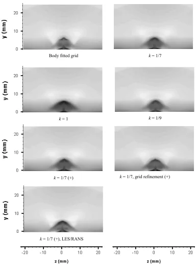
Fig. 6.6 Mach number contours at X = 111 mm for 6 mm VG placed in supersonic boundary layer; (+: continuity equation integrated in band cells) ...76

Fig. 6.7 Mach number contours at X = 199 mm for 6 mm VG placed in supersonic boundary layer; (+: continuity equation integrated in band cells) ...77

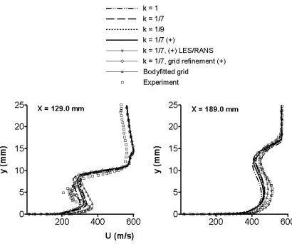
Fig. 6.8 Comparison of centerline axial velocity profiles for different formulations of the IB method, a body fitted grid and experimental data. (+: continuity equation integrated in band cells) ...78

Fig. 6.10 Comparison of axial velocity profiles for flow over 6 mm VG in idealized domain...80 Fig. 6.11 Comparison of axial velocity profiles for flow over 3 mm VG in idealized

domain (* = data averaged over a span wise filter of 2.5 mm, centered at the Z location) ...81 Fig. 6.12 Schlieren images of SBLI in wind tunnel using RANS model (left), and

experiment (right) ...84 Fig. 6.13 Near surface velocity contours at Y = 0.0025 mm (range: -5 m/s (dark) to 35

m/s) for SBLI in wind tunnel (contours reflected about centerline for clarity) ...84 Fig. 6.14 Near-surface streamtraces for SBLI in wind tunnel ...85 Fig. 6.15 Centerline surface pressure distributions for SBLI in wind tunnel (with/ without

micro VG array) ...87 Fig. 6.16 Centerline axial velocity profiles for SBLI in wind tunnel ...87 Fig. 6.17 Near-Surface velocity contours at Y = 0.0025 mm (range: -5 m/s (dark) to 35

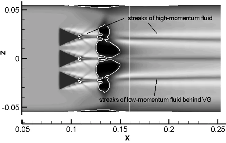
m/s) for SBLI with micro VG array in wind tunnel (contours reflected about the centerline for clarity)...89 Fig. 6.18 Near-surface streamtraces for SBLI with micro VG array in wind tunnel ...90 Fig. 6.19 Axial velocity profiles for SBLI with micro VG array in wind tunnel (* indicates

Fig. 6.21 Centerplane Mach number contours (idealized interaction without micro VG array) ...96 Fig. 6.22 Surface velocity contours (range: -5 m/s (dark) to 35 m/s) for idealized SBLI

(Menter SST RANS model) ...97 Fig. 6.23 Surface velocity contours (range: -5 m/s (dark) to 35 m/s) for idealized SBLI

(LES/RANS model) ...97 Fig. 6.24 Centerplane Mach number contours (idealized interaction with micro VG array) ...99 Fig. 6.25 Surface velocity contours (range: -5 m/s (dark) to 35 m/s) for idealized SBLI

with micro VG control (Menter SST RANS model) ...100 Fig. 6.26 Surface velocity contours (range: -5 m/s (dark) to 35 m/s) for idealized SBLI

with micro VG control (LES/RANS model) ...100 Fig. 6.27 Span-averaged axial velocity profiles for RANS and LES/RANS closures with

and without micro VG array (idealized interaction) ...101 Fig. 7.1 3-D view of bleed plate with an array of 90 degree through holes ...104 Fig. 7.2 Mesh around the IB rendition of a circular bleed hole ...109 Fig. 7.3 3-D view of flow over a perforated plate with active suction (Mach number

contours shown) ...113 Fig.7.4 X-Y view of flow over a perforated plate with active suction (Mach number

Fig. 7.6 Snapshot of centerplane temperature contours for oblique shock interaction

without bleed ...115

Fig. 7.7 Wall pressure distributions: shock / boundary-layer interaction without bleed ...116

Fig. 7.8 Pitot pressure distributions: shock / boundary-layer interaction without bleed ...117

Fig. 7.9 Snapshot of temperature contours with inset bleed plate: shock / boundary-layer interaction with bleed ...120

Fig. 7.10 Wall pressure distributions: shock / boundary-layer interaction with bleed; (*) - averaged at pressure tap locations ...121

Fig. 7.11 Pitot pressure distributions: shock / boundary-layer interaction with half-bleed ..123

Fig. 7.12 Pitot pressure distributions: shock / boundary-layer interaction with full-bleed...124

Fig. 7.13 Pitot pressure profiles at exit of bleed holes with full bleed ...125

Fig. 7.14 Bleed mass flux distribution ...126

Fig. 7.15 Mach number contours in bleed hole ...127

Fig. 7.16 Evolution of resolved turbulent kinetic energy through the interaction region ...129

Fig. 7.17 Evolution of Reynolds shear stress ru v¢ ¢ through the interaction region ...129

Fig. 7.18 Iso-surfaces of swirl strength (10000 s-1) for interactions with full bleed and no bleed ...130

Fig. 7.19 Evolution of swirl-strength probability density distributions ...131

Fig. 8.2 Snapshot of contour plots of axial velocity on an X-Z plane (close to surface) and pressure on an X-Y plane; iso-surface of zero axial velocity shown in blue on the near surface plane...141 Fig. 8.3 Snapshot of Mach number contours showing in white the zero axial velocity

boundary ...141 Fig. 8.4 Centerline wall pressure for SBLI without control ...143 Fig. 8.5 Centerline axial velocities for shock/boundary layer interaction without control ...143 Fig. 8.6 Streamwise turbulence intensity profiles at various streamwise locations; a)

inflow, b) interaction region, and c) downstream ...144 Fig. 8.7 Mach number contours for the converged configuration of the mesoflap array;

flaps are numbered from left (upstream) to right (downstream) ...148 Fig. 8.8 History of maximum deflection of each mesoflap ...148 Fig. 8.9 Mach number contours for shock/boundary layer interaction with control by

mesoflap array ...149 Fig. 8.10 Snapshots of Mach numbers contours; frames are spaced at intervals of 600

iterations ~ 0.09 ms ...151 Fig. 8.11 Snapshots of pressure contours; frames are spaced at intervals of 600 iterations ~

0.09 ms ...152 Fig. 8.12 Near surface (~ 1mm from wall) static pressure history with the time averaged

Fig. 8.13 Deflection history of the mesoflaps (represented by black lines) with the time-averaged positions shown in red ...155 Fig. 8.14 Deflection and interpolated net pressure load (on flap surfaces) comparisons for

the quasi-steady and dynamic modeling of the mesoflaps; loads - symbol, displacement - solid lines. ...155 Fig. 8.15 Frequency analysis of flap–response (blue) based on the displacement of the

edge of the flap; red lines: natural frequencies (four shown), black line: low frequency shock motion, green line: boundary layer turbulence frequency, pink line: frequency based on recirculation time in cavity ...157 Fig. 8.16 Centerline wall pressure for SBLI with control; pressure at the lower wall of

cavity is shown for the region of the mesoflap array (-5.6 to 5.6 on the X axis) ...159 Fig. 8.17 Centerline axial velocities for SBLI with control ...160 Fig. 8.18 Streamwise turbulence intensity profiles for SBLI with control at two

streamwise locations downstream of interaction ...160 Fig. 8.19 Time and span-averaged near surface (~ 1mm from wall) static pressure for the

LIST OF TABLES

Table 2.1 Model constant a

( )

shock interaction ...68 Table 6.2 Summary of cases ...72 Table 7.1 Free-stream and boundary-layer conditions for Willis, et al. [63] shock /

boundary-layer experiments ...107 Table 7.2 Free-stream and boundary-layer conditions for Willis, et al. [62] flat-plate

NOMENCLATURE

a1 = Menter BSL model constant

b = width of mesoflap

Cf = skin friction coefficient

CM = model constant for mixed scale model

Cp = specific heat at constant pressure

Cp = specific heat at constant volume

Cμ = Menter BSL model constant D = diameter of bleed hole

d = distance from nearest wall, or, distance from immersed surface

d- _{= normalized distance}

d + = normalized distance, or, wall coordinate

E = total energy per unit mass, or, modulus of elasticity of mesoflap material E, F, G = flux vectors in i, j, and k directions

F1, F2 = blending functions used in Menter BSL model

f = scaling function used in immersed-boundary formulation, or, load per unit area on mesoflap

g = scaling function used in immersed-boundary formulation

H = total enthalpy per unit mass

h = height of vortex generator

I = area-moment of inertia about neutral axis of mesoflap cross-section

K = coefficient or stiffness matrix used in structural solver

k = turbulent kinetic energy per unit mass, or, subgrid scale kinetic energy per unit mass, or, power law

L = depth of bleed hole, or, length of mesoflap

M = Mach number

n, ni = outward normal vector to immersed surface or cell face

n = coordinate normal to immersed surface

P = time averaged static pressure

Pt = Pitot pressure

Pr = Prandtl number

PrT = turbulent Prandtl number

p = static pressure

qi = heat flux vector

qTi = turbulent heat flux vector

SGS j

q = subgrid scale heat flux vector

q2 = estimate of subgrid kinetic energy Q = sonic flow coefficient

R = gas constant

Re = Reynolds number

r = recovery factor S = source vector

Sij = strain-rate tensor

T = temperature

t = time, or, thickness of mesoflap U = conservative variable vector u, ui = velocity vector

u, v, w = components of velocity in x, y, and z direction

un = velocity normal to cell face

uτ = friction velocity

V = primitive variable vector

W = blending function used in boundary layer scaling X, Y, Z = coordinates in computational domain

x = distance from leading edge of computational domain along X Symbols

α = model parameter for hybrid LES/RANS

β = model constant in Menter BSL model, or, Newmark parameter β* = model constant in Menter BSL model

Kleb

G = Klebanoff type intermittency function

γ = ratio of specific heats, or, Menter BSL model constant, or, Newmark parameter

Δ = grid size/ filter width for LES model δ = boundary-layer thickness

δ* = boundary-layer displacement thickness δij = Kronecker delta

η = ratio of wall distance to modeled Taylor micro scale, or, ratio of wall distance to boundary layer thickness

κ = von Karman’s constant

λ0 = swirl strength μ = molecular viscosity

μt = turbulent eddy viscosity, or, subgrid scale eddy viscosity

ν = kinematic viscosity, or, mesoflap deflection

νt = turbulent kinematic eddy viscosity, or, subgrid scale kinematic eddy viscosity

θ = boundary-layer momentum thickness ρ = density

,

r_%+ - _{= normalized density}

k

s ,s_w = Menter BSL model constants

u

s = turbulence intensity

ij

ij

t = Reynolds stress tensor

SGS ij

t = subgrid scale stress tensor

Φ = signed distance function

φ = hybrid LES/RANS model constant χ = modeled form of Taylor micro scale

Ω = magnitude of vorticity

Ωij = vorticity tensor

ω = turbulence frequency Subscripts

½ = at cell face ∞ = free-stream

B = at band cell

I = at interpolation point

i, j, k = i, j, or k component of a vector, or, cell indices

inn = inner boundary layer

inl = at inlet

M = mixed scale model

N = normal component

o = total quantity, or, reference state

ref = at reference plane

s = at surface

T = turbulent quantity

T1, T2 = tangential components

w = at wall

Superscripts

c = convective part

l = sub-iteration level

n = time step

+ = between band cell and interpolation point - = between immersed surface and band cell

′ = fluctuating component in Reynolds averaging based decomposition

″ = fluctuating component in Favre averaging based decomposition Accents

~ = Favre averaged = Reynolds averaged

$ _{= spatially filtered} )

= Favre-spatially filtered Abbreviations

LES = large-eddy simulation LDA = laser Doppler anemometry LDV = laser Doppler Velocimetry

RANS = Reynolds averaged Navier-Stokes SGS = subgrid scale

Chapter 1

Introduction

separation) shock. This results in the formation of the reflected shock upstream of the location predicted by inviscid theory. At the downside of the separation bubble, an expansion fan is formed as the flow bends away from itself. The flow then turns back toward the surface through a sequence of re-compression waves.

capture the unsteadiness involved in such interactions and can also provide insight about the flow-physics. An example of an unsteady feature in such SBLIs is the low-frequency shock-motion observed for separated flows [7, 9]. Of the three methods mentioned above, DNS is the most expensive and hybrid LES/RANS methods tend to be the least expensive. As such, use of DNS and LES in high Reynolds number (Re) wall bounded flows, as encountered in real engineering applications, may not be feasible. This is primarily due to the fact that in wall-bounded flows, the resolution of near-wall turbulence in DNS and wall-resolved LES can be very expensive, as the length-scales (even the large eddies) involved are very small. Since turbulence near the wall is modeled in hybrid LES/RANS approaches [10-12], this has the potential to be used for high Re flows. Such an approach has been adopted for this work and is based on the method due to Edwards et al.[9]. This method has been extensively validated for compressible boundary layers [13] and has been applied to SBLIs in compression corners [9].

process of generating conventional body fitted grids for such flows can be complicated, and would generally require high mesh-density in the vicinity of the control-device. This in turn makes the use of high fidelity turbulence models more expensive.

An alternative to using conventional body-fitted grids in simulating boundary-layer control devices is the use of immersed-boundary (IB) methods, which is the focus of this work. An immersed-boundary method is a non-boundary-conforming method, in which the effects on the flow due to the boundary are somehow mimicked by use of proper conditions near the boundary. This can reduce to a great extent, the complexity involved in grid-generation or even grid-adaptation in simulating flows around complicated objects, especially when these objects are moving. Also the application of an immersed-boundary method allows for use of stretched Cartesian grids in many cases which in turn makes simulations of turbulent flows using high fidelity approaches like LES and DNS more feasible [17]. Thus, the potential advantages of an IB method in the simulation of boundary layer control devices include significant economy in the number of mesh points required to render the control device (compared with body-fitted meshes), ease with which different types of control devices can be interchanged and their effects assessed, and the ability to model moving control devices without mesh adaptation.

Navier-Stokes solvers, and the success achieved [25, 30] motivated a number of studies which were based on this method. The variations in the different approaches were primarily due to differences in the choice of interpolation method for the reconstruction of the solution near the immersed surface. Kim et al.[31] used, in a finite-volume formulation, bi-linear schemes to reconstruct the data in the vicinity of immersed surfaces, and also introduced mass source-sink forcing. Gilmanov et al. [32] used an interpolation scheme along the well defined normal to the immersed surface which was different from the approach in Fadlun et al. [25] where the interpolations were done along an arbitrary grid line. This approach of interpolation [32] was applied successfully to the turbulent flow in a wavy channel [33], and also extended for the simulation of moving bodies, in which a quadratic interpolation scheme was used for the data reconstruction [34].

was used for the simulation of human walking motion [35] and LES of particulate re-suspension due to human motion in an indoor setting [36]. In the present work this method has been extended to compressible flows and combined with both RANS and LES/RANS type turbulence closures suitable for wall-bounded internal flows. It is then validated and used to simulate the flow effects induced by several devices used to control SBLIs.

Several previous studies, both experimental and computational, have examined the effectiveness of different boundary layer control devices in altering the physics of SBLIs [37-47]. Among these, all of the computational studies have used body-fitted grids, with most of them (barring a few exceptions [45-46]) using RANS type turbulence closures. In this work, three different control devices have been simulated using an immersed-boundary technique - wedge shaped vortex generator(s), 90° (hole-axis normal to plate) bleed-hole arrays, and aeroelastically deflecting mesoflaps.

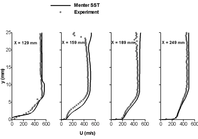
layer characteristics. More recently, Lee et al. [45-46] and Shinn et al. [52] have modeled shock / boundary-layer interactions with micro VG control using structured/ unstructured body-fitted grids with RANS and LES methods. Several experimental investigations of micro VG control of oblique shock / boundary-layer interactions are underway worldwide, but possibly the most complete set of published experimental data is that collected at Cambridge University by Dr. Holger Babinsky and co-workers [37-39]. These experiments use Schlieren imaging, surface oil-flow measurements, Pitot-pressure surveys, and non-intrusive laser Doppler anemometry (LDA) to arrive at a detailed characterization of the effects of micro VGs on boundary-layer properties with and without shock interactions. In this work, a part of the data collected at Cambridge has been used to validate the proposed IB method [Chapter 6].

and that local pressure differences can lead to periodic blowing / suction even in “active” control devices [42], it appears that accounting for the time-dependent nature of the control approach and its interaction with the flow may be critical to achieving better predictions. The geometric complexity of bleed systems complicates the application of techniques such as LES, as resolution of features such as individual holes would normally require a large number of clustered mesh cells. The number of mesh points used could become excessively large, and the accuracy of the LES approach could diminish due to the presence of large numbers of irregular mesh cells. The immersed-boundary method used here makes the simulation of flow problems involving boundary layer suction through a large array of bleed-holes possible, even with sophisticated hybrid LES/RANS turbulence models. Experiments conducted at NASA Glenn Research Center involving boundary-layer flow over perforated plates [62] and shock / boundary-layer interactions with and without active bleed [63] are simulated as part of this work to assess the methodology [Chapter 7].

impingement. The design and evaluation of mesoflap systems have been almost entirely experimental [64-66, 68] with some quasi-steady numerical simulations [44, 67] performed. Gefroh et al. [66] present details of the evolution of the mesoflap designs, which shows that development in design has resulted in shorter mesoflaps and wider gaps. In their work, Wood et al. [67] solved a fluid-structure interaction problem for the flow-control simulation of an (impinging shock) SBLI by adopting a loosely coupled approach, with finite-element modeling for both the structural (mesoflaps) and fluid solvers. A RANS turbulence closure was used in this case [67]. In this work, experiments conducted at University of Illinois at Urbana-Champaign involving SBLI with and without a mesoflap system [65] are used to assess the ability of the immersed-boundary method (proposed in this work) in simulating flow effects induced by moving devices [Chapter 8].

Chapter 2

Governing Equations

The governing equations for compressible viscous fluid flow are the Navier-Stokes equations which can be expressed using tensor notation as

0 = ¶ ¶ + ¶ ¶ j j x u t r r (2.1)

i j ij

i

j i j

uu t

u p

t x x x

r

r ¶ ¶

¶ ¶

+ = - +

¶ ¶ ¶ ¶ (2.2)

2 2

i i i i

j j ji i

j j

u u u u

e u h q t u

t r x r x

é ù é ù

¶ æ ₊ ö ₊ ¶ æ ₊ ö _{= -} ¶ _{é - ù}

ç ÷ ç ÷

ê ú ê ú ë û

¶ ë è øû ¶ ë è øû ¶ (2.3)

where the viscous stress tensor, t_ij, is given by

2 2

3

ij ij ij kk

t =mæ_ç S - d S ö_÷

è ø (2.4)

where, 1

2 j i ij j i u u S x x æ_¶ ¶ ö = ç_ç + ÷_÷ ¶ ¶

is the strain rate tensor. The internal energy e and enthalpy h per unit mass, and the heat flux q_iare defined as,

v

e C T= (2.6)

p

h C T= (2.7)

Pr

P i

i

C T

q

x

m ¶

=

¶ (2.8)

where molecular viscosity μ can be determined using Sutherland’s Law [69] and the assumption of a calorically perfect gas result in constant values ofC_pand C_v.

The system is closed with the assumption of a constant Prandtl number (Pr), and the equation of state for an ideal gas which is,

p=rRT (2.9)

steps/intervals should be very small. This requires huge amount of computer memory and computational time [69] which can be very expensive if feasible. In general, for turbulent flows, the flow solver does not discretize and solve these equations but a set of time averaged as in Reynolds-averaged Navier-Stokes) or spatially filtered (as in Large Eddy Simulation) equations.

2.1 Time Averaging: Reynolds-Averaged Navier-Stokes (RANS)

Equations

The most commonly used temporal averaging technique used is the Reynolds averaging which is defined for any flow property xas,

( )

ò

º x

x 1 (2.10)

To employ Reynolds averaging for the fluid flow equations, any instantaneous flow property is split into a time averaged quantity plus some fluctuation, a process which is known as Reynolds decomposition [69]

x x x= + ¢ (2.11)

Application of the averaging procedure leads to the corollary/fact that the time average of the fluctuation is equal to zero, i.e. x¢ =0

( )

( )

rx r

x r

x º =

ò

ò

Similar to the Reynolds decomposition, any instantaneous flow variable can be decomposed into a Favre averaged and a fluctuating component,

x x

x = ~+ ¢¢ (2.13)

However, unlike in Reynolds averaging, the time average of the fluctuating part is not equal to zero in this case. To perform the time-averaging of the compressible Navier-Stokes equation, the decomposition used for the variables is as follows [69],

T T T p P p w w w v v v u u u ¢¢ + = ¢ + = ¢¢ + = ¢¢ + = ¢¢ + = ¢¢ + = ~ ~ ~ ~ r r r (2.14)

The Favre averaged mean mass, momentum and energy equations for compressible flow are given below, 0 ~ = ¶ ¶ + ¶ ¶ i i x u t r r (2.15)

(

)

j i j

j i

i _{t uu}

x x P x u u t

u~ r~~ _r~~

(

)

2 2 2 2

2

i i i i i i i i

j j

j

j i i i ij i j j j ji i

j j

u u u u u u u u

e u h u

t x

u u u

u t u u q h u t u

x x r r r r r r r é ¢¢ ¢¢ù é ¢¢ ¢¢ù ¶ æ ₊ ö_{+ +} ¶ æ ₊ ö_{+ =} ê ç ÷ ú ê ç ÷ ú ¶ _ë è ø _û ¶ _ë è ø _û é ¢¢ ¢¢ ¢¢ù ¶ _{é - ¢¢ ¢¢ ù+} ¶ _{- - ¢¢ ¢¢+ ¢¢+} ê ú ë û ¶ _{¶ êë úû} % % _% % % % % % % (2.17)

2 3

j i

ij i j T ij

j i

u u

u u k

x x

rt = -r ¢¢ ¢¢=m æç_ç¶ +¶ ö÷_÷- r d

¶ ¶

è ø (2.18)

where rkis the Favre averaged turbulent kinetic energy per unit volume and is defined as,

1 2 i i

k u u

r = r ¢¢ ¢¢ (2.19)

The term 2

3r dk ij in Equation (2.18) is usually ignored in zero-equation turbulence

models and is also ignored here. A zero equation model is one in which no additional transport equations are derived. Similarly, if for any turbulence model transport equations are developed for one quantity, for example the turbulent kinetic energy, the turbulence model is classified as a one equation model and so on. For models involving a turbulent kinetic energy transport equation,rk is solved for. The parameter m_T introduced in Equation (2.18), is modeled in different ways based on the type of turbulence model used. The quantity rh u¢¢ ¢¢ which is defined as the turbulent heat flux q_Tj is modeled as,

Pr

T Tj

T j

T

q h u

x m

r ¢¢ ¢¢ ¶

= =

-¶ (2.20)

diffusion term,t u_{ji i}¢¢, and the turbulent transport term 2

j i i

u u u r ¢¢ ¢¢ ¢¢

. These terms are ignored for

any zero-equation model and sometimes also for the higher equation models.

Considering these simplifications, the Favre-averaged mean equations can be written in compact form as,

0 ~ = ¶ ¶ + ¶ ¶ i i x u t r r (2.21)

(

)

j i j

u u

u P

t

t x x x

r

r ¶ _rt

¶ ¶ ¶

+ = - +

-¶ ¶ ¶ ¶

% %

% _(2.22)

(

)

j i ij ij j Tj ji i

j j j

u u u

E u H u t q q t u

t x x x

r

r r rt é ¢¢ ¢¢ ¢¢ù

¶ _{é ù+} ¶ _{é ù=} ¶ _{é + ù+} ¶ _{- - + ¢¢+}

ê ú

ë û ë û ë û

¶ % ¶ % % ¶ % _{¶ êë} % _úû (2.23)

where E%and H% are the total energy and enthalpy, per unit mass, and given by

2

i i

u u

E e% %= + % % and

2

i i

u u

H% = +h% % % (2.24)

2.2 Menter k-

ω

/ k-

ε

Model

Menter’s model is a two equation turbulence model [72], which is a combination of the

k-ω model [69] and the k-ε model. In this, the k-ω model is used in the near wall region, where it can be used all the way to the wall through the viscous sub-layer, and the k-ε model is used in the outer part of the boundary-layer region. The use of the k-ε model in the outer part of the boundary layer is needed as the k-ω model has been shown to be sensitive to freestream conditions [73]. The two equation Menter model in conservative form is given as,

( )

(

)

₍

₎

ij k T

j j j j

ku

k u k

k

t x x x x

r r

t b r w m s m

¶ é ù

¶ _{+ =} ¶ _{- +} ¶ ₊ ¶

ê ú

¶ ¶ ¶ ¶ _êë ¶ _úû (2.25)

( )

(

)

₍

₎

(

)

j T j j j

j j

u _u

t x x x x

k F

x x

r

r g _{b rw m s m}

n

rs w

w

w

w2

¶ w é ù

¶ w ¶ ¶ ¶w

+ = - + ê + ú ¶ ¶ ¶ ¶ _êë ¶ _úû ¶ ¶ + -¶ -¶ (2.26)

In the above equations, F₁ is a blending function which is used to combine the k-ω model and transformed k-ε model [72] and is given by,

( )

1 1

2

1 2 2

tanh arg

4 500

arg min max ; ;

0.09 _kw

F

k k

y y CD y

w rs n w w = é æ ö ù = ê ç_ç ÷_÷ ú ê è ø ú ë û (2.27)

where, y is the distance from the nearest surface and the term CD_kw is given by,

20

max 2 ,10

kw j j k CD x x rs w w -w2 æ _{¶ ¶} ö = ç_ç ÷_÷ ¶ ¶

The blending function in Equation (2.27) was designed to have a value of one in the near-wall region and zero away from the surface. In Equations(2.25-2.28),_b*_,

k

s , g , b, s_w, s_w2 are model constants which can be found in [72]. The eddy viscosity for the BSL model is given by , T BSL k n w = (2.29)

The equations for the Menter SST model are the same as those for the Menter BSL model, but the values of the constants are different [72]. However, the primary change for the Menter SST [72] model is in the definition of the eddy viscosity,

(

)

, 1 2 max ; T SST a k a F n w = W (2.30)

where, a₁ is a constant, W is the absolute value of the vorticity, and F₂ is a blending function given by,

( )

2 2

2 2

tanh arg

500

arg max ;

0.09 F k y y n w w = æ ö = ç_ç ÷_÷ è ø (2.31)

2.3 Large Eddy Simulation

In the case of spatial averaging as used for LES methods, a filtered flow quantity is obtained by a filtering operation as shown here,

where the integration is performed over the entire flow domain and G

( )

( )

( )

ò

(2.33)

Any flow variable xcan thus be decomposed into a filtered component and a residual part. The application of the filtering process on the Navier Stokes equations result in filtered set of equations which is similar to the time-averaged equations presented earlier and is shown here in a compact form.

0 ˆ ˆ = ¶ ¶ + ¶ ¶ i i x u t ) r r (2.34)

(

)

ji j i j j i i _t x x P x u u t

u r _t

r -¶ ¶ + ¶ ¶ -= ¶ ¶ + ¶ ¶ˆ) ˆ)) _ˆ (2.35)

( )

₍

₎

₍

_{) (}

₎

ˆ SGS SGS

j j ij ij j j

j j

e

hu u t q q

t x x

r r t ¶ ¶ _{¶ é ù} + = _ë + - + _û ¶ ¶ ¶ ) _{)) ) ) )} (2.36)

The total energy and total enthalpy per unit mass are defined as

1 2

v i i

e C T)º )+ u u) ) (2.37)

1 2

p i i

where k is a measure of the sub-grid scale kinetic energy defined as

»

1

( )

2 i i i i

k= u u -u u) ) (2.39)

The filtered viscous stress t)_ij is given by,

( )

ij ij

t) =m T) s (2.40)

where, 2 3 j i k ij ij

j i k

u

u u

x x x

s = ¶ +¶ - d ¶

¶ ¶ ¶

)

) )

(2.41)

The sub-grid scale stress and heat flux are defined as,

¼

(

)

ˆ

SGS

ij u ui j u ui j

t º -r -) ) (2.42)

»

(

)

ˆ

SGS

j j j

q º -r Tu T u- ) ) (2.43)

The sub-grid scale stresses SGS ij

t and heat flux SGS j

q cannot be directly evaluated but need to modeled. A common approach is to employ a subgrid scale (SGS) eddy-viscosity model, and using such an approach, the terms are modeled in this work as,

,

SGS

ij T i j

Pr p SGS j T t j C T q x m ¶ = -¶ ) (2.45)

where m_Tis the eddy viscosity and Pr_t= 0.9 for turbulent flows. In this work a hybrid (LES/RANS) turbulence model has been used, and the eddy-viscosity m_T for the LES part of hybrid model is obtained using the mixed-scale model due to Leonormand et al. [74].

2.5 Mixed Scale Model

The subgrid scale eddy viscosity of the LES part of the hybrid LES/RANS model (outlined in next section) used here is based on the mixed scale model due to Leonormand et al [74]. The sub-grid eddy viscosity for this model [74] is given as,

1 2

2 1/ 2 2 1/ 4 3/ 2

,

2

( ) , 0.06 and

3

j

i i i i

T M M M

j i j j i

u

u u u u

C S q C S

x x x x x

n = D = =éê¶ ¶ +¶ ¶ _{- ç}æ¶ ö_÷ úù

¶ ¶ ¶ ¶ ¶

ê è ø ú

ë û

%

% % % % _(2.46)

whereD = D D D3 _{x y zis a filter width. An estimate of the subgrid kinetic energy q}2_{, is}

obtained from the equation,

2 1₍ ˆ ₎2

2 k k

q = u% %-u (2.47)

where ˆu%_kis a filtered velocity obtained by test-filtering the resolved-scale velocity datau%_k. A box type filter is used for the test filtering.

2.6 Hybrid LES/RANS Methodology

BSL model is used as the RANS component of the hybrid LES/RANS model, as previous studies [9, 75] have found that this approach provides generally better results than the use of the SST model.

The hybrid LES/RANS model used in the present study [75] only involves modifications to the eddy viscosity description, which is given by,

(

)

t t T BSL T M

m =rn =r nG + - Gn (2.48)

where Gis a blending function. As the blending function Gapproaches one, the closure approaches its RANS (Menter BSL) description, and as it approaches zero, a subgrid eddy viscosity is obtained. The blending function Gis based on the ratio of the wall distance d to a modeled form of the Taylor micro-scale:

2

1

1 tanh[5( 1) ) ,

2

d Cm

k

h f h

ac

æ ö

ç ÷

G = - - + =

ç ÷

è ø

(2.49)

where f is set to tanh-1(0.98) _{in order to fix the balancing position (where}

m

kh2 = C _{) to}

inflow. This is done using Coles’ law of the wall/wake in conjunction with van Driest transformation:

( )

1

ln 2 sin ,

2 vd w w w u d u d

d C d

u

t

t

p

k k d n

+ P æ ö +

= + + _{ç ÷} =

è ø (2.50)

An estimate of the outer extent of the log-layer is made by determining the value ofd_w+such that,

( )

ln vd 0.98

w u d C u_t k + æ ö æ ₊ ö ₌ ç ÷ ç ÷

è _{ø è} ø (2.51)

The value of d u dt

n

+ _{= that correspond to this value of}

w

d+ _{needs to be determined next which}

is dependent on the variation of the kinematic viscosity in the boundary layer and hence on the distribution of static temperature within the boundary layer. The static temperature distribution within the boundary layer is obtained using Walz’s relationship given by,

(

)

(

)

2

1 2

aw w w T T

T

T u u

r M

T T T u u

g

¥

¥ ¥ ¥ ¥ ¥

- - æ ö

= + - _{ç ÷}

è ø (2.52)

The model constant is then determined by equating d+to _a2 _{which is based on the inner}

Table 2.1 Model constant a

( )

Case a

( )

Vortex generator simulations [Chapter 6] _{27.35 39.02+ x-19.21x}2

Bleed-hole array simulations [Chapter 7] 53.90 11.04+ x

Mesoflap simulations [Chapter 8] 38.46 49.78+ x

Chapter 3

Numerical Methods

3.1 Discretization of Fluxes

A finite volume method of discretization has been used for the fluid solver in the work presented here. In a finite volume approach, the value of the flow variable is solved at the geometric center of the cell and not at the nodes. The integral or conservation form of the governing equations for a control volume V is given as follows,

( )

CV dV CS dA CV dV

t

¶ _{+ =}

¶

Ó

òòò

Ò

òò

Ó

òòò

u v w E k r r r r r r rw é ù ê ú ê ú ê ú ê ú = ê ú ê ú ê ú ê ú ê _úû ë U (3.2)

Although no over bar or tilde is used for the flow variables in the above equation, the variables are either time-averaged (RANS) or filtered (LES). Integrating Equation (3.1) over the control volume in computational space results in a semi-discretized conservation equation which can be written as,

, ,

1/ 2, , 1/ 2, , , 1/ 2, , 1/ 2, , , 1/ 2 , , 1/ 2 , ,

i j k

CV i j k i j k i j k i j k i j k i j k i j k CV

V V

t - + - + - +

¶

+ + + + + + =

¶ U

E E F F G G S (3.3)

For a structured domain, as is used in this work, the flux vectors E, F, G are at the cell faces in the ‘i’, ‘j’, ‘k’ direction respectively. The residual vector R_{i j k, ,} at any point is given by,

, , 1/ 2, , 1/ 2, , , 1/ 2, , 1/ 2, , , 1/ 2 , , 1/ 2 , ,

i j k = i- j k+ i+ j k+ i j- k + i j+ k+ i j k- + i j k+ - i j k CVV

R E E F F G G S (3.4)

3.2 LDFSS

LDFSS is a method of flux splitting which is based on the van Leer method of flux splitting [78]. In this method, the inviscid flux is conveniently split into a convective part and a pressure part. The convective part is dependent on the wave speeds at the cell interfaces and requires the calculation of interface Mach numbers. This is in consideration of the hyperbolic nature of the convection process. Thus the inviscid flux at any face of a cell, for instance the ‘i+1/2’ face, can be expressed as,

(

)

1/ 2 1/ 2 1/ 2 1/ 2

c p

i+ =Ai+ run i+ + p i+

E E E (3.5)

where c

n

u

r E is the convective flux, p_Ep _{is the pressure flux (both per unit area), and} n

u is the velocity normal to the cell face. The subscripts ‘j’ and ‘k’ have been dropped here for convenience. Equations (3.6) and (3.7) give the convective and pressure components, _Ec_and

0 0 0 0 x y p z n n n é ù ê ú ê ú ê ú ê ú = ê ú ê ú ê ú ê ú ê ú û ë E (3.7)

The normal velocity at the cell face, u_n is calculated by using the equation,

n x y z

u =un +vn +wn (3.8)

where n_x, n_y, n_z are the components of the unit normal vector at the cell face. The convective flux at the interface is constructed as

(

)

1/ 2 1/ 2

c L c R c

n L R

u a C C

r _{E =} r +_{E +}r -_{E (3.9)}

where the subscript ‘i’ has also been omitted for simplicity of notation. Here the suffixes ‘L’ and ‘R’ denote the fluxes at left and right neighbors of the interface (first order), and a_{1/ 2}is an interface speed of sound which is defined as,

(

)

1/ 2

1

2 L R

a = a +a (3.10)

The coefficients C-and C+are based on the van Leer coefficients C_VL-and C_VL+

respectively,

1/ 2

VL

C+ =C +-M+ (3.11)

1/ 2

VL

(

)

VL L L L L L

C+ =a+ +b M -b M (3.13)

(

)

VL R R R R R

C- ₌a- ₊b M _-b M _(3.14)

1/ 2 1/ 2

2 R L R

R L L

p p

p

M M

p p d p

+ ₌ æ _- - ö

ç ₊ ÷

è ø (3.15)

1/ 2 1/ 2

2 L L R

R L R

p p

p

M M

p p d p

+ ₌ æ _- - ö

ç ₊ ÷

è ø (3.16)

(

)

, max 0.0,1.0 int ,

L R ML R

b = - é_ë - ù_û (3.17)

(

)

, ,

1

1 sign 2

L R ML R

a± _{= é + ù}

ë û (3.18)

In Equations (3.15) and (3.16) the term d is a weighting parameter [77] which is generally set to unity. The terms M_{1/ 2} and p_{L R,} are given by,

(

)

1/ 2 1 1.0 4 2 L R L R

M = b b æ_çç M +M - ö_÷÷

è ø (3.19)

(

) (

)

, , ,

1

1 2

4

L R L R L R

p± = ±M _mM (3.20)

In Equation (3.17), the function ‘int’ returns the integer part of the value passed to it, and in Equation (3.18), the function ‘sign’ returns a value of 1 for positive arguments and -1 for negative arguments. This makesbL R, vanish if the flow is supersonic and behave like a sonic

switch. The left and right state Mach numbers are given as follows,

, , ,

,

1 2

x L R y L R z L R L R

n u n v n w

M

a

+ +

As shown in the preceding section, the calculation of the interface flux depends on the determination of the left (L) and right (R) states. For a first order reconstruction, ‘L’ and ‘R’ denote the fluxes at left and right neighbors of the interface. To achieve greater accuracy in computations the inviscid flux reconstruction is needed to be made second or higher order and this is done here using the Piecewise Parabolic Method (PPM) due to Colella and Woodward [79]. The implementation of this method in its baseline form has been outlined in [13] and is shown here. In the PPM method, the flux at any interface is first expressed as a function of the primitive variable vector, V=

[

]

1/ 2 1/ 2( , 1/ 2, , 1/ 2)

i+ = i+ L i+ R i+

F F V V (3.22)

where,

(

)

(

)

, 1/ 2 , 1/ 2 1 2 1

7 1

12 12

L i+ = R i+ = i+ i+ - i+ + i

-V V V V V V (3.23)

for sufficiently smooth data. A condition is imposed such that the left and right states are set equal to the value at the cell center if a local extrema is detected. Thus,

(

)(

)

, 1/ 2 , 1/ 2

if sgn _{L i i i R i} 1, then

L i R i i

+

-+

-é - - ù=

-ë û

= =

V V V V

V V V (3.24)

(

)(

)

(

)

(

)

(

)

, 1/ 2 , 1/ 2

, 1/ 2 , 1/ 2 , 1/ 2 , 1/ 2 , 1/ 2 , 1/ 2

, 1/ 2 , 1/ 2

if sgn 1, then

1

; 6

2

if then 3 2

if then 3 2

L i i i R i

L i R i i L i R i

R i i L i L i i R i

C D DC CC CC DC + -+ - + -- + + -é - - ù¹ -ë û é ù = - = _ê - + _ú ë û

> =

-- < =

-V V V V

V V V V V

V V V

V V V

(3.25)

This check resets the value at the interface (right or left depending on the shape of the parabola) of the cell such that the interpolation parabola is a monotone.

3.3 Time Integration

Second order temporal accuracy is achieved using a Crank-Nicholson time discretization. The Crank-Nicholson discretization leads to the formation of a residual vector which can be expressed as,

(

) ( )

1,

1, 1 1 1,

2

n k n

n k n k n

t + + + ₌ - _{+ é} + _{+ ù} ë û D U U

R R U R U (3.26)

where the suffix ‘n’ denotes the time step or iteration level and ‘k’ is a sub-iteration index. A planar relaxation scheme is used to solve the system of linearized equations at each sub-iteration [80]. The number of sub-sub-iterations required is based on achieving a specified level of convergence at each time step. This is measured by the relative drop of the norm of the residual, such that if the iteration converges after ‘l’ sub-iterations, then it should satisfy the condition,

1, 1, 1

n k l n k tol

+ =

+ = <

R

R (3.27)

3.4 LES/RANS: Initialization

The LES/RANS simulations were initialized by superimposing scaled fluctuations from a previous 3-D LES computation, henceforward referred to as database, onto a converged RANS flat plate calculation. The RANS calculations were done as a 2-D flat plate simulation using the experimental free stream and wall (isothermal or adiabatic) conditions. A separate flat plate simulation was thus done for each experiment simulated and the fluctuations for the velocity components were scaled for the different simulations as follows,

, , , , , , RANS scaled data data RANS scaled data data RANS scaled data data u u u u u v v u u w w u t t t t t t ¢ = ¢ ¢ = ¢ ¢ = ¢ (3.28)

In the above equation, the subscript ‘data’ corresponds to the database and the subscript ‘RANS’ refers to the 2-D flat-plate simulation. A scaling is also performed to obtain the x, y and z locations in the domain for the LES/RANS simulation which correspond to grid points (where the fluctuations are stored) in the domain for the database. This is given by,

With the scaled locations and fluctuations computed, the resulting initial values of the primitive variables ρ, u, v, w, T, at any point in the computational domain (for the LES/RANS simulation), are obtained as

2 2 2

0, 1 2 1 RANS scaled RANS scaled RANS scaled RANS RANS

u u u

v v v

w w w

u v w

T T R p RT g g r ¢ = + ¢ = + ¢ = + + + = -= (3.30)

where, T_0,RANS is the stagnation temperature obtained from the RANS computation.

3.5 LES/RANS Inflow Generation: Recycling/Rescaling

plane by matching the a) wall co-ordinates given by d_w+_{, which correspond to an inner-layer}

scaling and b) h y

d

= values which correspond to an outer layer scaling. This procedure

results in two sets of fluctuating values given by,

( )

inn rec _inl

q¢ =q¢ é_ë u y_t ù_û (3.31)

out out inl y q q d é_{æ ö} ù ¢ = ¢ _{êç ÷ ú} è ø

ë û (3.32)

where the suffixes ‘inn’ and ‘out’ refer to the inner and outer boundary-layer scaling respectively. These set of values are then combined to get q_rec¢ using a blending function which is given by,

(

)

rec inn out

q¢ = -W q¢ +Wq¢ (3.33)

( )

₍

(

₎

)

2 tanh 4 1 2

B W B B h h h æ ì_ï é - ùü_ï ö ç ÷ = _í + _{ê úý} ç _{ïî êë} - + _úûïþ ÷ è ø (3.34)

where B is the value of h y

d

= where the boundary layer transitions from the inner to the

outer layer and is set equal to 0.2 in this work. The rescaled value of the turbulence variables

[k, w, Γ] are obtained in a similar fashion as in Equation (3.33) with the actual value of the

(

)

, primitive variables

in RANS Kleb rec

q =q + G q¢ (3.35)

(

)

, turbulence variables

in RANS Kleb rec

q =q + G q (3.36)

In the Equations (3.35) and (3.36) the function G_Kleb is a Klebanoff type intermittency function [69] given by,

1 6

( ) 1 inl

Kleb

Kleb inl

y y

C d

-æ _{æ ö} ö

ç ÷

G _{= + ç ÷}

ç _{è ø} ÷

è ø

(3.37)

Chapter 4

Immersed Boundary Methodology

The immersed boundary (IB) method used here is an extension of the method developed by Choi et al. [35] (at NC State) for 3-D incompressible flows. This belongs to the class of IB methods based on the direct forcing technique proposed by Fadlun et al. [25]. The primary concept adopted in this approach is that the velocity of the fluid should be equal to the velocity of the moving body at its surface. This is achieved by use of a forcing approach in a discrete sense in which the flow in the vicinity of the immersed surface is reconstructed [17, 24-25, 30, 33] by use of interpolation functions. This is done in a way which ensures that the boundary velocity is recovered as the solution at each time step for a time-dependant simulation. In this work, this original approach has been augmented and somewhat modified for use in compressible flows [82].

4.1 Cell Classification

closed surface) and interior cells which are inside the immersed object. Figure 4.1 shows a schematic of the cell classification. The classification is based on a signed distance function which gives the distance of any computational node from its nearest surface point and is derived from concepts of computational geometry. The sign associated with the distance indicates whether the node is inside or outside the immersed body. The first step is to render the immersed surface as a set of points (which may or may not be structured) with their surface normal provided. The immersed surface can be rendered as more than one level set depending on the complexity of the problem.

This becomes very useful for an object which might have different motion patterns in different parts of its surface as in the case of a walking human body. The rendition can be

Fig. 4.1 Cell classification scheme for immersed boundary method Field points Band points Interior points

Immersed body surface

Interior points Field points