SRIVASTAVA, MANU. Image Processing and Analysis of Vapor Bubbles nucleated in Thin Liquid Film Boiling. (Under the direction of Dr. Nam T. Dinh and Dr. Tiegang Fang).
This study is concerned with physics of high heat-flux boiling that governs Critical Heat Flux (CHF) upon Departure from Nucleate Boiling (DNB). The focus is placed on nucleation pattern, dynamics and interactions of vapor bubbles in a micro-layer. An
Autonomous Image Processing Tool is developed to extract bubble characteristics from high speed video (10000fps) of high heat flux (836, 1118, 1504 and 1893 kW/m2), thin-film boiling of water over a horizontal surface (Ti36Sb dataset, BETA-B experiment).
Advanced image processing techniques involving noise removal, thresholding and segmentation operations are applied for processing each image frame. A multilayer
perceptron neural network, trained on 20ms of manually identified bubble data, is used for autonomous bubble identification with an accuracy of 70-80%. After tracking individual bubbles over 60ms, bubble characteristics such as maximum base area, residence time and expansion velocity are calculated.
Statistical analysis of bubble characteristics reveals their growth patterns. It was observed for the first time that bubble bases expand in an accelerating manner with time. This behavior is explained by the distribution of superheat of fluid in the vicinity of
nucleating bubbles. Notably, the bubble base expansion velocity is found to increase with the imposed heat flux.
Another observation was that the surface averaged bubble base expansion velocity of bubbles nucleated from high frequency nucleation sites is larger than that ofbubbles
growth, statistical analysis of bubble characteristics and spatial analysis of spatio-temporal pattern have not exhibited a critical behavior postulated to occur at CHF.
by
Manu Srivastava
A thesis submitted to the Graduate Faculty of North Carolina State University
in partial fulfillment of the requirements for the degree of
Master of Science
Mechanical Engineering
Raleigh, North Carolina 2015
APPROVED BY:
_______________________________ _______________________________ Dr. Nam Dinh Dr. Tiegang Fang
Committee Co-Chair Committee Co-Chair
_______________________________ Dr. Alexei Saveliev
DEDICATION
BIOGRAPHY
ACKNOWLEDGMENTS
I thank my advisor, Dr. Nam Dinh, for his unwavering support. His guidance at every step of the way was invaluable. I also thank Dr. Joel Trussell for his guidance during work on neural networks. I am also thankful to Dr. Tiegang Fang for the providing support when needed.
TABLE OF CONTENTS
LIST OF TABLES ... vii
LIST OF FIGURES ... viii
1 LITERATURE REVIEW ... 1
1.1 Introduction ... 1
1.1.1 The Boiling Curve ... 1
1.1.2 CHF ... 2
1.1.3 Criticisms of Hydrodynamic models and Recommendations ... 4
1.2 BETA Experiments ... 6
1.2.1 Overview of BETA-A Results ... 8
1.2.2 Overview of BETA-B Results ... 8
1.3 Scale Separation Phenomenon ... 11
1.4 Research Objectives ... 14
1.5 Summary ... 16
2 BETA-B EXPERIMENT: DESCRIPTION AND DATA ... 18
2.1 Description ... 18
2.2 Data ... 20
2.2.1 Features of Interacting Bubbles in visual data of Ti36SB... 21
2.3 Image Processing Challenges ... 24
2.4 Methods for Data Analysis ... 25
2.5 Summary ... 26
3 IMAGE PROCESSING ... 27
3.1 Algorithm ... 27
3.2 Image Segmentation ... 27
3.2.1 Thresholding: Grayscale - Binary Conversion... 28
3.2.2 Marker Based Watershed Segmentation ... 30
3.3 Neural Networks for Bubble Identification ... 31
3.3.1 Neural Network Architecture ... 31
3.3.3 Neural Network Training ... 32
3.3.4 Neural Network Output Vector ... 34
3.3.5 Forward Relaxation ... 34
3.4 Tracking ... 34
3.5 Quantification of bubble detection accuracy ... 37
3.6 Sources of Errors ... 40
3.6.1 Grayscale to Binary Thresholding ... 40
3.6.2 Watershed Segmentation... 40
3.6.3 Neural Network Bubble Identification... 40
3.7 Summary ... 41
4 DATA ANALYSIS AND RESULTS ... 42
4.1 Primary Analysis ... 42
4.1.1 Active Nucleation Site Density (NSD) ... 42
4.1.2 Minimum Nucleation Distance ... 46
4.1.3 Nucleation Rate ... 48
4.1.4 Residence Time (tres) ... 50
4.1.5 Maximum Bubble Area ... 52
4.1.6 Area Expansion Velocity ... 53
4.1.7 Average Instantaneous Expansion Velocity ... 55
4.2 Secondary Analysis ... 56
4.2.1 Identification of High Frequency Nucleation Site Cluster ... 57
4.2.2 Spatial Analysis of Pattern ... 61
4.3 Errors, Biases and Uncertainty in Data Analysis ... 70
4.4 Summary ... 72
4.4.1 Key Speculations ... 75
4.4.2 Key Assumptions ... 75
5 CONCLUSIONS ... 76
REFERENCES ...80
LIST OF TABLES
Table 1 Observations from primary analysis... 72
Table 2 Observations from secondary analysis ... 74
Table 3 Key speculations ... 75
LIST OF FIGURES
Figure 1 Boiling curve ... 1
Figure 2 Photograph taken from below of Carbon tetrachloride boiling on horizontal glass plate (Nelson, 2001) ... 5
Figure 3 Schematic of the BETA experiment in two configurations (Theofanous, et al., 2002) ... 7
Figure 4 Bubble diameters as function of time for BETA B experiment. (Liu, et al., 2014) .... 9
Figure 5 Burnout caused by long lasting bubble (Theofanous, et al., 2002) ... 10
Figure 6 Experimental evidence of scale separation (Theofanous, et al., 2002) ... 12
Figure 7 Regular behavior of nucleation site shown by infrared images, (Theofanous, et al., 2002) ... 12
Figure 8 Schematic of scale separation concept (Theofanous, et al., 2002) ... 13
Figure 9 Schematic of the BETA experiment in two configurations (Theofanous, et al., 2002) ... 19
Figure 10 SEM images (50000x magnification) of heaters well-aged by pulse heating over a long period (12 hours) at 200°C. The time-to-burnout from the heater installation in to test section was 36-48 hours. The measured CHF in well-aged heaters were 2.0-3.0 MW/m2 (Dinh & Tu, 2007)... 20
Figure 11 Synchronized sequence of video and IR images for Run Ti30SA_II04, 1500 kW/m2. The IR image (right column) shows dark (low temperature) spots as footprints of bubbles (Dinh & Tu, 2007)... 21
Figure 12 The BETA-B video image of an evaporating liquid film at a high heat-flux. Time interval between consecutive images ~0.09 ms (Ti36SB07, 1893 kW/m2). (Dinh & Tu, 2007) ... 22
Figure 13 A close-up view of the bubble collapse and liquid return to the bubble base. Time interval between consecutive images 0.18 ms (Ti36SB07, 1893 kW/m2). The thickness of the liquid layer is estimated to be more than 100 μm (Dinh & Tu, 2007) ... 23
Figure 14 Nucleation of a bubble in the vicinity helps to remove the “stubborn” bubble. Time interval between consecutive images 0.09ms (Ti36SB07, 1893 kW/m2). (Dinh & Tu, 2007) . 24 Figure 15 Original BETA-B image (L) and binary image (R) obtained after Step 1: Segmentation ... 27
Figure 16 Image segmentation ... 28
Figure 17 Opening-closing with (R) and without (L) morphological reconstruction ... 29
Figure 18 Before (L) and after (R) watershed segmentation ... 30
Figure 19 Image processing from start to end. Input image (L), reconstructed image (C L), thresholded image (C R), after marker based watershed segmentation (R) ... 30
Figure 20 Used neural network architecture... 31
Figure 21 Neural network training (L) (Hagan, et al., 2002) and our case (R)... 33
Figure 22 Trained neural net in action... 33
Figure 23 Bubble tracking flowchart ... 35
Figure 25 Frames 315-316 ... 38
Figure 26 Frames 317-318 ... 39
Figure 27 Frames 319-320 ... 39
Figure 28 Active NSD = 3 (assuming area = 1m2) ... 42
Figure 29 Distribution of active NSD – lower heat fluxes, 621 samples each ... 43
Figure 30 Distribution of active NSD - higher heat fluxes, 621 samples each ... 43
Figure 31 Mean and mode of active NSD at all fluxes ... 44
Figure 32 Distribution of active NSD in Central Window (1.9 x 3.7mm2) - lower heat fluxes, 621 samples each ... 45
Figure 33 Distribution of active NSD in Central Window (1.9 x 3.7mm2) - higher heat fluxes, 621 samples each ... 45
Figure 34 Mean & mode of active NSD in Central Window (1.9x3.7mm2) at all heat fluxes 46 Figure 35 d = Minimum nucleation distance ... 46
Figure 36 Distribution of min. nucleation distance - lower heat fluxes, 203 & 292 samples respectively ... 47
Figure 37 Distribution of min. nucleation distance - higher heat fluxes, 319 & 488 samples respectively ... 47
Figure 38 Distribution of bubble nucleation rate - lower heat fluxes ... 48
Figure 39 Distribution of bubble nucleation rate - higher heat fluxes ... 49
Figure 40 Progression of bubble area in sequential frame used to determine bubble residence time ... 50
Figure 41 Distribution of bubble residence time - lower heat fluxes, 220 & 301 samples respectively ... 50
Figure 42 Distribution of bubble residence time - higher heat fluxes, 326 & 490 samples respectively ... 51
Figure 43 Distribution of max bubble area - lower heat fluxes, 220 & 301 samples respectively ... 52
Figure 44 Distribution of max bubble area - higher heat fluxes, 326 & 490 samples respectively ... 52
Figure 45 Distribution of bubble area expansion velocity - lower heat fluxes, 220 & 301 samples respectively... 53
Figure 46 Distribution of bubble area expansion velocity - higher heat fluxes, 326 & 490 samples respectively... 54
Figure 47 Stages of bubble expansion in thin film boiling (Dinh & Tu, 2007) ... 54
Figure 48 Increasing average instantaneous expansion velocity at different heat fluxes ... 56
Figure 49 Variation in distribution of accumulative NSD with heat flux ... 59
Figure 50 Nucleation statistics ... 60
Figure 51 Vapor coverage (L) through nucleation (R) in neighborhood at 1504kW/m2 ... 61
Figure 52 Variation in distribution of bubble DMAX at irregular sites with heat flux ... 62
Figure 53 Variation in distribution of site averaged bubble DMAX at regular sites with heat flux... 63
Figure 55 Variation in the distribution of site averaged bubble tres at regular sites with heat
flux... 65
Figure 56 Variation in the distribution of site averaged tidle at regular sites with heat flux .. 66
1 LITERATURE REVIEW
This chapter provides an introduction to Nucleate Boiling, focusing on the recent changes in its understanding from time and space averaged to a dynamic and asynchronous
phenomenon, the Critical Heat Flux (CHF) and Departure from Nucleate Boiling (DNB).
1.1 Introduction
Nucleate boiling has been studied extensively for the past 60 years. It is an elaborate heat removal mechanism. In nuclear reactors and other high energy density installations where high heat transfer is required within small areas, it is a method of choice. Using single-phase forced convection would be impractical because extremely high bulk velocities would be required.
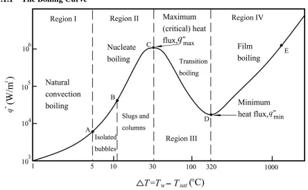
1.1.1 The Boiling Curve
In Figure 1, the ordinate and abscissa denote the heat flux, q”, and surface superheat, ΔT, respectively for pool boiling of water. Nucleate boiling exists between ΔT = 5°C and ΔT = 30°C. The slope represents the heat transfer coefficient, h = q’’ / ΔT. The rapid rise in h is caused by bubble nucleation and enhanced fluid mixing which absorbs heat from the heater surface in the form of latent heat of evaporation and exposes the hotter heater surface to cooler bulk liquid situated above the superheated liquid layer adjacent to the surface. This causes rapid localized cooling for the surface. Increasing the heat flux, increases the number of bubbles and improves the fluid mixing. Thus, only a small increment in surface
temperature is observed for large heat flux increments. This makes nucleate boiling a desirable cooling mechanism for the heater’s surface.
At ΔT approximately equal to 30°C, q’’ reaches its peak. Further increase in heat flux results in Departure from Nucleate Boiling (DNB) or Boiling Crisis. DNB causesdeteriorated heat transfer in film boiling regime, making the heater overheat rapidly to the order of 1000°C. The maximum value of heat flux upon DNB is called the Critical Heat Flux (CHF).
1.1.2 CHF
1.1.2.1 Kutateladze’s Correlation (1952)
Nucleate boiling was considered hydrodynamically similar to gas bubbling through a porous plate used in sieve-tray distillation columns with the gas flow rate analogous to heat flux density. The transition of gas flow from laminar to turbulent (hydrodynamic instability or ‘column flooding’) was considered to represent CHF in boiling. This led to the belief that CHF was purely a hydrodynamic phenomenon and a critical vapor velocity would exist where liquid and vapor would compete for free volume. Using dimensional analysis, Kutateladze derived the widely used CHF correlation:
𝑞′′𝐶𝐻𝐹 = 𝐶𝐻𝐿𝑉[ρ𝑣2 σ g (ρ𝐿 – ρ𝑉)]1/4
1.1.2.2 Zuber’s Hydrodynamic Theory (1959)
Zuber (Zuber, 1959) approached the CHF peak in Figure 1 from the Transition boiling side and analytically derived Kutateladze’s correlation. Transition boiling was understood to be hydrodynamically unstable but with a well-defined geometry, unlike nucleate boiling. He attributed the organization of vapor jets to Taylor instability of a plane interface with the lighter fluid below the heavier fluid and the mushroom clouds in the vapor jets were attributed to Helmholtz instability.
Despite being hydrodynamically unstable, Transition boiling was thermally stable. Since the vapor release process exhibited a periodicity in time, Zuber stated that the maximum
allowable frequency of this system corresponds to the CHF.
𝑀̇ = 𝜌𝑣 𝛱 3
24√2𝛱[
𝜎 𝑚0 𝜌𝑣 ]
1/2
[ 𝜌𝑙 𝜌𝑙+ 𝜌𝑣]
1/2
Where m0 denotes wave number
Evaluating the energy requirement of a vapor column, assuming the surrounding liquid is at saturation temperature,
𝑞′′ = 𝐿𝜌𝑣 𝛱 3
24√2𝛱[
𝜎 𝑚0 𝜌𝑣 ]
1/2
[ 𝜌𝑙 𝜌𝑙+ 𝜌𝑣]
1/2
Where L is the latent heat of evaporation at saturation. The wave number, m0, was determined within the range:
[𝑔(𝜌𝑙− 𝜌𝑣)
𝜎 ]
1 2
> 𝑚0 > [𝑔(𝜌𝑙− 𝜌𝑣)
3𝜎 ]
1 2
Substituting the wave number in the energy equation results in the Kutateladze’s correlation,
𝑞′′
𝐶𝐻𝐹 = 𝑘𝐿[ρ𝑣2 σ g (ρ𝐿 – ρ𝑉)]1/4
1.1.3 Criticisms of Hydrodynamic models and Recommendations
Classical boiling theory and models were based on traditional experiments that assumed a uniform distribution of nucleation site density. Modern experiments with better access to the heater surface revealed that the nucleation site density was spatially non-uniform and the site behavior was dynamic (On at times – Off at times). The traditional view led to a series of predictions that were not observed in modern experiments.
uniform distribution of nucleation site density. The new experiments showed that the heater surface heavily influenced boiling. CHF was found to occur due to the development of dry spots on the heater surface. Also, around the year 2000, a number of experiments also showed that CHF is largely governed by the micro-hydrodynamics of the thin liquid film on the heater surface. On other hand, Zuber’s vapor column instability theory proposed more than half century ago had not been observed in these experiments.
Classical boiling models, based on time and space averaged parameters, “tended to predict lower CHF for higher nucleation site density which is contradicted to the findings of the modern experiments using high-speed infrared imaging for heat-transfer surface thermometry” (Liu, et al., 2014). The newly observed dynamic nature of nucleation sites implied that taking a ‘snapshot’ (as shown in Figure 2) of the heater surface will not reveal the geometric nucleation pattern due to the intermittent behavior of sites. Therefore, the use of averaged parameters precludes the dynamic effects of asynchronous bubble nucleation, growth and departure/collapse processes.
Figure 2 Photograph taken from below of Carbon tetrachloride boiling on horizontal glass plate (Nelson, 2001)
activation. This approach was based on self-organization of boiling. According to him, “Boiling is a structure that results from constrained minimization of temperature peaks of the heater surface (entropy generation minimization). The constraints are placed by the actual distribution of nucleation sites. Its stability results from the geometric optimization process. The system continues to minimize its overall thermal resistance in search for stationary solutions” (Nelson, 2001).
It was established that nucleate boiling (and determination of CHF) should be modeled in a conjugate manner with the heater and more modern boiling experiments that measured local and instantaneous heater surface temperature and observed the micro-hydrodynamics of the thin liquid film were needed.
1.2 BETA Experiments
“New kinds of experiments and visualizations on the micro-hydrodynamics of high heat flux pool boiling and burnout are conducted by professor Theofanous’s group at UCSB
(Theofanous, et al., 2002). These BETA experiments use high-speed video and infrared imaging to visually capture the micro-hydrodynamics of evaporating liquid film that constitute the key physics of burnout. Figure 3 depicts the schematic of the BETA
level, until burnout occurred and the heater was destroyed. Visualization records (1 s duration) were obtained in selected runs (mostly at conditions expected to be near burnout), after a short wait to reach steady state at the new power level. The data acquisition rate was up to 68 kHz and 11 kHz for the video and IR cameras, respectively.” (Liu, et al., 2014)
Figure 3 Schematic of the BETA experiment in two configurations (Theofanous, et al., 2002)
“In BETA experiment, the heater is on top of the substrate producing very uniform heat flux on the surface, which helps reduce data uncertainty and renders very small thermal inertia,
therefore the burnout occurred almost immediately at CHF. The temperature of heater’s surface is observed by high speed infrared imaging of the nano-film heater from below using very strong light source for both configurations, A and B. Detailed bubble behavior is
“BETA experiment provides three types of experiment data: (1) the temperature profile of nucleation site at different time steps, (2) the temperature history at the center of nucleation site, and (3) the history of bubble progression. Types 1 and 2 data were extracted from images taken by the high-speed infrared camera and Type 3 data come from the image taken by high-speed video camera used in Configuration B.” (Liu, et al., 2014)
1.2.1 Overview of BETA-A Results
Based on the void fraction near the heater surface, the BETA-A experiment (2002) established that the search for burnout mechanisms should be focused on the
micro-hydrodynamics of evaporating thin liquid film on heater surface. This led to the discovery of the Scale Separation phenomenon by Theofanous et al., which states that liquid-film boiling performed with liquid supply on the side of a heater should exhibit similar behavior as in pool boiling experiments on the same heater.
The Scale Separation phenomenon formed the basis for BETA-B (2007) series of
experiments: removal of liquid pool above the heater’s liquid film allows visual access to nucleation and bubble dynamics in the evaporating liquid film. BETA-B experiments found that there was very small difference between CHFs in Configurations A and B for similar experiment condition ratifying the scale separation assumption. Gong’s experiments also confirmed that liquid films with various thickness have similar CHF (Gong, et al., 2014).
1.2.2 Overview of BETA-B Results
Visual access to the micro-hydrodynamics of thin liquid film revealed dynamic and
thermal factors causing asynchronous activation of neighboring sites constitute collective
behavior of bubbles.
The following observations from BETA depict collective behavior of bubbles:
1. Figure 4 shows bubble diameters as a function of time taken from images obtained in BETA-B experiment.
Figure 4 Bubble diameters as function of time for BETA B experiment. (Liu, et al., 2014)
2. The reversal of the established CHF-NSD trend was first observed in BETA experiments and has also been attributed to collective behavior of bubbles. “As can be seen in BETA-B tests, bubbles are nucleated and grow asynchronously. Consequently, boiling heat transfer analysis framework using aggregated static NSD tends to overestimate the size and lifetime of surface bubbles. Because simultaneous bubbles are few, they do not easily coalesce as suggested by a NSD based static treatment. This recommends the treatment of bubble nucleation as a dynamic phenomenon.” (Liu, et al., 2014)
3. Another observation of the BETA-B experiment was that long lasting bubbles that were nucleated at high superheat caused burnout as shown in Figure 5.
“The reason that the nucleation site activated at such a high superheat is because its neighboring nucleation sites were constantly activated, which prevent expansion of the hot spot site and thus raise the temperature at that spot. When the hot spot site nucleated, intensive evaporation would quickly drain the micro-layer under the bubble causing rapid temperature rise in the region in contact with vapor. This high temperature would keep a residual bubble at that point and keep the liquid from rewetting that spot.” (Liu, et al., 2014). This is an example of thermal interactions driven collective behavior of nucleation sites determining their activation.
Thus, on one hand, collective behavior of bubbles and nucleation sites may have led to the observed increase in heater resilience to burnout under high NSD, while on the other, it could lead to a spike in the local surface superheat causing burnout.
1.3 Scale Separation Phenomenon
Figure 6 Experimental evidence of scale separation (Theofanous, et al., 2002)
“As implied by the experimental evidence, the main idea of the scale separation assumption is the fact that the two-phase hydrodynamics of the bulk fluid do not directly affect CHF; but it can indirectly influence CHF by affecting the hydrodynamics of thin liquid film (which is believed to be in micrometer-scale). As a result, the pool boiling under high heat flux can be separated into several regimes of different scale: (1) the meter-scale (m-scale) bulk fluid, (2) the millimeter-scale (mm-scale) vapor rich layer which separates bulk fluid and thin liquid film, (3) the micrometer-scale (µm-scale) thin liquid film, and (4) the nanometer-scale (nm-scale) surface properties. The CHF is mainly determined by the hydrodynamics of µm-scale thin liquid film, while the nm-scale surface property can strongly impact the hydrodynamics by impacting the nucleation site density, triple contact line dynamics etc. Also, the m-scale bulk fluid can affect the thin liquid film hydrodynamics by inducing shear and droplet irrigation to the liquid film. The interactive relationships between different scales are illustrated in Figure 8.” (Theofanous, et al., 2002)
“It is necessary to mention that the whole system should be in dynamic equilibrium state, but not steady state. The thin liquid film is constantly evaporating, and the bulk fluid
continuously supplies the liquid film preventing burnout of the heating surface by “droplet irrigation”. One implication of the scale separation concept is that the heater surface and the extended liquid micro-layer on it operate autonomously, that is, without any significant influence of the external hydrodynamics. Subsequently, because the presence of the liquid pool is incidental, the burnout phenomenon can be studied independently by focusing on the micro-layer of the heater system alone.” (Theofanous, et al., 2002)
Therefore, assuming that the scale separation concept holds true, insights into high heat flux pool boiling and the burnout phenomena could be gathered from observing thin film boiling in BETA-B.
1.4 Research Objectives
Behavioral modeling, an approach that lies between using an empirical correlation and modeling by first principles, could be used to model collective behavior of bubbles and nucleation sites. It would provide a layer of abstraction over the actual two phase
microhydrodynamics involved in computationally expensive models for CHF prediction. In it, the interaction processes between similar, self-serving agents/entities are used to model dynamic and non-linear behavior. The objective of research in this field is to develop such a model for high heat flux boiling with CHF prediction capability.
Since BETA-B experiment captures bubble nucleation, growth and collapse in thin film boiling, optically from above the heater, with some optical data sets synchronized with thermal IR data, it provides a strong foundation for analysis of collective behavior.
In this work, an assumption has been made that there is an underlying order to the seemingly stochastic nucleation processes, implying that for sustainable heat dissipation from the heater surface, the thermal needs of the heater-microlayer (thin liquid layer) system determine the location of the active nucleation sites on the surface and their individually fixed time periods between activation (idle time) at each heat flux. This assumption means that a thermally stable spatio-temporal nucleation pattern exists at each heat flux.
The objectives of this thesis are:
1. Extraction of bubble characteristics from BETA-B images: The challenges include bubble detection during seemingly chaotic bubble behavior in nucleate boiling. 2. Statistical analysis of bubble characteristics: The statistical insights could be used for
3. Characterization of the spatio-temporal patterns of bubble nucleation with increasing heat flux
4. Identify critical behavior in bubble/nucleation characteristics near CHF
The extracted bubble nucleation and growth information and its analysis will provide invaluable fundamentals for modeling and simulations of heat and mass transfer in thin film boiling.
1.5 Summary
This chapter highlights the change in the understanding of high heat flux nucleate boiling leadig to CHF from a purely hydrodynamic, time and space averaged view to an
asynchronous and dynamic process. The earlier view did not describe the true physical picture as seen in newer experiments. It resulted in decoupling the heater surface's thermal (by using constant wall temperature) and physical properties from the analysis.
In the new view based on experiments that measure local and instantaneous temperature of the surface, the focus has been on microhydrodynamics of thin liquid film along with conjugate thermal analysis of the heater-substrate assembly.
The new view was first observed in the BETA experiments. Void fraction measurement in the BETA-A experiment led to the establishment of Scale Separation phenomenon by Theofanous et al., which states that liquid-film boiling performed with liquid supply on the side of a heater should exhibit similar behavior as in pool boiling experiments on the same heater.
boiling under high heat fluxes. It was observed that higher NSD resulted in higher CHF if all other properties were same. This directly opposed the previous time and space averaged understanding of CHF. The CHF-NSD trend was attributed to the collective behavior of bubbles which could be seen in bubble boundary interactions. Different types of bubble boundary interactions occurred due to asynchronous activation of neighboring nucleation sites resulting in constraining the size of bubbles.
Observations also suggested that burnout occurred under long lasting bubbles which in turn were created when nucleation occurred at very high superheat, a situation that occurred when there was frequent nucleation in the neighborhood. This could also be attributed to collective behavior. Thus, visual analysis of collective behavior in the BETA-B data could result in the prediction of CHF.
The research objective is development of a new behavioral model of high heat flux boiling based on collective behavior of identical self-serving agents (bubbles). The model should have CHF predictive capability.
The objective of this thesis is to aid the development of a behavioral model by: 1. Extracting bubble characteristics from BETA-B data
2. Providing statistical insights into bubble nucleation and growth
2 BETA-B EXPERIMENT: DESCRIPTION AND DATA
The objective of this chapter is to describe the BETA-B experimental setup that was used to capture high speed optical video of high heat flux thin film boiling. Notable features of the data are highlighted. The challenges associated with bubble behavior data extraction and methods of subsequent analysis are explained.
The BETA-B experiment is a “follow-up of a suggestion made by Theofanous et al (2002) that high heat flux pool boiling can be beneficially observed in a thin-film geometry. The basis for this suggestion is the scales separation phenomenondiscovered in earlier work (with Configuration A), and the benefit is that in Configuration B geometry one has direct visual access to the micro-hydrodynamics that constitute the key physics of burnout. More specifically the suggestion made was that the heater is covered by an extended microlayer, and that burnout is farfrom being hydrodynamically limited, in contradiction to an idea (Kutateladze, 1948) and a theory (Zuber, 1958) that apparently had received universal acceptance (in their original, and various modified versions).” (Dinh & Tu, 2007) The CHF values reported in BETA-B exceed the CHF determined by Kutateladze’s correlation by up to 160%.
2.1 Description
leave the heater on the other side. It is emphasized that this is not spray cooling, and that special adjustments were made to achieve a uniform thin film and a minimal excess.
Figure 9 Schematic of the BETA experiment in two configurations (Theofanous, et al., 2002)
In BETA-B the heater is on top in the heater-substrate assembly and that provides 2 advantages:
1. Optical video from top was not affected by the thermal inertia of the heater-substrate assembly unlike the IR data captured from bottom.
2. Burnout could be seen at exactly at CHF.
Figure 10 SEM images (50000x magnification) of heaters well-aged by pulse heating over a long period (12 hours) at 200°C. The time-to-burnout from the heater installation in to test section was 36-48 hours. The
measured CHF in well-aged heaters were 2.0-3.0 MW/m2 (Dinh & Tu, 2007)
2.2 Data
Our focus is on optical video recording in Ti36SB test runs in Configuration B where dynamics of bubble growth in the liquid film. It is noted that burnout on Ti36SB heater occurred during run #7 resulting in a CHF of 1892 kW/m2.
the IR image. However, the size of the dark spots is smaller than that of the bubble base. The dark spots stay longer than the bubbles due to the heater assembly’s thermal inertia.” (Dinh & Tu, 2007)
Figure 11 Synchronized sequence of video and IR images for Run Ti30SA_II04, 1500 kW/m2. The IR image
(right column) shows dark (low temperature) spots as footprints of bubbles (Dinh & Tu, 2007)
2.2.1 Features of Interacting Bubbles in visual data of Ti36SB
Figure 12 The BETA-B video image of an evaporating liquid film at a high heat-flux. Time interval between consecutive images ~0.09 ms (Ti36SB07, 1893 kW/m2). (Dinh & Tu, 2007)
Figure 13 A close-up view of the bubble collapse and liquid return to the bubble base. Time interval between consecutive images 0.18 ms (Ti36SB07, 1893 kW/m2). The thickness of the liquid layer is estimated to be more
than 100 μm (Dinh & Tu, 2007)
Figure 14 Nucleation of a bubble in the vicinity helps to remove the “stubborn” bubble. Time interval between consecutive images 0.09ms (Ti36SB07, 1893 kW/m2). (Dinh & Tu, 2007)
2.3 Image Processing Challenges
2. The high speed image sequence shows that the growth of bubbles is prone to interference by its neighbors. Neighboring bubbles can coalesce into a single bubble. It can also be seen that all bubbles are not circular and that the pictures are noisy. Notably, bubble collective dynamics appears chaotic and complex and therefore represent a challenging image processing and object tracking problem. The code should be robust enough to compensate for the loss of accuracy due to autonomous bubble detection (false positives and false negatives) and missed bubble progressions during a bubble’s evolution.
2.4 Methods for Data Analysis
Analysis of bubble characteristics is divided into two sections:
1. Primary analysis: This is the statistical analysis of nucleation and bubble growth
characteristics. The bubble’s location is irrelevant to the analysis, therefore the results are implicitly spatially averaged. This method avoids the uncertainty due to heavy post processing and can be used to validate CFD and other pool boiling models, under the scale separation assumption. It should, however, be noted that most pool boiling literature contains observations under low heat flux conditions.
The following bubble parameters will be analyzed as part of primary analysis: a) Maximum bubble base diameter b) Residence time of bubbles c) Nucleation site density d) Nucleation rate e) Minimum neighbor distance f) Bubble expansion velocity 2. Secondary analysis: Assuming that a spatio-temporal nucleation pattern exists, spatial
characterization will involve assessment of the change in distance between cluster sites along with their temporal activation characteristics with heat flux. This requires heavy post processing of the extracted bubble data.
Both analysis methods assist the search for critical behavior near CHF. Critical behavior could be identified through outliers in statistical data or by discovering a critical distance between high frequency nucleation sites.
2.5 Summary
The BETA-B experiment observes the boiling of a 100μm thick thin liquid film over a horizontal heater subjected to constant heat flux. Saturated water was injected over the entire heater area to maintain uniform thickness. The CHF reported in BETA-B exceeded that determined by Kutateladze's equation by 160%, highlighting the effect of surface ageing. The bubble base dynamics is observed through a (dark) ring of the liquid film that experiences thickening and dam-breaking regimes. High speed video reveals bubble
interactions and occasional bubble coalescence. The key observation is ‘expansion of bubble (base) is constrained by the presence and growth of neighboring bubbles’.
Typical data observed is as follows: 1. Bubble base diameter: 0.5-1mm 2. Residence time: 1-2ms
3 IMAGE PROCESSING
This chapter contains the detailed description of the method used for autonomous image processing and data extraction.
3.1 Algorithm
The image processing algorithm consists of following steps:
1. Image segmentation to separate objects and remove noise. 2. Use of a neural network to identify bubbles in each frame
3. Tracking of individual bubble progressions through a bubble’s residence time These steps are explained in the following sections.
3.2 Image Segmentation
Figure 15 shows an input image (L) and the required output image after segmentation (R). The result is a binary image with separate objects. The central numbers in red are the object numbers. All operations in the segmentation step are based on Figure 15 (L).
Figure 15 Original BETA-B image (L) and binary image (R) obtained after Step 1: Segmentation
Figure 16 shows the work flow of image processing for each grayscale image. A description of each box is provided.
Figure 16 Image segmentation
3.2.1 Thresholding: Grayscale - Binary Conversion
Input images, e.g. Figure 15(L), were too noisy (due to light reflections and shadows in the liquid layer) for simple global thresholding of the grayscale image. Noise removal operations were performed as a pre-thresholding image enhancement step.
3.2.1.1 Pre-thresholding Image Enhancement
Figure 17 Opening-closing with (R) and without (L) morphological reconstruction
After small objects (< 25 pixels) are removed and the image borders are cleaned, the image is ready for a global threshold operation.
3.2.1.2 Otsu’s Global Thresholding
Figure 18 (L) shows a globally thresholded image using Otsu’s algorithm. This is a clustering based thresholding technique. It assumes a bimodal histogram and chooses a threshold to minimize the intraclass variance of the foreground and background pixels. This in turn maximizes the inter class variance and thus produces a binary image from a grayscale image. It is described in the Appendix.
Global thresholding is the primary source of error in the overall operation of the image
3.2.2 Marker Based Watershed Segmentation
Figure 18 Before (L) and after (R) watershed segmentation
As seen in Figure 18 (L), we have a binary image that has incorrectly connected objects due to noise and selection of a global threshold level. Those slender connections need to be severed to identify individual bubbles. An advanced image processing technique called watershed segmentation is used to sever such erroneous connections. Overlaying the
foreground markers before watershed segmentation prevents oversegmentation and results in Figure 15 (R). Figure 19 shows the entire series of operations in the image segmentation step.
3.3 Neural Networks for Bubble Identification
A multi-layer perceptron neural network is used for detecting bubble progressions in every image frame. Even though the bubble progressions are vaguely circular, this is a challenging task because bubble shapes are highly irregular, the images are noisy, global thresholding is not accurate and the object separation procedure introduces errors. A detailed description of neural networks is attached in the Appendix.
3.3.1 Neural Network Architecture
The neural network used in this application is a three layered perceptron shown in Figure 20. The 3 hidden layers have 10 neurons each and use tansig (hyperbolic tangent sigmoid) transfer function. The output layer uses a single neuron with a linear transfer function.
Figure 20 Used neural network architecture
3.3.2 Neural Network Input Vectors
After image processing, the following properties are calculated for each object and are provided to the provided to the neural network for training and subsequent decision making. 1. Area: Actual number of pixels in the region.
3. Circularity: The measure of the circular nature of an object. The closer it approaches 1, the more is the object’s resemblance to a circle. It has been empirically determined that objects with circularity greater than 3.5 are definitely not circular.
𝐶𝑖𝑟𝑐𝑢𝑙𝑎𝑟𝑖𝑡𝑦 = 𝑃𝑒𝑟𝑖𝑚𝑒𝑡𝑒𝑟
2
(4 ∗ 𝑝𝑖 ∗ 𝐴𝑟𝑒𝑎)
4. EquivDiameter: Diameter of a circle with the same area as the region
𝐸𝑞𝑢𝑖𝑣𝐷𝑖𝑎𝑚𝑒𝑡𝑒𝑟 = (4 ∗𝐴𝑟𝑒𝑎 𝑝𝑖 )
1 2
5. Perimeter: The distance around the boundary of the region
6. Eccentricity: It is the ratio of the distance between the foci of the ellipse that has the same second-moments as the region and its major axis length. It’s value is between 0 and 1.
3.3.3 Neural Network Training
Figure 21 Neural network training (L) (Hagan, et al., 2002) and our case (R)
As a result, the trained network correctly identifies the bubbles among objects in unseen
binary images as shown in Figure 22.
3.3.4 Neural Network Output Vector
1. Z: 1 denotes a circular object. 0 denotes not a circular object.
3.3.5 Forward Relaxation
In order to extract a bubble’s characteristics correctly, all of its progressions need to be detected individually. E.g. At 10000fps, a bubble having a residence time of 1ms will have to be detected in 10 consecutive frames at the same location. However, the neural net might not detect all its progressions, causing many statistical errors. This problem is solved by introducing Forward Relaxation mechanism, due to which, a bubble only needs to be detected once during its life span. After initial detection, it can be tracked as long as it meets an empirically determined relaxation criteria. The criteria is that the object stays strictly circular (circularity < 2.5) and its center does not shift by more than 0.8 times bubble’s radius in the previous frame. However, the data in the frames which occurred before the initial detection event will be lost. Also, the relaxation process introduces uncertainty in the bubble collapse data.
As a future improvement in bubble detection, the input feature vector should include the distance of object centers in current frame from the nearest bubble locations in previous frame.
3.4 Tracking
Tracking is implemented by assigning two connectivity parameters: Forward connectivity and Reverse connectivity. After identifying bubbles in the current frame, links between their progressions in neighboring frames were established using the distance between their
centroids. These connections are responsible for ‘sewing’ the temporally spread bubble
pieces together.
1 Forward connectivity: If the number of bubbles in the current frame is less than that in the successive frame then the current frame is assigned a forward connectivity column. This column contains the index number of the corresponding bubble in the next frame 2 Reverse connectivity: If the number of bubbles in the current frame is greater than that in
the successive frame then the successive frame is assigned a reverse connectivity column. This column contains the index number of the corresponding bubble in the current frame. Other parameters used for tracking are:
3. Evolution: This parameter sets a flag (Evolution = 1) for all progressions of a previously nucleated bubble.
4. Frame: The frame flag is active during all instances of a bubble’s evolution. It denotes the current frame number. This is a built in redundancy feature to assist in data verification. 5. End Frame: This parameter shows the ‘last detected in’ frame number in the frame in
Sometimes bubbles are first tracked during their collapse stage. This can cause errors in expansion velocity and residence time statistics. To avoid considering those bubbles an additional flag is used.
6. Expansion: This flag denotes whether a newly detected bubble is expanding in the successive frame or not.
An example consisting of automatic bubble identification and tracking across an image sequence is provided in the Appendix.
3.5 Quantification of bubble detection accuracy
Contiguous frames of data with bubbles marked in red are shown below. The neural
Set 1: Frame 313-320, Ti36Sb run at 1504kW/m2
Figure 24 Frames 313-314
Bubbles identified: 3/5; 2 FN Bubbles identified: 5/6; 1 FN
Figure 25 Frames 315-316
Figure 26 Frames 317-318
Bubbles identified: 7/8; 3 FP, 1FN Bubbles identified: 6/9; 3FP, 3FN
Figure 27 Frames 319-320
Bubbles identified: 6/7; 1 FN Bubbles identified: 3/4; 1 FP, 1FN
3.6 Sources of Errors
Image processing is prone to errors caused by image noise in the following areas:
3.6.1 Grayscale to Binary Thresholding
Since the average thresholding level is calculated on the global image intensity, loss of information is common where the intensity gradient is not large. Local adaptive thresholding can improve the image processing accuracy immensely and should be used in future work. It is further discussed in the Appendix.
3.6.2 Watershed Segmentation
After global thresholding the image contains a lot of small holes (<10 pixels) within incorrectly connected solid objects. The holes are regions through which objects are
separated when viewing through the naked eye. Watershed segmentation is a technique used to break such conjoined objects along the holes. However, errors creep in when such holes are due to noise. This results in the segmentation algorithm breaking a bubble into two non-bubble objects.
3.6.3 Neural Network Bubble Identification
3.7 Summary
This chapter explains the image processing code which was developed to autonomously identify bubbles and extract their characteristics such as maximum area and residence time from BETA-B’s high speed videos.
The grayscale input images are denoised using reconstruction based morphological operations, converted to binary using Otsu's global thresholding algorithm and then segmented using marker based watershed segmentation algorithm. This results in a binary image with separate objects. Object properties such as area, perimeter, average radius and circularity are subsequently calculated.
4 DATA ANALYSIS AND RESULTS
This chapter contains the results of processing 622 frames or 62.2ms of high speed video of HPLC grade water boiling on the same surface at increasing heat fluxes, 836 kW/m2, 1118 kW/m2, 1504kW/m2 and 1893 kW/m2. The data represents Runs 4,5,6,7 of the Ti36SB data set of the BETA-B experiment.
4.1 Primary Analysis
Statistical distributions of bubble/nucleation site characteristics constitute primary data. This method is prone to errors caused by spatial averaging of nucleation characteristics. E.g. nucleation site density and nucleation rate are extrapolated to m-2.
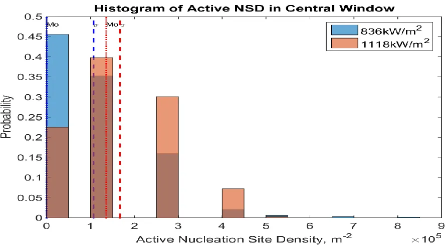
4.1.1 Active Nucleation Site Density (NSD)
Active NSD is the number of bubbles detected in each frame extrapolated to m-2 as shown in Figure 28.
Figure 29 Distribution of active NSD – lower heat fluxes, 621 samples each
Figure 31 Mean and mode of active NSD at all fluxes
Observation 4.1: Active NSD increases with heat flux as shown by the rightward shift of the
histograms. 1504kW/m2 is an exception to the trend.
Figure 32 Distribution of active NSD in Central Window (1.9 x 3.7mm2) - lower heat fluxes, 621 samples each
Figure 34 Mean & mode of active NSD in Central Window (1.9x3.7mm2) at all heat fluxes
Manual verification of the above observations has not been performed yet. It is probable that the reason for 1504kW/m2 exception and high central NSD at all fluxes is better bubble detection accuracy near the heater center.
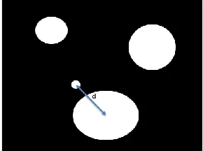
4.1.2 Minimum Nucleation Distance
Minimum nucleation distance is the center to center distance between a newly nucleated bubble and its nearest neighbor as shown in Figure 35.
Figure 36 Distribution of min. nucleation distance - lower heat fluxes, 203 & 292 samples respectively
Figure 37 Distribution of min. nucleation distance - higher heat fluxes, 319 & 488 samples respectively
Observation 4.2: Minimum nucleation distance reduces with heat flux. 1504 kW/m2 is an
Possible reasons for 1504 kW/m2 exception:
1. Several instances of only a single bubble being present over the entire heater area due to lesser residence time of bubbles
2. Slight increment in the total number of nucleation events over 1118kW/m2. 3. Less number of samples to correctly identify the trend
4.1.3 Nucleation Rate
Nucleation rate is the number of new bubbles nucleated per millisecond (m-2ms-1) on the heater’s surface. Since 62ms of data is analyzed, the sample space consists of 62 data points.
Figure 39 Distribution of bubble nucleation rate - higher heat fluxes
Observation 4.3: Nucleation rate increases with heat flux. A large jump is observed at CHF
as is indicated by the large rightward shift of the 1893kW/m2 histogram.
Observation 4.4: 1504 kW/m2 is not an exception here.
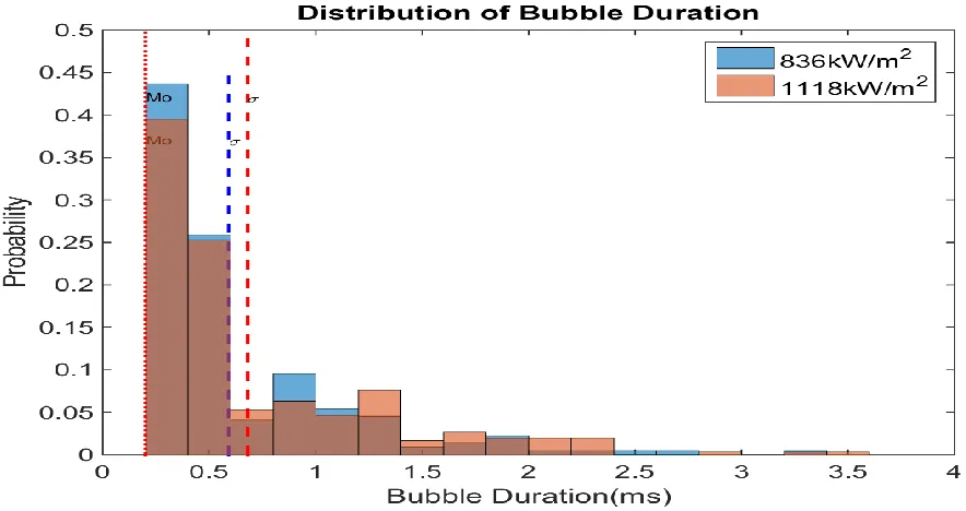
4.1.4 Residence Time (tres)
Residence time is the time between when the bubble was first detected and the last time of its detection as shown in Figure 40.
Figure 40 Progression of bubble area in sequential frame used to determine bubble residence time
Figure 42 Distribution of bubble residence time - higher heat fluxes, 326 & 490 samples respectively
Observation 4.5: Within the limits of uncertainty in data, mean residence time of bubbles
remains same with increasing heat flux.
As noted in Observation 4.4, bubbles seem to last longer at 1118kW/m2 than at any other heat flux. The reason is not know yet.
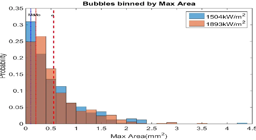
4.1.5 Maximum Bubble Area
Maximum bubble area is the maximum area reached by the bubble during its evolution.
Figure 43 Distribution of max bubble area - lower heat fluxes, 220 & 301 samples respectively
Observation 4.6: Maximum bubble area increases slightly with heat flux as seen in the
rightward shift of the histograms.
Note that the bubble departure diameter in pool boiling decreases with heat flux.
4.1.6 Area Expansion Velocity
Area expansion velocity (EV) is defined as the ratio of maximum bubble area to the time taken to reach it (tmax area). In most cases, bubbles are tracked until they reach their maximum area (tmax area = tres), due to the chaotic nature of collapse being hard to capture autonomously. In some instances, the collapse process of the bubble is identified and here tmax area < tres.
Figure 46 Distribution of bubble area expansion velocity - higher heat fluxes, 326 & 490 samples respectively
Observation 4.7: The area expansion velocity increases with heat flux.
The increase in expansion velocity with heat flux can be explained by assuming quasi-equilibrium evaporation (injected liquid temperature = Tsat) process at the heater surface as shown in Figure 47.
𝑗 = 𝑞 ′′
𝐻𝐿𝑉
Where j is the vapor mass flux, q’’ is the heat flux and HLV is the latent heat of vaporization. Since more vapor mass flux needs to be created at higher heat fluxes, the bubble base area expands faster. In reality, the evaporation process is non equilibrium but the vapor mass flux is still directly proportional to heat flux.
It appears that with increasing heat fluxes bubbles reside longer after attaining maximum bubble area since average tres and average maximum bubble area do not change significantly. The area expansion velocity is averaged over the bubble’s expansion time. It does not reflect the instantaneous motion of its boundary which is shown below.
4.1.7 Average Instantaneous Expansion Velocity
Consider 2 bubbles nucleated anywhere on the heater not necessarily simultaneously. The first bubble expands for 0.5ms and the second expands for 0.8ms. For each bubble: Instantaneous EVs at 0.3ms, EV1 and EV2 = (Area at 0.4ms – Area at 0.3ms) / 0.1ms and average instantaneous EV at 0.3ms = (EV1 + EV2) / 2
Figure 48 Increasing average instantaneous expansion velocity at different heat fluxes
Observation 4.8: In general, the bubble bases expand in an accelerating manner with time
Here, only those bubbles are considered which have an area less than 0.06mm2 (diameter = 0.27mm) at the time of initial detection. This is a new finding and has not been found in literature.
Based on accelerating expansion of bubbles, a probable explanation is that the region
surrounding the nucleation sites is hotter than the site. The BETA experiments confirmed that regions surrounding nucleation sites is hotter than the sites using high resolution IR imaging techniques. (Liu & Dinh, 2015)
4.2 Secondary Analysis
nucleated from sites constituting the cluster or in-pattern bubbles are compared with out-of-pattern bubbles’ characteristics in the search for critical behavior near CHF.
4.2.1 Identification of High Frequency Nucleation Site Cluster
Analysis of spatial distribution of bubbles or accumulative NSD reveals local regions of high nucleation activity on the heater surface as shown in Figure 49. The centers of bubbles at initial detection are denoted by a red dot that marks a nucleation site. Several dots were observed in ‘close proximity’ to each other, marking a nucleation site with high nucleation activity. It was experimentally found that dividing the entire heater surface into square elements 7x7 pixels in size, encapsulated the maximum number of proximal red dots at each heat flux while keeping the element area (0.028mm2) to a minimum. Therefore, a nucleation site is denoted by a square element for convenience.
As an aside, the proximal red dots do not overlap because of the following:
1. Pinching: According to the current understanding of nucleation, once a bubble departs (pool boiling) or collapses (film boiling), remnants of vapor are ‘pinched off’ at the heater surface. The pinching could occur stochastically at any nucleation site present under the expanded bubble. That remnant vapor reduces the nucleation energy barrier at the site and makes subsequent nucleation easier. The probability of pinching is high at regions that have been exposed to vapor for a longer time i.e. regions close to the nucleation site.
4.2.1.1 Accumulative Nucleation Site Density (NSD)
Accumulative NSD signifies the total number of nucleation events over the entire heater surface in the time duration under consideration (62ms). Nucleation sites are classified based on nucleation frequency:
Regular Nucleation Site (RNS): A 7x7 pixel square element containing more than one red dot which implies that the site had multiple nucleation events within 62ms.All RNS are part
of high nucleation frequency cluster constituting the nucleation pattern. Bubbles nucleated at
these sites are called regular bubbles.
Figure 49 Variation in distribution of accumulative NSD with heat flux
The color of the square element shows the number of red dots contained within it or the nucleation site’s frequency. It can be read by using the color bar.
The legend indicates the total number of bubble observations (samples or red dots) and accumulative NSD (m-2) based on total number of bubbles detected in 62ms.
Figure 50 Nucleation statistics
Observation 4.9: a) Surface averaged nucleation frequency i.e. ratio of number of regular
bubbles (Gray line) to the number of RNS (Orange line) increases with heat flux. No fixed
trend can be observed for the bubbles nucleated at INS.
b) Preliminary analysis of RNS present at all fluxes, shows that for a fixed site, the
nucleation frequency either increases or stays the same with increasing flux.
c) The site with the maximum nucleation events changes with heat flux.
Observation 4.10: In the central region and at all fluxes, large areas where nucleation does
not take place at all are present near regions of high nucleation activity.
Upon further investigation it was found that during the observation period of 62ms, regions with no nucleation were covered with vapor from neighboring bubbles as shown in Figure 51 for 1504kW/m2. In the bubble footprint (L), the color white represents the accumulative
0 50 100 150 200 250 300 350
800 1000 1200 1400 1600 1800 2000
N
u
m
b
er
Heat Flux kW/m^2
Site Behavior
# of sites (rectangle = red dots) that nucleate once
# of sites(rectangles) that nucleate more than once
vapor fraction within the 62ms period i.e. whiter regions have been covered with vapor more frequently.
Figure 51 Vapor coverage (L) through nucleation (R) in neighborhood at 1504kW/m2
Observation 4.11: Frequent vapor coverage from neighboring bubbles inhibits nucleation
Observation 4.11 suggests that regular bubbles inhibit the occurrence of irregular bubbles in their neighborhood. It appears that nucleation in INS occurs when the spatiotemporal
nucleation pattern is disrupted. Such disruptions could occur due to slight spatial variations in the location of cluster sites caused due to ‘pinching’ or temporal pattern variations due to delay in nucleation of the order of 0.1ms. These disruptions force the heater-microlayer system to nucleate out-of-pattern irregular bubbles at INS.
4.2.2 Spatial Analysis of Pattern
critical behavior near CHF. Site averaged idle time (tidle), a RNS characteristic, is also analyzed.
*In the following visualizations, the word ‘mean’ is used to denote surface averaged values.
4.2.2.1 Maximum Diameter (DMax)
The color bar indicates the site averaged maximum diameter.
4.2.2.1.1 Spatial distribution of bubble DMAX at INS (DMAX,Irr)
4.2.2.1.2 Spatial distribution of site averaged bubble DMAX at RNS (DMAX,Reg)
Figure 53 Variation in distribution of site averaged bubble DMAX at regular sites with heat flux
As expected, both mean DMAX,Reg and mean DMAX,Irr increase with flux.
Observation 4.12: In preliminary analysis of regular sites present at all heat fluxes, the site
averaged DMAX,Reg first increased and then decreased with increasing flux. No consistent
relation could be found between site averaged DMAX and site nucleation frequency.
Observation 4.13: At all fluxes, irregular bubbles are generally smaller than regular
Considering the uncertainty in image processing and the small difference in the mean values, not much significance is attributed to this observation. However, this type of information gives credibility to the disruptive nature of irregular bubbles by confirming that in-pattern regular bubbles are larger and therefore better at removing heat.
4.2.2.2 Residence Time (tres)
The color bar indicates the site averaged residence time.
4.2.2.2.1 Spatial distribution of bubble tres at INS (tres,Irr)
4.2.2.2.2 Spatial distribution of site averaged bubble tres at RNS (tres,Reg)
Figure 55 Variation in the distribution of site averaged bubble tres at regular sites with heat flux
Mean tres,Reg reduced by 0.1ms at high heat fluxes and mean tres,Irr does not change appreciably with heat flux.
At 836kW/m2 the high value of mean tres,reg is due to an image processing aberration.
Observation 4.14: At all heat fluxes, irregular bubbles have lesser residence time compared
Again, given the uncertainty, this small difference is ignored. However, this suggests that irregular bubbles are incidental and the incident likely leads to a local temperature spike responsible for their nucleation.
Observation 4.15: Sites that have large site averaged bubble residence times are spatially
isolated at each heat flux.
4.2.2.3 Idle Time (tidle)
The color bar indicates the site averaged idle time.
Observation 4.16: Mean tidle reduces linearly with increasing heat flux and site averaged tidle
reduces as site frequency increases. 𝐹𝑟𝑒𝑞𝑢𝑒𝑛𝑐𝑦 = 1
𝑡𝑖𝑑𝑙𝑒+𝑡𝑟𝑒𝑠
Further investigation revealed that the majority of the idle times are close to the site averaged tidle while others show wide variation. Site averaging of bubble characteristics assumes temporal and thermal uniformity at the site which is an outcome of a stable spatio temporal pattern. Wide variations in idle times makes this process questionable since it indicates different thermal conditions at the time of nucleation. Possible explanation for these variations include:
4.2.2.4 Area Expansion Velocity
The color bar indicates the site averaged expansion velocity.
4.2.2.4.1 Spatial distribution of Area Expansion Velocity at INS (EVIrr)
4.2.2.4.2 Spatial distribution of Area Expansion Velocity at RNS (EVReg)
Figure 58 Variation in the distribution of site averaged area expansion velocity at regular sites with heat flux
Expansion velocity increases with heat flux.
Observation 4.17: Preliminary analysis of regular sites present at all fluxes shows that, site
averaged EV follows the trend of site averaged DMAX.
Observation 4.18: Mean EVReg > mean EVIrr at all heat fluxes. There is a large difference at
higher heat fluxes.
However, sites with maximum nucleation frequency at each heat flux do not have the highest site averaged expansion velocity.
Since irregular bubbles nucleate in hotter regions, greater expansion velocity of regular bubbles is unexpected. The reason is not known yet.
4.3 Errors, Biases and Uncertainty in Data Analysis
The following biases occur in BETA-B data analysis. The first three are features that increase data robustness by adding a small bias. Points 4 and 5 detail inadvertent errors. Points 6 and 7 highlight major biases by critiquing the averaging involved in the methods used.
1. The initial size of a bubble at the time of detection will be greater than 0.02mm2 (25 pixels). All objects less than 25 pixels are removed from picture as part of noise removal. This results in “stubborn” bubbles not being identified. It also impacts bubble
characteristics like residence time and initial expansion velocity.
2. Only bubbles that exist and are expanding for a duration longer than 0.2ms after initial detection are considered in all analysis. This enhances data robustness by removing ‘False Positives’ but also introduces bias in the form of removing bubbles with residence time < 0.2ms. This impacts bubble nucleation characteristics e.g. Active NSD,
accumulative NSD, minimum nucleation distance and nucleation rate.
4. Another error source is ‘re-detection’ of the same bubble due to a segmentation error in image processing resulting in a bubble being divided into:
a. Two non-bubbles: This results in the identification and tracking of two separate bubbles before and after incorrect segmentation. It increases nucleation frequency at RNS and affects all site averaged properties, particularly, idle time.
b. Two bubbles: One bubble is tracked as if the incorrect segmentation did not happen. It will result in a loss of area at the instance of incorrect segmentation. The other bubble is tracked as a new nucleation center from the moment of segmentation. This increases the number of INS in the neighborhood of RNS. c. One bubble and one non-bubble: This is the best case and results in just loss of
area at the moment of segmentation.
5. The area element dimension choice (7x7 pixels) and its fixed spatial location introduces uncertainty in post-processing, occurring when proximal red dots are located across multiple elements, resulting in
a. Reduction of observed nucleation frequency at the erroneous regular site b. Increase in irregular bubbles or incorrectly grouped regular bubbles. 6. Statistical analysis of nucleation characteristics involves spatial averaging of data.
4.4 Summary
Data analysis of BETA-B data at 4 different heat fluxes 836 kW/m2, 1118 kW/m2,
1504kW/m2 and 1893 kW/m2 provides key insights into high heat flux nucleate boiling. The results of primary statistical are shown in Table 1.
Table 1 Observations from primary analysis
1. Active NSD increases with heat flux. 1.5-2 times more bubbles are nucleated near the heater center than near the heater periphery. The reason is not known.
2. Nucleation rate increases with heat flux. A large jump is observed at CHF.
3. Minimum nucleation distance reduces with heat flux
4. Mean residence time of bubbles remains same. This is different from significant reduction in residence time in pool boiling, reported in literature.
5. Maximum bubble area increases slightly with heat flux. This opposes the trend reported in literature for departure diameter in pool boiling.
6. The area expansion velocity increases with heat flux