Impact of Human Affectiveness Metrics and Attribute Selection on software productivity.

(1)

ABSTRACT

RAVICHANDRAN, SUSHMA. Impact of Human Affectiveness Metrics and Attribute Selection on software productivity. (Under the direction of Dr. Timothy Menzies.)

In a collaborative software development environment, the sentiments, politeness and/or emotions (collectively called ‘affectiveness‘) of a developer is said to have direct implica-tions on the time taken to complete the development task. To be able to computationally identify and categorize opinions expressed in a piece of text, in order to determine whether the writer’s attitude towards a particular topic is positive, negative, or neutral is an ad-vantage of today’s technologically progressive world. There have been many studies that compare the sentiments shared by the developer who reports a GitHub Issue, with the issue resolution time (i.e software productivity) which show that issues representing LOVE and JOY decrease issue resolution time whereas issues representing SADNESS increase issue resolution time. These researchers have concluded that a positive sentiment drives software productivity whereas a negative sentiment slows it down.

(2)

(3)

Impact of Human Affectiveness Metrics and Attribute Selection on software productivity

by

Sushma Ravichandran

A thesis submitted to the Graduate Faculty of North Carolina State University

in partial fulfillment of the requirements for the Degree of

Master of Science

Computer Science

Raleigh, North Carolina 2017

APPROVED BY:

Dr. Christopher Parnin Dr. Min Chi

(4)

DEDICATION

(5)

BIOGRAPHY

(6)

ACKNOWLEDGEMENTS

I am most privileged to have worked with my advisor Dr. Timothy Menzies. I thank him for not only sharing his wealth of knowledge and always pushing me to strive towards excellence but also for being a huge source of guidance to complete this work successfully.

I am grateful to Dr. Christopher Parnin and Dr. Min Chi, members of my Advisory Committee for sharing their valuable inputs to bring the thesis to its current shape.

(7)

LIST OF TABLES

Table 3.1 Dataset Details . . . 14

Table 3.2 Extracted Control Metrics Features . . . 15

Table 3.3 Extracted Affective Metrics Features . . . 16

Table 3.4 Examples of Sentiment tool . . . 17

Table 3.5 Examples of Emotions tool . . . 19

Table 3.6 Affective Metrics Details . . . 20

Table 4.1 Features removed after Attribute Selection Pt 1 . . . 27

Table 4.2 Features removed after Attribute Selection Pt 2 . . . 28

Table 5.1 Confusion Matrix . . . 31

Table 5.2 Classification of scikit Data set . . . 33

Table 5.3 Classification of vue Data set . . . 34

Table 5.4 Classification of titan Data set . . . 35

Table 5.5 Classification of tensor Data set . . . 36

Table 5.6 Classification of swift Data set . . . 37

Table 5.7 Classification of storm Data set . . . 38

Table 6.1 Summary Table: Performance Metrics . . . 55

(9)

LIST OF FIGURES

Figure 4.1 A Comparison of Filters and Wrappers . . . 24 Figure 6.1 Sample Scott Knott Results that prefer Control over Affective Metrics 43 Figure 6.2 Sample Scott Knott Results that prefer Affective over Control Metrics 44 Figure 6.3 Scikit and Storm False Alarm Statistics. The results in red do not

endorse the thesis of this report . . . 46 Figure 6.4 Swift and Tensor False Alarm Statistics. The results in red do not

endorse the thesis of this report . . . 47 Figure 6.5 Titan and Vue False Alarm Statistics. The results in red do not endorse

the thesis of this report . . . 48 Figure 6.6 Scikit and Storm Recall Statistics. The results in red do not endorse

the thesis of this report . . . 49 Figure 6.7 Swift and Tensor Recall Statistics. The results in red do not endorse

the thesis of this report . . . 50 Figure 6.8 Titan and Vue Recall Statistics. The results in red do not endorse the

thesis of this report . . . 51 Figure 6.9 Scikit and Storm Precision Statistics. The results in red do not endorse

the thesis of this report . . . 52 Figure 6.10 Swift and Tensor Precision Statistics. The results in red do not endorse

the thesis of this report . . . 53 Figure 6.11 Titan and Vue Precision Statistics. The results in red do not endorse

(10)

CHAPTER

1 INTRODUCTION

In reference to the sentiments shared in Issue reports,[1]said:

Emotions such as JOY and LOVE reduce the resolution time, whereas emo-tions such as SADNESS increase the issue resolution time.

(11)

1.1 Background

Software Development Projects especially in a distributed team in multiple locations in-volve a number of developers, each having a different mannerism, background, working environment and working hours. Employees generally communicate via distributed version control and source code management systems such as Git. Git is a repository hosting service which makes contributing to and documenting Open Source projects straightforward and convenient.

Git Issues are an elegant way to keep track of tasks, enhancements, and bugs for such projects. An issue can be raised by one member of a team to point out the probable areas of concern for a piece of code. The other members of the team, including the person(s) responsible for the code can discuss the raised issue, resolve it by taking the necessary actions and then close the issue. This time period from the time of issue creation to the time at which the issue was closed is called the issue resolution time. It is a highly variable number and is closely related to the developer productivity.

Productivity of a software is measured in Open Source projects such as the ones in Git by the duration of its issues. To be able to thus, predict the productivity of a software development or the length of its issues is an attractive area of research.

(12)

generally include the contents of comments, issue title and issue body.

Humans invariably perceive and/or present some form of sentiment and these senti-ments are exhibited consciously or unconsciously while sending out issue reports to fellow employees.

The implications of emotions on the productivity of other developers working on the same project is an interesting one. Authors of[1]proved that positive sentiments aids the productivity of a project and issues containing anger or sadness took a longer time to resolve. They also proved that better results in predicting the resolution time of an issue was obtained when the emotions of a developer were taken into picture. This shows that emotions are an important criteria in the work rate of a development project.

Although[1]has been able to practically describe the general notion that happiness increases productivity and sadness decreases productivity, the increase in recall and pre-cision is very minimal after appending the affective factors. Also, there needs to be an understanding on whether the addition of affective factors is mandatory for predicting is-sue resolution time. This thesis attempts to reproduce the work done in[1]and experiments with dimensionality reduction to produce comparably precise results.

1.2 General Motivation

(13)

anger and sadness. These are collectively called human ‘affectiveness‘ factors. This thesis revolves around this interesting factor. It aims to learn how important such cognitive factors are for the development of a software product. For this purpose, the sentiments shared in code sharing portals like github where developers interact with each other purely via textual contents was taken advantage of. The sentiments from issues was extracted and compared to how quickly different issues were resolved thereby producing a model that compares sentiments with productivity.

Another factor to note here is the constant difficulty software engineering researchers face while performing sentiment analysis tasks on software engineering datasets. Most of the machine learning tools commonly used for content analysis are trained with literature novels and newspaper/magazine articles. This kind of text is different from those shared in software engineering datasets. Not having been trained by the correct training set, may affect the accuracy of predicting the sentiments/affectiveness. Hence, a learning model that is trained for guaranteed precise prediction with software engineering data is an ulterior motive behind such research ventures.

1.3 Statement of The Thesis

(14)

1.4 Publication from this Thesis

There are no publications from this thesis.

1.5 Structure of the Thesis

(15)

CHAPTER

2 RELATED WORK

(16)

used. Hence, although information retrieval is an important aspect on any content shar-ing environment, generic opinion minshar-ing learnshar-ing models cannot be used for software engineering data.

The study of affect in a workplace gained a lot of momentum in the 1990s. A lot of critical thinking went into determining the concept of job satisfaction which was a loosely defined term until then. Brief et al in[5]for example conduct a survey on the effects of moods and emotions experienced in workplace. Their research addresses the various theoretical and methodological opportunities and challenges involved in gauging affect in the workplace. The affective status of the job satisfaction construct is assessed very briefly followed by a survey of the effects of moods and emotions experienced in the workplace. Conceptual concerns about workers‘ feelings not adequately addressed in the organizational literature were raised, and suggestions for how to approach these concerns methodologically were provided. Overall, the intent of the paper was to appraise what is known about affective experiences in organizational settings, to highlight existing gaps in the literature, and to suggest how those gaps might be filled. They also highlight the importance of a two way influence- workplace on people and people on workplace.

Erez et al in[6]conducted two studies which indicated that positive affect along with work environment influences motivation and that its influence on motivation occurs not through general effects, such as response bias or general activation, but rather through its influence on the cognitive processes involved in motivation.

(17)

attitudes in software engineering processes and tools and present initial results from an empirical study investigating correlations between personality and attitudes to software engineering processes and tools. They discuss what are currently hindering a more wide-spread use of psychometrics and how overcoming these hurdles could lead to a more individualized software engineering. They conclude that Software Engineering researchers should put a larger focus on the humans involved in software development than what has been done to date. One easy and powerful way to do this would be to collect psychometric measurements.

On similar lines, authors of[8]discuss the relevance of emotions in determining work results and how team members collaborate in a project. They drew emotion summaries from software development projects and concluded that their results were in good correla-tion with the emocorrela-tion state of the project after interviewing project leaders. However, the interviews also indicate that the current state of the summaries is not detailed enough and further improvements are needed.

(18)

forming work teams, project managers and lecturers should carry out a personality test beforehand in order to balance the amount of extraverted team members with those who are not extraverted. This would permit the team members to feel satisfied with the work carried out by the team without reducing the quality of the software products developed. As an alternative, Sinha et al in[9]performed sentiment analysis on commit logs. The commits were first divided into small, medium and large commits. They aimed to find correlations between the sentiments expressed in commit logs and the number of files changed. Although a majority of the sentiment was neutral, the negative sentiment was about 10% more than the positive sentiment overall. Tuesdays seemed to have the most negative sentiment overall. In addition, they find a strong correlation between the number of files changed and the sentiment expressed by the commits the files were part of. Future work and implications of these results were also discussed.

In[12]the authors used their framework to study the relationship between politeness and social power, showing that polite Wikipedia editors are more likely to achieve high status through elections, but, once elevated, they become less polite. Similar negative correlation between politeness and power were seen on Stack Exchange, where users at the top of the reputation scale were less polite than those at the bottom. Finally, classifier was applied to a preliminary analysis of politeness variation by gender and community.

In a slightly different research venture, to increase the positivity in a work environment, [31]introduced the idea of gamification in workplace. They present Gamiware, a gamifica-tion platform aimed to increase motivagamifica-tion in software projects which is rounded on both gamification roots and in software process improvement initiatives.

(19)

productivity of a software development team. For example[29]argues that a synthesized view of the emerging human-focused SE research is needed and can add value through giving focus, direction and help identify gaps. Taking cues from the addition of Behavioral Economics as an important part of the area of Economics, the paper proposes the term Behavioral Software Engineering (BSE) as an umbrella concept for research that focus on behavioral and social aspects in the work activities of software engineers.

In[30], the authors claim that affective states - emotions, moods, and feelings - have an impact on work-related behaviors, cognitive processing activities, and the productivity of individuals. They report an empirical study on the impact of affective states on software developers performance while programming. They also demonstrate the value of applying psychometrics in Software Engineering studies.

Acuna et al[32]present aggregate results of an experiment that evaluates the relation-ships between personality, team climate, product quality and satisfaction in software de-velopment teams. Their experimental study measures the personalities of team mem-bers based on the Big Five personality traits (openness, conscientiousness, extraversion, agreeableness, neuroticism) and team climate factors (participative safety, support for innovation, team vision and task orientation) preferences and perceptions.

(20)

Ortu et al[4]performed analysis on the issue comments of 14 projects under the JIRA repository. They studied the politeness of these comments to see if it has any relation with the number of developers involved in these projects over time. They also checked if it has any relation with the time required to fix any issue. Results from both these tests showed that the sentiments of issue comments did affect them. In comparison with all this work done previously, the authors of[1]considered three kinds of affective metrics - politeness, emotions and sentiments and compared the influence of all these factors on the issue resolution time. They found that issues that expressed positive emotions took lesser time to resolve as compared to those that expressed negative emotions. They use logistic regression to deduce the same.

(21)

CHAPTER

3 METHOD

(22)

body, title and comments).

These were then passed through three classifiers-j48, Naive Bayes and Random Forest. The results obtained were noted down. Next, feature Selection was performed on the four metrics using a method called Wrapper Subset Eval. Only those features which contributed (higher than a threshold value) to predicting the class of the issue duration (short/long) was chosen. These feature subset of metrics were passed through the same classifiers and the results obtained were compared to the previous set of results of complete models with all features included.

The precision, recall and false alarm obtained in all cases were noted down and a Scott-Knott Analysis was performed to further examine the results.

3.1 Data

The dataset comprised of GitHub records of Open Source Projects. Git is an open source version control system similar to subversion, mercurial and CVS. Version control is a system that records changes to a file or set of files over time so that you can recall specific versions later. It allows you to revert files back to a previous state, revert the entire project back to a previous state, compare changes over time, see who last modified something that might be causing a problem, who introduced an issue and when, and more.

(23)

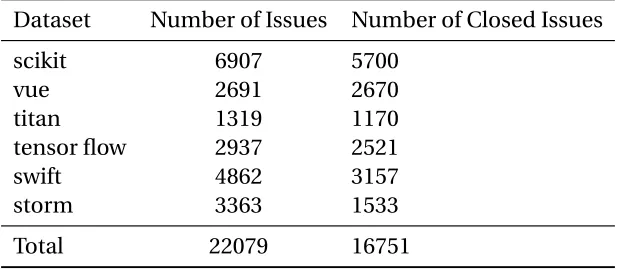
Table 3.1Dataset Details

Dataset Number of Issues Number of Closed Issues

scikit 6907 5700

titan 1319 1170

tensor flow 2937 2521

swift 4862 3157

storm 3363 1533

Total 22079 16751

with them. This is important in the research as the software productivity is closely aligned with the duration of an issue.

Table 3.1 shows the details of the contents of each of these datasets. As shown, a total of about 17,000 files were studied and their content analysed. Python scripts were written to extract the necessary features.

3.2 Control Metrics

(24)

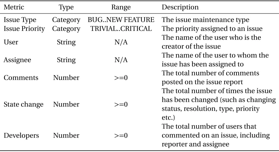
Table 3.2Extracted Control Metrics Features

Metric Type Range Description

Issue Type Category BUG..NEW FEATURE The issue maintenance type Issue Priority Category TRIVIAL..CRITICAL The priority assigned to an issue

User String N/A The name of the user who is the

creator of the issue

Assignee String N/A The name of the user to whom the

issue has been assigned to

Comments Number >=0 The total number of comments

posted on the issue report

State change Number >=0

The total number of times the issue has been changed (such as changing status, resolution, type, priority etc.)

Developers Number >=0

(25)

Table 3.3Extracted Affective Metrics Features

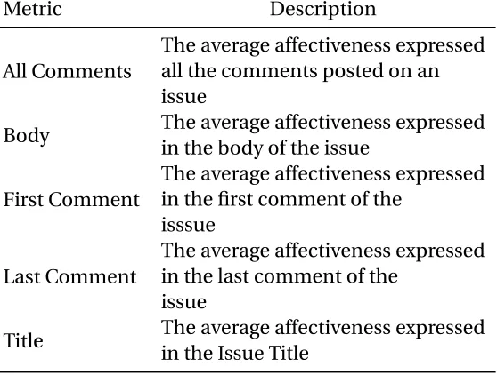
Metric Description

All Comments

The average affectiveness expressed all the comments posted on an issue

Body The average affectiveness expressed in the body of the issue

First Comment

The average affectiveness expressed in the first comment of the

isssue

Last Comment

The average affectiveness expressed in the last comment of the

issue

Title The average affectiveness expressed in the Issue Title

the Table 3.2

3.3 Affective Metrics Features

(26)

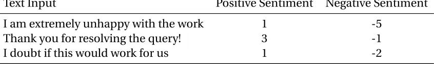
Table 3.4Examples of Sentiment tool

Text Input Positive Sentiment Negative Sentiment

I am extremely unhappy with the work 1 -5

Thank you for resolving the query! 3 -1

I doubt if this would work for us 1 -2

3.3.1 Sentiments

Sentiments were analysed using a tool called SentiStrength[11]which estimates the degree of positive or negative sentiments in English sentences. SentiStrength estimates the strength of positive and negative sentiment in short texts, even for informal language. It was originally developed for English and optimised for general short social web texts. It assigns an integral value (in the range -5 to+5) to every sentence. A positive sentiment indicates that the sentence is positively polarised where 1 is slightly positive and 5 is extremely positive. A negative sentiment indicates that the sentence is negatively polarised where -1 indicates slightly negative and -5 indicates extremely negative.

(27)

3.3.2 Politeness

To extract the degree of politeness from texts, we use a technique devised by Daniscu et al.[12]. The machine learning approach was originally designed to evaluate the politenesss in Wikipedia and StackOverflow posts. Their framework was used to study the relationship between politeness and social power, showing that polite Wikipedia editors are more likely to achieve high status through elections, but, once elevated, they become less polite. Similar negative correlation was seen between politeness and power on Stack Exchange, where users at the top of the reputation scale were less polite than those at the bottom.

Stack OverFlow is a Q and A Forum with many software and computer science related questions. As the tool was designed for data of similar format, it could be applied to the domain considered in this thesis. The tool classifies each sentence as ‘polite‘ or ‘impolite‘. Apart from this label, the tool also specifies a level of confidence related to the probability of the politeness class being assigned. In the current work, we considered the cases only when the confidence label was above 0.5. In other cases we marked the issues as ‘neutral‘.

As with sentiment extraction, this tool is also available for free academic research and was previously used by the authors of[1]in their work.

3.3.3 Emotions

Emotions extracted from issues are the third affective metrics this thesis takes into consid-eration. Similar to Murgia et al.[13]and Ortu et al[1]Parrot’s emotional frameworks were used. It consists of six emotions- joy, sadness, love, anger, surprise, and fear.

(28)

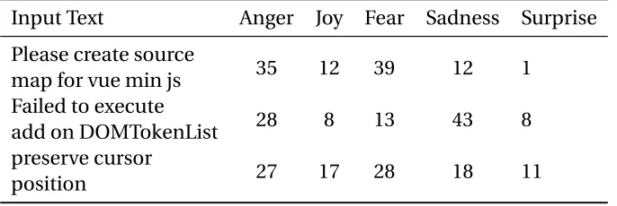
Table 3.5Examples of Emotions tool

Input Text Anger Joy Fear Sadness Surprise

Please create source

map for vue min js 35 12 39 12 1

Failed to execute

add on DOMTokenList 28 8 13 43 8

preserve cursor

position 27 17 28 18 11

analysis tool such as the ones available for measuring sentiment and politeness. For this reason, they had built a machine learning classifier that was able to identify the presence of four basic emotions: JOY, LOVE, ANGER and SADNESS (these are the most popular emotions identified by Murgia et al.[13]in issue comments). There has been a considerable amount of work in this area ever since. Works in[18][19][20][21]all built different kinds of emotion taggers on text data, but an easy to use model for research purposes was still unavailable then.

At this point however, a tool[14]that does the necessary text analytics to classify text based on the emotions it conveys was found. It has a number of APIs for different kinds of analytics purposes. We are interested in the Emotion API that classifies text into five different kinds of emotions - Anger, Joy, Fear, Sadness and Surprise.

The API requires a text input and it generates a percentage presence of each of the emotions in the text.

(29)

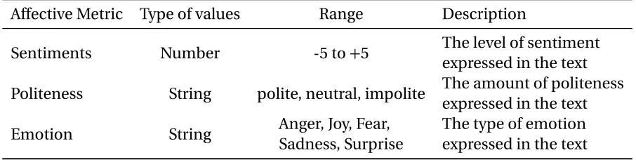
Table 3.6Affective Metrics Details

Affective Metric Type of values Range Description

Sentiments Number -5 to+5 The level of sentiment

expressed in the text Politeness String polite, neutral, impolite The amount of politeness

expressed in the text

Emotion String Anger, Joy, Fear,

Sadness, Surprise

The type of emotion expressed in the text

metrics- politeness, sentiments and emotions. Each of these was run through a classifier and the results were recorded. Next, feature selection was performed on each of the four data metrics of each dataset.

3.3.4 Dependent Variable

(30)

CHAPTER

4 FEATURE SELECTION

(31)

In machine learning and statistics, feature selection, also known as variable selection, attribute selection or variable subset selection, is the process of selecting a subset of relevant features (variables, predictors) for use in model construction.

The basis of this idea is that data consists of features that may be redundant or irrelevant. By performing feature selection these features can be removed without any or little loss of information. Feature Selection is performed on each of the four data metrics of each dataset.

There are many methods used for the process of Feature Selection in Data Science. One such is the Information Gain Technique. In decision tree learning, Information gain ratio is a ratio of information gain to the intrinsic information. It is used to reduce a bias towards multi-valued attributes by taking the number and size of branches into account when choosing an attribute. Information Gain is also known as Mutual Information. The problem with Information Gain is that it only ranks single attributes.

Correlation based Feature Selection[22]or CFS does better than Information Gain because it ranks sets of attributes. It evaluates subsets of features on the basis of the following hypothesis: ‘Good feature subsets contain features highly correlated with the classification, yet uncorrelated to each other‘.

Unlike some other feature selectors (e.g. Relief, InfoGain), CFS evalautes and hence ranks feature subsets rather than individual features. CFS performs a best-first search (with a horizon of five1) to discover interesting sets of features

Hall et al. scores each feature subsets as follows:

1_{(1) The initial “frontier” is all sets containing one different feature. (2) The frontier of size}_n_(initially_n₌₁₎

(32)

merits =

k rcf

Æ

k+k(k−1)rff

where:

merits is the value of some subsetsof the features containingk features;

rcf is a score describing the connection of that feature set to the class;

andrff is the mean score of the feature to feature connection between the items ins.

Note that for this to be maximal,rcf must be large andrff must be small. That is, features

have to connect more to the class than each other.

The above equation is actually Pearson’s correlation where all variables have been standardized. To be applied for discrete class learning (as done by KDP and this paper), Hall et al. employ the Fayyad Irani discretizer[23]then apply the following entropy-based measure to inferr (the degree of associations between discrete setsX andY):

r_xy=2_×H(x)+_H₍H_y(₎₊y)_H−₍H_x(₎x,y)

(33)

Figure 4.1A Comparison of Filters and Wrappers

from your own Java code. Weka contains tools for data pre-processing, classification, regres-sion, clustering, association rules, and visualization. It is also well-suited for developing new machine learning schemes. It is open source software issued under the GNU General Public License.

(34)

small changes in the training data distribution. Using the full training set for attribute selection means that the algorithm is just run once on all the data.

Weka‘s WrapperSubsetEval implements the method described by Kohavi in his papers on wrapper feature selection. That is, it performs repeated 5-fold cross-validation internally on the training data in order to evaluate the ‘merit‘ of a given subset of features. Note that this cross-validation process is completely separate from the outer cross-validation performed by the attribute selection CV mode described above.

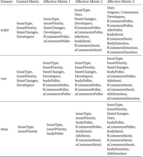
Control Metric as the name suggests includes all the control features such as issue type, issue priority, user, Assignee, Comments, stateChanges and Developers. Affective Metric 1 includes the control metrics and the features obtained after extracting the degree of politeness from issue title, issue body, first comment in each issue, last comment in each issue and average politeness from all comments of each issue. These have been labelled issueTitle, issueBody, fCommentPolite, lCommentPolite and aCommentPolite. Similarly Affective Metric 2 and 3 are features obtained from the Sentiment and Emotion model as explained previously.

Table 4.1 and 4.2 show a list of features that were removed using the WrapperSubsetEval process. Each row in the two tables represent each of the six datasets. The columns indi-cate each of the four data metrics. The values show the list of features that were deemed unimportant for the machine learning classifier.

(35)

of an issue and issue body. From the control metrics, features such as user, comments and assignee were regarded important. From the affective metrics, politeness from issue body, emotion from issue body and from all of the issue’s comments and average of the sentiments from issue comments were regarded important.

(36)

Table 4.1Features removed after Attribute Selection Pt 1

Dataset Control Metric Affective Metric 1 Affective Metric 2 Affective Metric 3

(37)

Table 4.2Features removed after Attribute Selection Pt 2

Dataset Control Metric Affective Metric 1 Affective Metric 2 Affective Metric 3

(38)

CHAPTER

5 RESULTS

This chapter presents the numeric results for when different attribute sets were used to predict for issue close time. Chapter 6 performs a statistical analysis on this data.

At this point for each of the six datasets, eight different data metrics were generated-four before feature selection and generated-four more after. A control metric, three different affective metrics (for politeness, sentiment and for emotions) and four metrics after performing WrapperSubsetEval[16]on each of these data metrics.

(39)

Forest. Naive Bayes is a simple technique for constructing classifiers: models that assign class labels to problem instances, represented as vectors of feature values, where the class labels are drawn from some finite set. Naive bayes is a classification technique based on Bayes’ Theorem with an assumption of independence among predictors. In simple terms, a Naive Bayes classifier assumes that the presence of a particular feature in a class is unrelated to the presence of any other feature. Naive Bayes classifiers are highly scalable, requiring a number of parameters linear in the number of variables (features/predictors) in a learning problem.

(40)

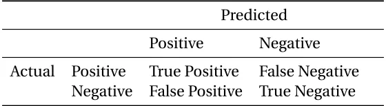
Table 5.1Confusion Matrix

Predicted Positive Negative Actual Positive True Positive False Negative

Negative False Positive True Negative

machine learning method for classification and regression. They construct a number of decision trees during training and for each data object they output the class that is the mode of the classes (classification) or mean prediction (regression) of the individual decision trees. Random forests correct for decision trees’ habit of overfitting their training set.

In our work, we ran all 8 datasets in each of the three learners and observed the results. Specifically, the results from its confusion matrix were noted and precision, recall and false positive values were calculated. A confusion matrix is a table that is often used to describe the performance of a classification model (or "classifier") on a set of test data for which the true values are known. Table 5.1 shows a confusion matrix. The formulae for calculating Precision, Recall and False Alarm are as follows:

Precision= True Positive

True Positive+False Positive (5.1)

Recall= True Positive

True Positive+False Negative (5.2)

False Alarm= False Positive

False Positive+True Negative (5.3)

(41)

- scikit, vue, titan, tensor, swift and storm. Each table shows the precision and recall values obtained when the four data metrics were passed through the three classifiers- J48, Naive Bayes and Random Forest.

In most cases random forests performed marginally better than J48 and Naive Bayes classifiers. This is especially evident in the case of Control metrics in the storm data set where there is a stark improvement in statistics. In almost all other cases however, there is a marginal increase and a rare marginal decrease in precision and recall values. Naive Bayes is seen to perform better in recognising the issues of shorter duration as seen from the recall values. The only exception is the storm dataset where the results are variable.

Feature Selection Data Metrics has produced results more or less similar to the ones where Affective Metrics were appended to the Control metric. For example in the scikit data set, the values of precision and recall for the Short and Long issue duration after applying all three affective metrics (politeness, sentiment and emotion) are 66.8 and 85.6 (for short) and 76.5 and 52.4 (for long). Whereas the same values after just applying a feature selection on the control metrics is 68.8 and 85.6 (for short) and 67.5 and 52.4 (for long). In the case of vue, Feature Selection has not performed as well as than Affective Metrics. In all other data sets both improvements and deterioration in the precision and recall values are observed.

(42)

Table 5.2Classification of scikit Data set

Before Feature Selection

J48 Naive bayes Random Forest

Prec. Recall Prec. Recall Prec. Recall

Control Metrics S 71.8 68.3 62.2 91 66.6 73.3

L 66.4 70 79.1 38.2 63.3 58.9

Affective Metrics 1 S 67.7 83.6 63.3 89.8 67.8 74.1

L 75.1 55.4 78.6 41.8 67.6 60.6

Affective Metrics 2 S 67.1 85.1 63.1 90 69.1 74.6

L 76.2 53.2 78.6 41.3 68.8 62.7

Affective Metrics 3 S 66.8 85.6 62.8 89.5 69 72.5

L 76.5 52.4 77.5 40.6 67.4 63.5

After Feature Selection

Control Metrics S 71.8 70.2 61 93.3 66.4 75.6

L 67.5 69.2 81.7 33.4 67.7 57.2

L 73.3 60.2 82.7 33.3 69.8 58.9

L 74 56.6 73.6 57.8 67.7 60.1

(43)

Table 5.3Classification of vue Data set

Control Metrics S 82.3 99.9 84.2 95.1 85.2 93.1

L 25 0.2 42.8 16.9 43.7 24.9

Affective Metrics 1 S 82.3 100 84.5 94.6 84.9 95.4

L 100 0.2 43.6 19.5 50 21.4

L 63.6 1.5 44 19.2 50.3 19.5

L 80 3.8 72.5 27.2 64.3 46

Control Metrics S 82.3 100 83.1 98.5 84.9 92.3

L 0 0 50.8 7 39.9 23.7

Affective Metrics 1 S 82.9 99 83.1 98.5 83.4 97.7

L 53.1 5.5 49.3 7 48.5 9.9

L 44 4.7 53.1 7.2 39.1 11

(44)

Table 5.4Classification of titan Data set

L 86.8 44.9 76.1 52.9 70.3 57.8

Affective Metrics 1 S 77.3 96.5 79.3 90.9 79.9 89

L 86.8 44.9 75.1 53.7 72.5 56.5

Affective Metrics 2 S 77.3 96.5 79 90.6 80.2 89.7

L 86.8 44.7 74.4 53.1 73.9 56.9

L 72.7 61.1 83.7 44.1 65.6 63.7

L 87.1 45.1 81.8 51.9 67.7 54.1

L 87.1 45.1 80.6 51.8 78.8 49.5

L 82.8 48 81.6 51.8 73.9 56.9

Affective Metrics 3 S 61.4 74.4 61 80.2 59.6 76.8

(45)

Table 5.5Classification of tensor Data set

L 60 6.7 68.9 34.3 56.9 35.1

L 55.9 47.8 68.2 38.2 61 37.2

L 55 51.1 68.1 39.2 63.1 38.1

Affective Metrics 3 S 70 79.9 67.4 89.7 71 80.6

L 68.1 55.6 76.6 43.7 69.5 57.3

L 67.6 46.1 66.9 42.6 49.8 28.1

L 66.7 46.6 68.2 38.2 61 37.2

L 68.3 47.2 67.3 48 59.9 54

(46)

Table 5.6Classification of swift Data set

Control Metrics S 88.9 99.1 91.9 93.9 90 94.2

L 73.2 15.9 51.6 43.9 42.1 28.8

L 66.3 23.7 53.9 48.5 56.7 32.4

L 55 51.1 68.1 39.2 63.1 38.1

L 70.6 55.7 72.9 51.1 66.4 61.9

L 65.2 23.8 70.9 29.6 68.9 33.3

L 73.6 27.1 62.9 42.4 51.9 32.6

L 68.3 47.2 67.3 48 59.9 54

(47)

Table 5.7Classification of storm Data set

Control Metrics S 0 0 42.7 88.5 90.8 86.3

L 66.3 100 87.2 39.8 93.2 95.6

Affective Metrics 1 S 0 0 44.3 84.8 96.8 93.3

L 63.3 100 85.6 46 96.6 98.5

Affective Metrics 2 S 0 0 45 85 98.2 98.7

L 66.3 100 86.2 47.4 98.7 99.1

L 61.3 61.7 69.3 39.4 64.3 57.6

L 68.5 98.2 71.5 96.5 68.5 98.2

Affective Metrics 1 S 75.8 10.9 65.2 38.7 66.4 18

L 68.5 98.2 74.2 89.5 69.6 95.4

L 69.6 96.4 75.2 88.8 70.3 95.4

Affective Metrics 3 S 60.3 72 63 75.2 64.5 69.6

(48)

CHAPTER

6 EVALUATION

In this chapter, we talk about how we applied a statistical analysis to the results of Chapter 5 to determine which attribute sets were most useful for predicting for issue close time.

The thesis involves six dataset- scikit, vue, titan, tensor, swift and storm. Different data metrics were produced from each of the data sets- control metrics and three affective metrics- for politeness, sentiment and emotion.

(49)

more than 50 percent of the folds. This feature selected subset of the original data metrics now doubled the number of data metrics to eight. All of these were then run through three classifiers- J48, Naive Bayes and Random Forests. It was observed that there was hardly any difference between the values of precision and recall observed from Feature Selection metrics as compared to the Affective Metrics. To further analyse this, a statistics approach was considered.

Weka permits an Experimenter option that allows us to record a number of statistical data from each fold of cross validation. In this manner, the recall, precision and false alarm values were recorded for each of the 5 X 5 cross validation runs for the six data metrics of each data set.

To rank these results we use the Scott-Knott Analysis recommended by Mittas and Angelis[16]. It is a hierarchical clustering approach to rank different treatments. If two optimizers have a distinction in the data or if it does not contain any overlap in its results, then a statistical analysis is applied on the data to find if the two approaches are statistically significantly different. A significance test checks that the observed effect is not due to noise, to degree of certainty ‘c‘.

In a Scott Knott Analysis, All treatments are recursively clustered into ranks. At each recursion, they are split at the point where the expected values of the treatments after the split is most different to before. Before recursing downwards, Bootstrap+A12 is called to check that that the two splits are actually different. If they are not, the code is stopped at this point.

(50)

in the observed performances before and after divisions. For listsl,m,n of sizels,ms,ns wherel =m∪n, the “best” division maximizesE(∆); i.e. the difference in the expected mean value before and after the spit:

E(∆) =m s

l s a b s(m.µ−l.µ)

2₊n s

l s a b s(n.µ−l.µ)

2

Scott-Knott then checks if that “best” division is actually useful. To implement that check, Scott-Knott would apply some statistical hypothesis testH to check ifm,n are significantly different. If so, Scott-Knott then recurses on each half of the “best” division. For a more specific example, consider the results froml =5 treatments:

rx1 = [0.34, 0.49, 0.51, 0.6]

rx2 = [0.6, 0.7, 0.8, 0.9]

rx3 = [0.15, 0.25, 0.4, 0.35]

rx4= [0.6, 0.7, 0.8, 0.9]

rx5= [0.1, 0.2, 0.3, 0.4]

After sorting and division, Scott-Knott declares:

• Ranked #1 is rx5 with median=0.25

(51)

Note that Scott-Knott found little difference between rx5 and rx3. Hence, they have the same

rank, even though their medians differ. Scott-Knott is better than an all-pairs hypothesis test of all

methods; e.g. six treatments can be compared(62₋₆_)/₂₌_{15 ways. A 95% confidence test run for}

each comparison has a very low total confidence: 0.9515=46%. To avoid an all-pairs comparison,

Scott-Knott only calls on hypothesis testsafterit has found splits that maximize the performance

differences.

For this study, our hypothesis testH was a conjunction of the A12 effect size test of and

non-parametric bootstrap sampling; i.e. our Scott-Knott divided the data ifbothbootstrapping and an

effect size test agreed that the division was statistically significant (99% confidence) and not a “small”

effect (A12≥0.6).

For a justification of the use of non-parametric bootstrapping, see Efron &Tibshirani[24]. For

a justification of the use of effect size tests see Shepperd & MacDonell[26]; Kampenes[25]; and

Kocaguneli et al.[27]. These researchers warn that even if an hypothesis test declares two populations

to be “significantly” different, then that result is misleading if the “effect size” is very small. Hence,

to assess the performance differences we first must rule out small effects. Vargha and Delaney’s

non-parametric A12 effect size test explores two listsM andN of sizemandn:

A12=



 

X

x∈M,y∈N

  

 

1 if x>y

0.5 if x==y



 /(m n)

This expression computes the probability that numbers in one sample are bigger than in another.

This test was recently endorsed by Arcuri and Briand at ICSE’11[28].

The results of a Scott-Knott+Bootstrap+A12 is a very simple presentation of a very complex set

of results. A sample result is presented in Fig??and Fig??. Three criteria are considered in evaluating

(52)

False Alarm

Rank Treatment Median IQR

1 Affective1FN 49.31 2.79 s 1 Affective2N 49.42 2.43 s 1 Affective2FN 49.54 3.59 s 1 Affective1N 49.65 2.67 s 1 controlN 50.69 2.43 s 1 controlFN 50.69 2.43 s

2 Affective3N 55.92 2.91 s 2 Affective3FN 55.92 2.91 s

Recall

Rank Treatment Median IQR

1 Affective3J4 64.34 4.89 s 1 Affective1J4 64.79 11.19 s 1 Affective2J4 65.03 5.85 s 2 Affective2FJ4 71.33 6.81 s 3 Affective3FJ4 76.22 25.18 s 3 Affective1FJ4 83.92 23.07 s 3 controlJ4 90.91 21.87 s 3 controlFJ4 90.91 21.87 s

Precision

1 Affective3J4 60.7 1.36 s 1 Affective3FJ4 60.7 1.36 s 2 affective2J4 61.34 8.64 s 2 controlJ4 62.5 10.81 s 2 affective1J4 62.5 11.25 s 2 controlFJ4 62.5 10.81 s 2 affective1FJ4 63.46 6.64 s 2 affective2FJ4 63.46 6.63 s

Figure 6.1Sample Scott Knott Results that prefer Control over Affective Metrics

its median. We are trying to see if the results support the use of Affective Metric or not.

We analyse this by looking at the position of the two Control Metrics- Control and ControlF. For

False Alarm results that support this idea, both Control Metrics must be placed at a lower median

value with a lower rank. Whereas when the idea is being disputed, both Control and ControlF are

places lower in the table with a igher median value and a higher rank.

Recall and Precision both show support to Attribute Selection when Control and ControlF are

placed lower in the table with a higher rank and a higher median value as seen in Fig 6.2. The vice

versa is presented in Fig 6.1.

(53)

False Alarm

1 Affective3FJ4 36.99 3.34 s 1 Affective2FJ4 37.17 4.07 s 2 Affective1FJ4 39.33 2.98 s

3 controlJ4 46.47 8.18 s 3 Affective1J4 46.47 8.18 s 3 Affective2J4 46.47 6.95 s 3 Affective3J4 46.47 8.18 s 3 controlFJ4 46.47 8.81 s

Recall

1 controlJ4 1.0 0.0 s 1 controlFJ4 1.0 0.0 s 1 Affective1FJ4 1.0 97.77 s 1 Affective2FJ4 1.0 97.77 s

2 Affective1J4 80.86 86.08 s 2 Affective2J4 98.77 98.08 s 2 Affective3J4 99.08 98.38 s 2 Affective3FJ4 99.08 0.61 s

Precisiom

1 affective1FN 61.36 0.65 s 2 controlFN 62.16 0.78 s 2 controlN 62.23 0.88 s 3 Affective3FN 62.56 1.03 s 3 affective2N 63.02 1.04 s 3 affective1N 63.15 0.93 s 4 Affective3N 63.68 0.98 s

5 affective2FN 93.19 1.5 s

Figure 6.2Sample Scott Knott Results that prefer Affective over Control Metrics

the right-hand-side of nine tables from Fig 6.3 to Fig 6.11 where the data metrics are ranked based

on their median. The black dot shows the median values and the horizontal lines stretches from the

25th percentile to the 75th percentile (the inter-quartile range, IQR).

The first three tables are the statistical analysis and ScottKnott results from the False alarm

results of the six datasets (Two datasets per table); the next three are from the recall values and the

last three are the results obtained from the precision values. Each table comprises of results from

two datasets and three classifiers per dataset (J48, Naive Bayes and Random Forest).

The J48 classifier in the case of False Alarm values shows some variation in the median values,

(54)

There is no pattern that could be found in the ranking too. This means that either of the data metrics

could perform better than the rest. So feature Selection or the Affective Metrics may or may not be

(55)

(56)

(57)

(58)

(59)

(60)

(61)

(62)

(63)

(64)

6.1 Summary

Table 6.1Summary Table: Performance Metrics

Support Affective Metrics Disapprove Affective Metrics False

Alarm 11 7

Recall 7 11

Precision 9 9

This section is to summarize the results evaluated in all the previous work. As the rows in a

Scott-Knott result are sorted based on their median values, we counted the number of times Control

and ControlF were placed higher in the Scott-Knott table for false alarm count and the number of

times they were ranked lower in the table for recall and precision counts. These counts were jotted

down and have been presented in tables 6.1 and 6.2.

In Table 6.1, the counts were jotted down in terms of the performance metrics- False Alarm,

Recall or Precision. We see that false alarm supports the content analysis performed on issues

and recall does not. Precision is divided in its opinion and a clear conclusion cannot be drawn.

Overall, There is no clear inclination towards the support for the use of Affective Metrics which is

contradictory to the work done by Ortu[1].

Next, in Table 6.2 we divided the counts on the basis of datasets. We see that the datasets swift,

titan and vue show strong support to the thesis while datasets scikit, storm and tensor strongly

disagree with the thesis. It is possible that Ortu’s results was specific to datasets. If so, then there

(65)

Table 6.2Summary Table: Dataset

Supports the thesis Disapproves the thesis

False Alarm Recall Precision Total False Alarm Recall Precision Total

scikit 0 1 1 2 3 2 2 7

storm 0 2 1 3 3 1 2 6

swift 1 2 2 5 2 1 1 4

tensor 0 2 0 2 3 1 3 7

titan 3 1 3 7 0 2 0 2

(66)

CHAPTER

7 THREATS TO VALIDITY

The threats to the validity of this thesis have been divided and summarized as per[34]. Out of the 5

kinds of Biases possible, we find that our work could be affected by the Sampling Bias or the Learner

Bias.

1. Sampling Bias:The dataset used was different. Both works eyed GitHub data from Open

Source Projects. However the difference lied in the datasets studied. Ortu et al.[1]built their

dataset collecting data from the Apache Software Foundation Issue Tracking system, Jira and

chose 14 projects with higher number of comments. In the case of this thesis, 6 datasets were

(67)

Not only were the datasets different, it was also larger in the case of[1]. The number of issues

examined in their case was about 68,000 as opposed to the work here which was around

16,700.

2. Learner Bias:The Emotion Tagger from[1]was manually built from scratch by the authors.

Whereas in the case of this thesis, an API was used. Also, the tool classified the data into five

different emotions- Anger, Joy, Fear, Sadness and Surprise. In the case of[1]the authors took

only four emotions into consideration - Joy, Love, Anger and Sadness.

This thesis confirmed the disinclination of the approach towards Feature Selection or the

(68)

CHAPTER

8 CONCLUSION

The results from the classifiers do not clearly show any inclination in support of either of the two

concepts studied- Affective Metrics (politeness, sentiments and emotions) i.e the content analysis of

issues or Feature Selection. Different kinds of data metric were created from the six data sets available.

One was used as a control metric and three metrics were generated from applying different content

analysis tools on the data. The three tools used extracted politeness, sentiments and emotions from

the issues.

Next, feature selection was applied on each of the four data metrics to generate four more

(69)

The aim of the approach was to see how significantly (and if ) the affective metrics or feature selection

contributed in predicting the duration of issues. The results from these classifiers did not conclusively

prove that so a Scott Knott Analysis was applied to see if the grouping of the data was significantly

distinct.

Both our approaches were along the same lines in terms of the tools used although there could

be some minor threats to the validity of either research works.

These results were different from the ones obtained by Ortu et al.[1]. They claimed that there

was an effect of content analysis metrics on the prediction.

From the Scott-Knott results we saw that half the datasets reacted positively, whereas half

reacted negatively to the tests. There is a high possibility of a Sampling Bias in the work. Since half

the datasets supported and half dissapproved the thesis, there is a possibility of an underlying factor

(70)

CHAPTER

9 FUTURE WORK

To certify that the results from Ortu[1]and from this thesis are dependent on datasets and would

vary with different types of data, then a probable future work would be to repeat the work performed

here on a larger number of datasets.

Also, we could find some similarities between the datasets where Ortu’s work is applicable and

where it is not. It may be dependent on the location of the manager, the number of people in the

team, the number of issues shared, or any other factor not yet considered.

Another possible venture is to develop text content analysis tools that work on software

(71)

novels/magazines and newspaper articles. They are not trained to analyze software engineering

texts. This may be a reason why these learners do not produce accurate results when used with

(72)

BIBLIOGRAPHY

[1] M. Ortu, B. Adams, G. Destefanis, P. Tourani, M. Marchesi, R. Tonelli (2015), Are Bullies more Productive? Empirical Study of Affectiveness vs. Issue Fixing Time Proceedings of the 12th Working Conference on Mining Software Repositories 2015pp. 303-313.

[2] B. Pang, L Lee, Opinion Mining and Sentiment Analysis. (2008) Foundations and Trends in Information Retrieval archive.Vol 2 Issue 1-2, Pp. 1-135.

[3] M Gomez, S Acuna, M Genero, J Cruz-LemusHow, Does the Extraversion of Software Develop-ment Teams Influence Team Satisfaction and Software Quality? (2012) International Journal of Human Capital and Information Technology Professionals.Page 14.

[4] M. Ortu, G. Destefanis, M. Kassab, S. Counsell, M. Marchesi, and R. Tonelli, Would you mind fixing this issue? an empirical analysis of politeness and attractiveness in software developed using agile boards (2015) XP2015.Helnsiki. Springer, 2015, p. in press.

[5] A. P. Brief and H. M. Weiss, Organizational behavior: Affect in the workplace (2002) Annual review of psychologyvol. 53, no. 1, pp 279-307

[6] A. Erez and A. M. Isen, The influence of positive affect on the components of expectancy motivation (2002)Journal of Applied Psychologyvol. 87, no. 6, p. 1055

[7] R. Feldt, R. Torkar, L. Angelis, and M. Samuelsson, Towards individualized software engineering: empirical studies should collect psychometrics (2008) Proceedings of the 2008 international workshop on Cooperative and human aspects of software engineeringACM, 2008, pp. 49-52

[8] E. Guzman and B. Bruegge, Towards emotional awareness in software development teams, (2013)Proceedings of the 2013 9th Joint Meeting on Foundations of Software EngineeringACM, 2013, pp. 671-674

[9] V Sinha, A Lazar, B Sharif, Analyzing Developer Sentiments in Commit Logs, MSR (2016) Pro-ceedings of the 13th International Conference on Mining Software RepositoriesPages 520-523

[10] G. Destefanis, M. Ortu, S. Counsell, M. Marchesi, R. Tonelli, Software development: do good manners matter? (2015)PeerJ Computer Science 2015

[11] http://sentistrength.wlv.ac.uk/

[12] C. Danescu-Niculescu-Mizil, M. Sudhof, D. Jurafsky, J. Leskovec, and C. Potts, A computational approach to politeness with application to social factors (2013)Proceedings of ACL

(73)

[14] https://indico.io/product

[15] http://www.cs.waikato.ac.nz/ml/weka/

[16] R Kohavi, G. H. John, Wrappers for feature subset selection (1997)Artificial IntelligenceVol 97, Page 273-374

[17] N. Mittas, L. Angelis. Ranking and clustering software (2013) cost estimation models through a multiple comparisons algorithm. IEEE Trans. Software Eng., 39(4):537-551.

[18] D. Das, S Bandyopadhyay, Sentence level emotion tagging (2009) Affective Computing and Intelligent Interaction and Workshops, 2009. ACII 2009

[19] A Khan, B Baharudin, K Khan, Sentiment classification using sentence-level lexical based semantic orientation of online reviews (2011)Trends in Applied Sciences Research

[20] E Boldrini, A Balahur, P MartÃnez-Barco, A Montoyo, EmotiBlog: a finer-grained and more precise learning of subjectivity expression models (2010)Proceedings of the Fourth Linguistic Annotation WorkshopPages 1-10

[21] C. Alm, D. Roth, R. Sproat, Emotions from text: machine learning for text-based emotion prediction Proceedings of the conference on Human Language Technology and Empirical Methods in Natural Language ProcessingPages 579-586

[22] M. A. Halls Correlation-based Feature Selection for Machine Learning, 1999

[23] Fayyad, Usama M.; Irani, Keki B, , Multi-Interval Discretization of Continuous-Valued Attributes for Classification Learning (1993)Proceedings of the International Joint Conference on Uncer-tainty in AIpp. 1022-1027

[24] Efron, Bradley and Tibshirani, Robert J, An introduction to the bootstrap (1993) Chapman and Hall, LondonMono. Stat. Appl. Probab

[25] Vigdis By Kampenes and T. Dybå and J E. Hannay and D. I. K. Sjøberg, A systematic review of effect size in software engineering experiments (2007) Information & Software TechnologyVol 49 , Num 11-12, Pages 1073-1086.

[26] M. J. Shepperd and S. G. MacDonell, Evaluating prediction systems in software project estima-tion (2012)Information & Software TechnologyVol 54, Num 8, Pages 820-827.

[27] E. Kocaguneli and T. Zimmermann and C. Bird and N. Nagappan and Tim Menzies, Distributed development considered harmful? (2013) ICSEPages 882-890

(74)

[29] P Lenberg, R Feldt, L. G. Wallgreen, Towards a behavioral software engineering (2014) Pro-ceedings of the 7th International Workshop on Cooperative and Human Aspects of Software EngineeringPages 48-55

[30] Graziotin D., Wang X., Abrahamsson P.Are Happy Developers More Productive? (2013) Product-Focused Software Process Improvement. PROFES 2013 Lecture Notes in Computer Sciencevol 7983. Springer, Berlin, Heidelberg

[31] E. HerranzRicardo, C. P. A A. Seco, Gamiware: A Gamification Platform for Software Process Improvement (2015)Software and Services Process Improvement. Communications in Computer and Information Sciencevol 543. Springer, Cham

[32] S T. AcuÃ´saa, M N. GÃ¸smezb, J. E. Hannayc, N Juristod, D Pfahle, Are team personality and climate related to satisfaction and software quality? Aggregating results from a twice replicated experiment (2015)Information and Software TechnologyVolume 57, Pages 141-156

[33] J. Gulati, P Bhardwaj, B Suri, A. S. Lather, A Study of Relationship between Performance, Temper-ament and Personality of a Software Programmer (2016)ACM SIGSOFT Software Engineering NotesVolume 41 Issue 1, Pages 1-5

Impact of Human Affectiveness Metrics and Attribute Selection on software productivity.

ABSTRACT

DEDICATION

BIOGRAPHY

ACKNOWLEDGEMENTS

TABLE OF CONTENTS

LIST OF TABLES

LIST OF FIGURES

CHAPTER

1

INTRODUCTION

1.1

Background

1.2

General Motivation

1.3

Statement of The Thesis

1.4

Publication from this Thesis

1.5

Structure of the Thesis

CHAPTER

2

RELATED WORK

CHAPTER

3

METHOD

3.1

Data

3.2

Control Metrics

3.3

Affective Metrics Features

3.3.1

Sentiments

3.3.2

Politeness

3.3.3

Emotions

3.3.4

Dependent Variable

CHAPTER

4

FEATURE SELECTION

CHAPTER

5

RESULTS

CHAPTER

6

EVALUATION

6.1

Summary

CHAPTER

7

THREATS TO VALIDITY

CHAPTER

8

CONCLUSION

CHAPTER

9

FUTURE WORK

BIBLIOGRAPHY