Non-destructive investigation of thermal diffusivity in a layered material using finite difference modeling

(1)

University of Windsor University of Windsor

Scholarship at UWindsor

Electronic Theses and Dissertations Theses, Dissertations, and Major Papers

2010

Non-destructive investigation of thermal diffusivity in a layered

material using finite difference modeling

Ghazal Ghodsi

University of Windsor

Follow this and additional works at: https://scholar.uwindsor.ca/etd

Recommended Citation Recommended Citation

Ghodsi, Ghazal, "Non-destructive investigation of thermal diffusivity in a layered material using finite difference modeling" (2010). Electronic Theses and Dissertations. 8245.

https://scholar.uwindsor.ca/etd/8245

This online database contains the full-text of PhD dissertations and Masters’ theses of University of Windsor students from 1954 forward. These documents are made available for personal study and research purposes only, in accordance with the Canadian Copyright Act and the Creative Commons license—CC BY-NC-ND (Attribution, Non-Commercial, No Derivative Works). Under this license, works must always be attributed to the copyright holder (original author), cannot be used for any commercial purposes, and may not be altered. Any other use would require the permission of the copyright holder. Students may inquire about withdrawing their dissertation and/or thesis from this database. For additional inquiries, please contact the repository administrator via email

(2)

Non-destructive Investigation of Thermal Diffusivity

in a Layered Material Using Finite Difference

Modeling

By

Ghazal Ghodsi

A Thesis

Submitted to the Faculty of Graduate Studies

Through the Department of Physics

in Partial Fulfillment of the Requirements for

the Degree of Master of Science at the

University of Windsor

Windsor, Ontario, Canada

2010

(3)

**1*1**

Library and Archives Canada

Published Heritage Branch

395 Wellington Street OttawaONK1A0N4 Canada

Bibliotheque et Archives Canada

Direction du

Patrimoine de I'edition

395, rue Wellington Ottawa ON K1A 0N4 Canada

Your file Votre reference ISBN: 978-0-494-62713-6 Our file Notre reference ISBN: 978-0-494-62713-6

NOTICE: AVIS:

The author has granted a

non-exclusive license allowing Library and Archives Canada to reproduce, publish, archive, preserve, conserve, communicate to the public by

telecommunication or on the Internet, loan, distribute and sell theses

worldwide, for commercial or non-commercial purposes, in microform, paper, electronic and/or any other formats.

L'auteur a accorde une licence non exclusive permettant a la Bibliotheque et Archives Canada de reproduire, publier, archiver, sauvegarder, conserver, transmettre au public par telecommunication ou par I'lnternet, prefer, distribuer et vendre des theses partout dans le monde, a des fins commerciales ou autres, sur support microforme, papier, electronique et/ou autres formats.

The author retains copyright ownership and moral rights in this thesis. Neither the thesis nor substantial extracts from it may be printed or otherwise reproduced without the author's permission.

L'auteur conserve la propriete du droit d'auteur et des droits moraux qui protege cette these. Ni la these ni des extraits substantiels de celle-ci ne doivent etre imprimes ou autrement

reproduits sans son autorisation.

In compliance with the Canadian Privacy Act some supporting forms may have been removed from this thesis.

Conformement a la loi canadienne sur la protection de la vie privee, quelques

formulaires secondaires ont ete enleves de cette these.

While these forms may be included in the document page count, their removal does not represent any loss of content from the thesis.

Bien que ces formulaires aient inclus dans la pagination, il n'y aura aucun contenu manquant.

• + •

(4)

Author's Declaration of Originality

I hereby certify that I am the sole author of this thesis and that no part of this thesis has been

published or submitted for publication.

I certify that, to the best of my knowledge, my thesis does not infringe upon anyone's copyright

nor violate any proprietary rights and that any ideas, techniques, quotations, or any other material from

the work of other people included in my thesis, published or otherwise, are fully acknowledged in

accordance with the standard referencing practices. Furthermore, to the extent that I have included

copyrighted material that surpasses the bounds of fair dealing within the meaning of the Canada

Copyright Act, I certify that I have obtained a written permission from the copyright owner(s) to

include such material(s) in my thesis and have included copies of such copyright clearances to my

appendix.

I declare that this is a true copy of my thesis, including any final revisions, as approved by my

thesis committee and the Graduate Studies office, and that this thesis has not been submitted for a

higher degree to any other University or Institution.

(5)

ABSTRACT

A finite-difference model for simulations of thermal wave propagation in a layered

material is discussed. The method is based on the implicit scheme in solving the partial

differential heat equation. According to the conventional implicit methods of solving the heat

equation, a large set of equations must be solved to find the temperature distribution of the object

at any time. This will cause a serious problem when working with large samples or experiments

of long duration as well as generalizing the method to two and three dimensions. To avoid this

complication, the concept of sparse matrices is successfully utilized to accelerate the solution of

a large system of equations while simulating each time step, as well as reducing the computer

memory consumption.

Parker's method of evaluating the thermal diffusivity of a material is tested by this approach. The

model proves to give reliable results for thermal diffusivity measurement in ID and 2D Cartesian

(6)

To my one and only: Kiyan

(7)

ACKNOWLEDGEMENTS

[ want to express my sincere thanks to the people who gave me direct or indirect support during

my graduate study and research at the University of Windsor.

My sincere appreciation first goes to Dr. Roman Maev for his constant and continued support

which brought me the peace of mind to freely think, study and research. His guidance both with

respect to the science behind this project and academic pursuit as a whole has been indispensable.

I would also like to thank Dimitry Gavrilo, who kept me in the right direction during my studies

with his great help and cooperation.

Furthermore, the role of Dr. Sokolowski, Dr. Reddish and Dr. Baylis as my committee members

is also greatly appreciated.

As well, I would like to thank Sarah Beneteau and Marrie Jeannette for many times they have

come to my aid.

This work was supported by the University of Windsor which its role was also of great

importance in conducting this study.

And finally. I would like to thank my wonderful husband for his endless support at each and

(8)

LIST OF TABLES

Table 4-1 Thermal Diffusivity (Flash Method) 83

Table 4-2 Experimental evaluation of thermal diffusivity by Flash method 88

Table 4-3 Thermal diffusivity from the simulated heat propagation using Flash

method 98

(13)

LIST OF FIGURES

Figure 1-1 Electromagnetic Spectrum 3

Figure 1-2 Radiation emitted by a surface (a) Directional distribution (b) Spectral

distribution. (Adopted from Maldague, 2001) 4

Figure 1-3 Features of a blackbody cavity (a) absorption, (b) emission from an aperture

(Adopted from Maldague, 2001) 5

Figure 1-4 Comparision of a blackbody and real surface distribution of radiance 6

Figure 1-5 Reflection (a) isotropically diffuse, (b) perfectly specular

(Adopted from Maldague, 2001) 8

Figure 1-6 Transmission process illustrated as a directional irradiance 9

Figure 1-7 Flux exchange in a semi-transparent medium 10

Figure 1 -8 Pulse thermography vs. Lock-in thermography (experimental configuration) 18

Figure 2-1 Experimental setup for active (optical) thermography by Transmission or

Reflection mode, source: http://www.visiooimage.com 24

Figure 2-2 (a) Temperature on the time domain 25

Figure 2-3 Temperature evolution curve after absorption a rectangular heat pulse: (1)

plate made of homogeneous material; (2) same plate containing a subsurface flaw (From

Maldague, 1993) : 26

Figure 2-4 Contrast evolution over subsurface defect (From Maldague 1993) 26

Figure 2-5 Input/ output modulated wave in lock-in thermography 27

Figure 2-7 Computation of phase, amplitude and thermographic images in LT. During

each heating cycle, the infrared camera takes four images (Top) local thermal waves are

reconstructed for any pixel (Busse, 1994) 30

Figure 2-8 Reconstructing the thermal wave in LT from 1024 data points (Wu. 1996). 31

Figure 2-9 Lock-in thermography apparatus 31

Figure 2-10 Time frequency duality (a) an ideal temporal pulse of zero duration and

infinite amplitude and (b) its frequency spectrum ₃₂

Figure 2-11 Time frequency duality: (a) square pulse of 1 second duration centered at

(14)

Figure 2-12 Temperature evolution of pixel (i,j) through N thermograms 34

Figure 2-13 (a) Temperature (b) Amplitude and (c) Phase profiles for a pixel on the

frequency domain 35

Figure 2-14 Depth evaluation with phase contrast and blind frequency 36

Figure 2-15 Shapes of photothermal excitations useful for thermal diffusivity

measurements: (a) large area heating (b) line-heating (c) small spot heating (d) grating

heating and (e) circular heating 38

Figure 2-16 Plot of the back surface temperature during time 40

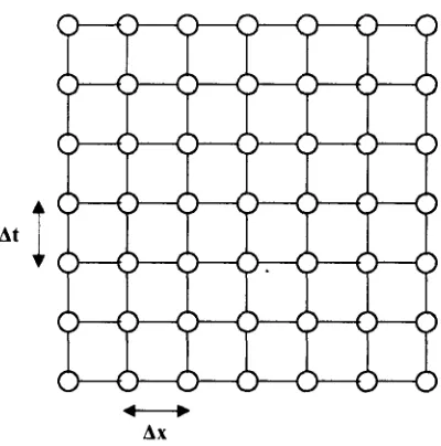
Figure 3-1 Mesh representing a one dimensional rod through several time steps 43

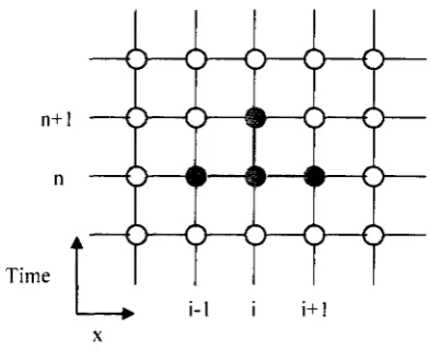
Figure 3-2 The finite Difference nodes associated with the simple explicit method 51

Figure 3-3 The finite Difference nodes associated with the simple implicit method 54

Figure 4-1 The 2-D finite difference nodes associated with the simple explicit

scheme 69

Figure 4-2 The GUI screenshot 78

Figure 4-3 Flash Method. Temperature vs. Time at the rear surface.

Heater Temperature: 373 (K), Thermal diffusivity: 10e-8(m2/s)

Figure 4-4 Thermal Diffusivity from Flash Method vs. Thickness, (red: a/;black: ec?) 81

Figure 4-5.a Thermal diffusivity vs. Pulse duration (red: a.\, black: 012) 82

Figure 4-5.b Thermal diffusivity vs. Pulse duration for the half time method 82

Figure 4-6 Experimental instrumentation 85

Figure 4-7 The relav system (Left), The Epoxy+T^o samples (Right)

86

Figure 4-8 The snapshot of the infrared camera record 87

Figure 4-9 The spot on the sample defined for temperature analysis and the plot of

its temperature evaluation vs. time

o /

Figure 4-10 Schematic presentation of converting a 2-D matrix to a 1-D

array q.

(15)

Figure 4-11 Schematic representation of the coefficient matrix (A) in implicit

method, heating from the top Q9

Figure 4-12 Schematic representation of the initial matrix (B) in implicit method, 93 heating from the left side bar

Figure 4-13 Schematic representation of the initial matrix (B) in implicit method,

heating from the right side bar 94

Figure 4-14 Implicit method in 2-D, the coefficient matrix for a sample of

< A 9 6

5 x 6

Figure 4-15 The coefficient matrix representation 97

Figure 4-16 Heat propagation in a sample 98

99 Figure 4-17 Finding thermal diffusivity in fig 4-16 using Flash method

Figure 4-18 Simulation of heat propagation in a sample with the heater at the middle

of the top side

Figure 4-19 Simulation of the heat propagation with the heater at the corner 101

Figure 4-20 Heat propagation simulation for a sample with a single defect inside

Figure 4-21 (up) Heat propagation simulation for a sample with a multiple defects

inside,(down) Flash method of finding thermal diffusivity for the same . „.,

sample

Figure 4-22 Heat propagation in a 3 layered sample, the middle layer is more heat

, t. 104

conductive

Figure 4-23Heat propagation in a 3 layered sample, the middle layer is less heat

(16)

Symbols and Descriptions

Symbol Page # Description

E

h

f

c

X

L , ,b:

k

T

Mh

a

£tt,TJ

M(TS)

Mh(T)

a

(Pa

<P,

pa.0.<t>.e',(/)')

<? , ,

4>>, 3 3 3 3 3 5 5 6 6 6 6 6 6 7 7 7 7 7 7 Electromagnetic energy Planck constant Frequency

Speed of light

Wavelength

Radiance

Boltzmann constant

Temperature

Emissive power •

Stefan's constant

Emissivity

Emissive power

Emissive power of a blackbody

(17)

T( A.&,</>)

t,

p a T

c,

Ts

L

A

r 2 D* M CO t S(x) <p(x{)

A(xt)

f(f)

Ar Alr

K

h

L D (',. 8 9 9 9 9 13 13 13 13 13 15 27 27 27 29 29 29 33 33 33 34 37 39 39 39 Transmittance Transmitted flux Reflection Absorbance Transmittance Thermal contrast

Temperature of sound area

Temperature of defected area

Detectablity of thermal contrast

Depth

Defect visibility

Diffusion length

Angular frequency

time

Amplitude of the signal

Phase

Amplitude

Fourier transform of frequency

Amplitude of a square pulse

Duration of a square pulse

Fourier transform

Blind frequency

Sample's thickness

Density

(18)

T(U)

<Kx.)

r At

AY

£

40

44

51

56 Temperature at L, t

Temperature at Xj

Thermal diffusivity

Time interval

Space interval

Error in computational method

(19)

Chapter 1

1 Historical Background

1.1 Discovery of Infrared Radiation

Infrared discovery goes back to 1800 when Sir William Herschel (1738-1822),

German-born British Astronomer who is famous for discovering Uranus on March 13, 1773. He

discovered Infrared or as he phrased it, "Invisible rays" while reproducing Newton's

experience using a prism to pass sunlight through and separate white light into colors. He

measured the temperature of each color and noticed that temperature progressively

increased from the violet end to the red end of the visible spectrum. But it came to his

surprise that temperature increased further when he positioned the thermometer beyond

the red end. Further experimentation led to Herschel's conclusion that there must be an

invisible form of light beyond the visible spectrum [1].

1.2 Thermography as a NDT Tool

In many applications; from the production lines, where in situ inspection speeds up the

process, to the characterization of antique art treasures and cultural heritages, there is an

increasing demand for safety[2]. Destructive evaluations can be useful during the design

stages, but Non-Destructive Testing and Evaluation techniques (NDT&E) are helpful

inspection tools, since they allow to examine materials or components in ways that do not

impair future usefulness [3]. NDT inspection techniques though, are required to be

reliable, economical, sensitive, user friendly and fast. Moreover, the materials and

processes are constantly evolving; hence the inspection technique should be adaptable as

well [4].

Infrared Thermography (IT), among the various NDT techniques used nowadays, is

known as an attractive tool for non-contact inspections. Different thermal properties of

(20)

disbonds. etc.) are detected as thermal contrast assuming emissivity variations, reflections

from the environment and atmosphere attenuations are negligible.

Soon after its discovery, Infrared Thermography was used as a NDT tool. From the

earliest applications of Infrared NDT, was a patent in 1935 by J. T. Nicholas [5]. He used

a radiometer to verify the uniformity at which steel slabs are reheated in a steel-rolling

mill. In 1948 R. C. Parker and P. R. Marshall [6] investigated experimentally the

temperatures generated at sliding surfaces, especially between railroad wheels and the

brake blocks. The current flow in an electric power transmission line was studied by

Leslie and J. R. Wait in 1986 [7]. Infrared radiometry also made it possible to detect the

overheated components on circuit boards in 1961 [8].

In the mid 1960s when commercial infrared cameras became available, a wide range of

applications were developed continually for this non-contact, non-intrusive technique in

military, industrial, civil engineering, environmental and medical fields.

1.3 Advantages and Limitations

A thermographic survey is totally non-destructive and unlike X-rays and ultraviolet,

infrared is harmless to living bodies. It provides fast inspections (up to a few m2 at a

time) with minimal access requirements. Measurements in inaccessible areas which are

hazardous for other test methods may be done by this method. The system under study in

this method needs not to be shut down for inspection, and this not only cuts on the

expenses but also real time images enable immediate interpretation by a skilled

practitioner [9-11].

It is also important to mention some limitations to this method.

For applying this method to a large surface, a quick and uniform thermal stimulation is

difficult to achieve. For outdoor surveys, factors such as high winds, rain, standing water

on the roof. etc. may lead to thermal loss and surface cooling, thus affecting the reliability

of the interpretation. Cracks and disbands large enough to result in measurable change oi'

(21)

thermal properties are detectable in this method. Expensive tools and experience are

required to obtain and interpret the thermal images [9-11].

1.4 Fundamentals of Infrared Thermography

It is known that all bodies at a temperature above absolute zero (-273 C) emit

electromagnetic radiation regardless of their state. The energy and wavelength of the

emitted EM wave are related through the well known relation:

E = hf = ^ (1.1)

Hence the electromagnetic spectrum would look like figure (1-1).

Increasing Frequency (v)

i<>14 io22 ioM IO1* io'6 io14 in'2 IO1" lo8 IO*1 in4 io2 io° v(Hz)

I i I . I . I i i i i i i i i

y rays

400

Xrays UV JR

1

Microwave

i

FM Rad io w

i

AM ives

Long radio waves

io-"1 i o_ u io- 1 2 ur1 0 ip"8 I ;i(r* ur" i c1 io° io2 in4 io* ms X(m)

, . . - - - - " " " " ~ ~ ~ - - - - _ _ Increasing W a v e l e n g t h (?v) - »

Visible spectrum

500 600 Increasing Wavelength (K) in nm -»

700

Figure 1-1 Electromagnetic Spectrum [1]

While the visible light wavelength lies between 0.4 to 0.7 urn, thermal radiation falls into

(22)

This radiation is usually emitted from a small portion of the surface and includes a

variety of wavelengths and a distribution of energy. (Figure 1-2)

11

s

l

SPECTRAL DISTRIBUTION

DIRECTIONAL DISTRIBUTION

Wavelength

(a) (b)

Figure 1-2 Radiation emitted by a surface (a) Spectral distribution (b) Directional distribution. (Adopted from Maldague, 2001) | 3 |

As an important concept in radiometry, blackbody is explained as a perfect radiator. A

hlackbody is defined by Gustav Robert Kirchhoff (1824-1887) to be a surface that

absorbs all incident radiation of different wavelengths and directions without reflecting or

transmitting it. It also re emits this energy evenly in all directions until it is in equilibrium

with the environment. (Figure 1-3)

(23)

(a) (b)

Figure 1-3 Features of a blackbody cavity (a) absorption, (b) emission from an aperture (Adopted from Maldague, 2001) |3|

According to Planck's law, the spectral radiance of a blackbody in thermal equilibrium is

given by [12].

2hcl A'[exp(hc/AKT)-\]

^>.M^T) = —r ,7 , ! , , ^ „ W r a > - 'f f- ' (1.2)

L would be the power of the Blackbody (b) per unit surface area and per unit of solid

angel, h and K represent the Planck's constant (6.63 x 10"34 Js) and the Boltzmann's

constant (1.381 * 1023 J/K), c is the light's speed (3 x 1 0 s m/s) and T is the blackbody

temperature in Kelvin.

This equation predicts the energy radiated as a function of wavelength at temperature T.

integrating Planck's law over all wavelengths ranging from 0 to QO, the total radiant

(24)

M

h

=

af

(1.3)

known as Stefan-Boltzmann expression [12]. 0 = 5.6697 * 10"8 W/m2 K4)

1.4.1 Emission

Unlike a Blackbody, a rea/ surface does not absorb the incident radiation completely.

Emissivity is the relative amount of a real surface's thermal radiation to that of a

Blackbody under the same conditions of temperature (7^) and direction [12].

s{A.,Ts) =

M{Ts)

Mh(Ts)

(1.4)

Emissivity of a surface is a unit less parameter that changes between 0 for a whitebody

(perfect reflector) and 1 for a blackbody (perfect emitter). Figure (1-4) shows the spectral

distribution of a real surface in comparison with a blackbody.

Blackbody, T -Real s u r f a c e , T

Figure 1-4 Comparision of a blackbody and real surface distribution of radiance | 3 |

(25)

1.4.2 Absorption

The traction of the incident flux absorbed by the surface is called absorbance.

«'%>• (1.5)

Same as emissivity, absorbance is also dependent on the incident wavelength and

direction; however it is not affected by the temperature of the surface.

1.4.3 Reflection

Reflection is defined as the ratio of the incident radiation reflected by the surface and is

affected by the direction of both incident and reflected flux [12].

P(A,ej,e',<t>') = ^L±L (i.6)

This formula is not very convenient to work with, since for a given incident radiation, the

reflection in all directions should be considered. Hence in practice surfaces are

considered either to be isotropically diffuse or perfectly specular. As is depicted in figure

(1-5), an isotropically diffuse surface reflects the incident radiation uniformly in all

directions regardless of the incident radiation and a perfectly specular surface reflects the

(26)

Incident ray Radiation of uniform i - - ^ radiance

e = e i

Incident ray j Reflected ray

ia) JbL

Figure 1-5 Reflection (a) isotropically diffuse, (b) perfectly specular (Adopted from Makiague, 2001) |3|

1.4.4 Transmission

To define transmission for a semitransparent object, the possible scattering and

absorption by the particles inside should also be taken into account. That's why it is not a

simple problem. However on a macroscopic scale, transmittance is defined as the ratio of

the transmits flux in all directions to the directly incident flux [12].

T(A,0,t) = d<t>i,t (1.7)

It is also possible to integrate transmittance over all possible wavelengths (/: 0—+oo), and

that would be called the total directional hemispheric transmittance. (Figure 1-6)

(27)

Incident Rav 0

Semitransparent Medium

Transmitted flux

Figure 1-6 Transmission process illustrated as a directional irradiance

1.4.5 Energy Balance and Krichhoff s Law

Incident radiation on a semitransparent material is partly reflected by the surface and the

rest is either transmitted through the object or absorbed by it. However, as shown in

figure (1-7), the net flux should remain unchanged.

# • = £ + & + & (1.8)

Integrating equation (1.8) over all possible wavelengths and similar directional

conditions, properties expressed previously will be related as:

p + a + T = 1 (1.9)

For opaque objects (t = 0). (1.9) becomes:

(28)

Krichhoffs law relates absorption and emission for a blackbody [12].

s (k, 9', cp') = a (X, 0. <p) (1.11)

Although equation (1.11) only applies to a blackbody, it can still be used for a diffuse

surface for which emission and absorption are independent of spectral and directional

conditions [12]. For thermography inspections black painting is used to increase

emissivity and also to prevent reflections from environment.

Incident Reflection 4>i <«>r

Figure 1-7 Flux exchange in a semi-transparent medium

1.5 Differ en t Approaches: A dive, Passive

In order to investigate a structure with Infrared Thermography, there are two approaches

that can be used, passive and active. In the passive approach, the specimen and the

ambient are naturally at different temperatures (usually the specimen is at higher

temperature). While in the active approach, an external excitation source, such as heating

or cooling system needs to supply the thermal contrast between different parts of the

sample.

(29)

1.5.1 The Passive Approach

The passive approach is commonly used for civil engineering structures inspection,

maintenance, medicine and property evaluation. The material under investigation is

usually examined for abnormal temperature profile indicating an irregularity or possible

defect, void, etc.

In passive thermography, the key word is the temperature difference with respect to the

surrounding, often referred to as the "delta-T" or the "hot spot." A delta-T of 1 to 2 °C is

generally found suspicious while a 4°C value is a strong evidence of abnormal behavior

[10]. however there have been more sophisticated applications of this approach rather

than only qualitatively pin down the anomalies. These investigations are more

complicated and need thermal modeling.

For instance in a reported application [15], a numerical method was developed to

simulate the heating process of needles used to sew fabrics in the automobile industry.

(Seat cushions and backs, airbags, etc.) The friction between the needle and the fabric

(usually synthetic) in high speed sewing generates heat which will cause worn or broken

thread and damages the thread as well as burns the fabric and weakens the needle itself.

Experiments on the plant floor have shown the temperature raise of up to 100-300°C with

the sewing speed of 1000 to 3000 rpm.

The model uses different factors such as needle design, thread fabric properties and

sewing speed to predict the temperature distribution in the needle during the sewing

process as well as the time needed to reach a steady state. By understanding the heating

process, they can reach the optimized operation through changes in needle geometry,

(30)

1.5.2 The Active Approach

Unlike the passive approach, in the active infrared thermography the characteristics of the

stimulus is known and that makes it possible to get quantitative results such as the depth

of a possible defect, hence it's widely used in NDT&E. Depending on the different

methods of data acquisition and data processing, various active thermography approaches

has been developed.

1.5.2.1 Pulsed Thermography (PT)

In Pulse Thermography, the object surface is being stimulated by a heating pulse and the

data acquisition is performed by monitoring the temperature evolution of the surface after

it starts to cool down. Lamps, flash lamps, scanning lasers or hot air jets are the most

popular heating tools and Infrared cameras are used to monitor the signal in the transient

area. There are two possible modes of data acquisition in PT. Reflection mode and

Transmission mode. In the Reflection mode, the heat source and the Infrared camera are

both placed on the same side of the specimen while in the transmission mode, the camera

faces the back surface of the sample. Reflection mode is preferred in cases where the

defect is closer to the heated surface or the rear surface is not accessible. The signal

received by the IR camera (Thermograms) is then being processed to estimate the

characteristics of the subsurface defect such as size, depth and thermal resistance.

Cielo in 1984 was the first who came up with the idea of pulsed approach [16]. He

applied this technique on the aluminum coating plasma sprayed on aluminum substrates

with artificial defects between the coating and the substrate. The parameters of interest

were the thickness, adhesive and cohesive strength. In order to interpret the experimental

results, he developed a numerical model based on the inversion procedure and got

encouraging results.

In ll)85. for the first time Balageas et al. developed an analytical model using finite

difference method to study the thermal decay in a coated substrate [17]. Given the

(31)

thermal properties and the thickness of the substrate, the model could evaluate the

thermal properties and the thickness of the coating and the thermal contact resistance of

the interface. Cielo and Krapez used this technique to remotely measure the thickness of

oil film on water. They could evaluate the oil thickness up to 1 mm with the error range

of 0.1 mm [18]. However, there are some practical limitations in adopting this method for

open-air environmental applications. The problems could rise by the energy absorption of

the laser pulse by the atmospheric aerosols or the oil film immerging into water.

One of the problems with thermal images developed by PT was the blurring. It was

assumed that loss of information during the data acquisition was the cause of blurring,

however in 1992, Favro et al [19] could remove the blurring by developing an algorithm

which performs a mathematical inversion of the scattering process to the experimental

data. As proved by Vavilov (1992) [20], the reverse method will predict more than one

combination of defect characteristics for a single thermogram. Thus, it was suggested that

the iterative calculation should be done knowing some of the defect's parameters, a priori

beforehand [21]. However, these methods turned out to be time consuming and only

applicable to some specific cases.

The difference between the thermal properties of the defected and non-defected (sound)

areas causes the thermal contrast which is measured and evaluated in PT.

The larger the thermal contrast, the more detectable the damaged area. Cr not only

changes by different atmospheric conditions and the device precision, but also is affected

by the size and depth of the defect. Smaller defects and deeper-located ones will result in

lower thermal contrast, hence harder to evaluate. It is understood that the loss in Cp is

proportional to the cube of depth:

(32)

Maldague (2002) [22] suggested to use a rule of thumb that says the radius of the smallest

detectable defect should be at least one to two times larger than its depth under the

surface.

To study the limits in defect evaluation by infrared thermography, Meola et al ran a

thorough experiment on composite specimens with external material as defects [23].

Results proved the key role of the thickness in defect visibility, meaning that a thin large

defect is more difficult to detect than a thick small one at the same depth.

However, there are a few drawbacks in these computational approaches leading to some

inaccuracies. One of such was the fact that not always a priori parameter of the defect

was available. Also the sound area was assumed to have evenly distributed temperature

over the surface.

In 2002, Pilla et al [24] solved the one dimensional Fourier equation assuming a Dirac

pulse applied to a homogeneous semi-finite plate:

AT = -T£=~ (1.14)

•sjnpCk y/t

In this equation, Q is the total energy absorbed and yjpCk is called thermal effusivity

(e). This equation defines the temperature of sound area locally as a function of time.

Hence the variation of effusivity with time is studies to evaluate the depth and thermal

resistance of the defect zone.

This approach brought some distinctive advantages to PT by introducing the New

Absolute Contrast (NAC) based on the reconstruction of the temperature in the sound

area [24].

(33)

Since thermal contrast is evaluated based on the total energy (Q) and Q is affected by

non-uniform heating and convection, Peng and Almond (1998) [25] proposed to replace

it with defect visibility.

The subscripts d and s represent the surfaces above the center of the defect and the sound

area.

Although pulse thermography is the sufficient choice in many applications, it is affected

by the local variation of the emissivity coefficient and non-uniform heating that can mask

the defect visibility. The emissivity problem may be solved by painting the surface, but

this could be a solution only for parts where this surface finish is allowable [21].

Various methods based on different stimulating or processing techniques are being

reviewed in the following sections.

1.5.2.2 Lock-In Thermography (LT)

Heat injection during the short time of a pulse (e.g. typically 10 ms for a powerful flash

lamp) may cause initially high temperature on the surface. Another surface heating

method is by modulated heat deposition in which energy is distributed over a longer

period of time. Therefore it reduces the thermal load of the inspected component to a

power density which is typically below the one of sunshine at noon in summer [26].

The basic idea in modulated or Lock-in thermography (LT) is submitting the specimen

under study to a periodic (sinusoidal) temperature stimulant. In this case, highly

attenuated and dispersive waves will form inside the sample and they are known as

"thermal waves" [10]. Like all other waves, thermal waves reflect from the boundaries

(34)

and phase of the sinusoidal wave pattern at each point which can be used to evaluate the

temperature variation. The phase image can be used to directly specify not only the size

but also the depth and thermal resistance of any kind of imperfection in a sample.

Carlomagno and Berardi came up with the idea of modulated thermography in 1976 [27].

Further investigation to utilize NDT of materials with this method was done by Beaudoin

et al (1985) and Kue et al (1992) [28, 29]. In 1994, Busse et al used LT for depth

profiling of fiber orientation in composite laminates [30]. Since then LT has been used

for defect detection in veneered wood (Wu 1994) [31], measure thickness, density and

porosity of ceramic coatings (Wu et al 1996a, Rantala et al 1996) [32, 33] and inspection

of aircraft components (Wu et al 1996b 1998) [26, 34].

Meola and his group (2002, 2003, 2004) [35-40] at the University of Naples investigated

in the capability of this method to deal with other applications such as measurements of

material thermal diffusivity, evaluation of assembly ways like adhesive bond joints, as

well as control of bonding improvements after surface plasma treatment.

For a thermal wave modulated at frequency co, the thermal diffusion length is given by

this relationship:

M = M (1-16)

Where a is the thermal diffusivity of the material and the wave frequency is / = (O/2TI.

While u is the maximum depth range in amplitude image, the maximum thickness that

can be inspected in a phase image is proved by Busse and Rosencvvaig (1980) and Busse

(1982) [41, 42] to be:

/; = l-8ARr (1.17)

(35)

Hence the penetration depth of thermal waves in the material depends on the properties of

the material (heat conductivity, heat capacity and density) as well as the wave cycle time.

The slower the wave, the deeper it can penetrate in the material. To start a test, usually

one would start to investigate the surface layer using high frequency waves, then

reducing the frequency to observe deeper layers until the whole thickness is examined.

From limitations of this approach, one is the low frequency range needed for

investigation of thick materials with low thermal diffusivity which not all the heat flux

modulators can provide. Also it is possible to miss a defect because of not choosing a

proper frequency. In practice lock-in thermography is rather time consuming for

evaluation of thick materials with low thermal diffusivity.

More recently in 1999, Dillenz et al used an ultrasonic transducer attached to the sample

[44]. Their method has the advantage of selective heating of only the damaged area, and

is proved to detect deeper and smaller defects. From the applications of this method are

detection of corrosion, vertical cracks and delaminations. In the next section a

combination of the previous methods named Pulsed Phase Thermography (PPT) is

described.

1.5.2.3 Pulsed Phase Thermography (PPT)

The idea behind Pulse Phase Thermography is to combine two previous methods in a way

that enables us to make use of the advantages of PT and LT while avoiding their

drawbacks. Data acquisition in Pulse thermography is fast and straight forward while in

LT, more specialized equipment is needed plus the experiment is rather time consuming

in LT. On the other hand, the data in PT is highly affected by thermal, optical and

geometrical surface characterizations and the environmental reflections, while using the

phase images to process the data in LT makes it less sensitive to these conditions.

(36)

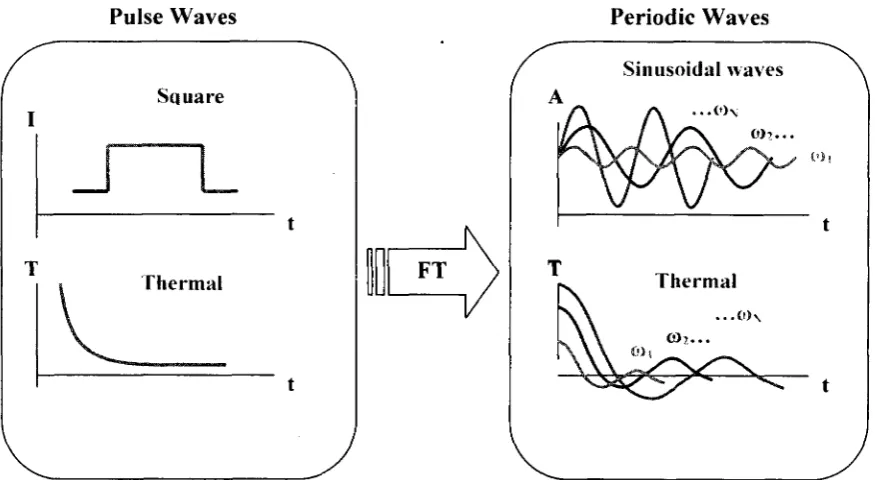
frequencies. (Figure 1-8) Based on this theory, in PPT as in PT. the sample is pulse

heated, yet the Fourier transform on the temporal decay wave in the specimen

unscrambles the mix of frequencies in each pixel. So that, a phase or magnitude image of

each pixel is provided as in Lock-in Thermography.

Pulse Waves

S q u a r e

J L

T h e r m a l FT

Periodic Waves

Sinusoidal waves

. . ( 0 \

Figure 1-8 Pulse thermography vs. Lock-in thermography (experimental configuration)

Historical Notes on Pulsed Phase Thermography

Pulse Phase approach was introduced by Maldague and Marinetti in 1996 [44]. Maldague

and his group kept working on this method and reported their progress and results on its

application. Given the non- linear and noisy character of pulsed thermographic data,

inverse solutions are difficult to reach, that's why PPT was only used as a qualitative

defect detection approach for the first couple of years from its discovery until in 1998.

Maldague and his group tried to get quantitative results using neural networks [46|.

Neural network approach was chosen due to its ability to work with non linear problems

with missing or noisy data. Although this approach opened new windows to quantitative

(37)

investigations in infrared NDT, high sampling frequency was needed for the data

acquisition system, depending on the material's thermal diffusivity.

A practical drawback of Fourier Transformation is the infinite extensions on time axis of

the basis function which causes information loss on the time evolution of the spectral

properties of the signal. The time information is needed for defect depth retrieval, so

another transform rather than Fourier Transform is needed. In 2000, Maldague et al

adopted wavelet transform for signal processing [47]. This method provided the

frequency analysis without missing on time information. However, the last two

approaches proved to be too lengthy in computational routines to be applicable in most

NDT processes. Later in 2004, they proposed a new depth retrieval approach based on

absolute phase contrast defined as [48].

A(p=<pd'-(ps (1-18)

Where the subscripts d and s stand for the defect and sound areas. They proved that the

depth changes with the blind frequency (fb), frequency at which a defect generates enough

phase contrast to be invisible, as:

zKafb1/2 (1.19)

They also tested their theory on Plexiglas and Aluminum, two materials with low and

high conductivity and the results well agreed with the theory [48]. Following this work,

steel plates with flat bottomed holes were studied by this group in 2005 [49]. The defects

were located at different depths ranging from 1 to 4.5 mm and the results showed the

same correlation between the blind frequency and the defect depth.

PPT has proved to have a great potential for NDT applications and investigations on its

(38)

1.6 Instrumentation for Infrared Thermography:

When it comes to experimental analysis, the set up and instrumentation is of great

importance. This is an overview of investigation tools, such as detectors, radiometers,

infrared cameras and a brief review of the methods to apply various thermography

techniques and data acquisition.

1.6.1 Detectors

Optical receivers are the main part of infrared radiometry systems. As of 1999, the

worldwide IR detector market was estimated to be $10 billion increasing by rate of 30%

every year [51]. An infrared detector or sensor is used to convert the radiant energy to

some other assessable quantity such as the electrical signal. There are two types of

sensors: thermal detectors and photonic detectors.

1.6.1.1 Thermal Detectors

In thermal detectors, the incident radiation raises the surface temperature which changes

the electrical conductivity of the heated material and in turn affects the output signal.

Thermal detectors response is independent of incident wavelength and this characteristic

makes it unique in this way. To discuss the sensitivity of thermal detectors, one should be

familiar with effective conductivity GR which is given by [52]:

GR=4o?A (1.20)

Where T represents the sensor temperature, a is the Stefan-Boltzmann constant, and A is

the detector-sensitive area. Then the detectivity limit is [51 ]:

£ * = , — V ~ (1-21)

V 4kT2G

(39)

k is the thermal conductivity and G is the limit of GR.

Depending on the physical property affected by the surface heating in the thermal

detector, there are different types of thermal detectors.

Bolometers, are the ones in which the electrical conductivity is the changing factor.

Thermopiles are made from many thermocouples connected in series or in parallel.

Temperature difference generates voltage difference in each thermocouple through

Thompson effect. The signal in Pneumatic detectors is generated by pressure variation of

a definite volume of gas. Another type of thermal detectors is Pyroelectric detectors that

make use of the Pyroelectric crystals. As introduced in 1984 by Granicher, temperature

change in Pyroelectric crystals produces electric polarity [52]. Temperature variation in

the detector's surface Pyroelectric crystals causes the charge variation and thus a transient

current to be picked up. Liquid crystals are also used as thermal sensors. When

illuminated by white light, they reflect color light from red to violet under temperature

changes providing the resolution of up to 0.01 °C [50].

1.6.1.2 Photonic Detectors

In Photonic detectors, incident photons on a semi conductor material will generate

excitation which is directly measured by the detector. The incident photons on

photocathode will pull away electrons from the valance to the conduction atomic band.

This method prevents unnecessary heating of the sensitive surface. There are two types of

photonic detectors: photoemissive and quantum

In photoemissive photonic detectors, the current (electron flow) will generate the

resulting signal while in quantum detectors either the change in conductivity or the

generated voltage is being measured. Since there is no heating involved in this process, it

is much faster than thermal detectors and the use of solid state material allows these

(40)

1.6.2 Infrared Imaging Instrumentation

In order to get one or two dimensional images from the detector, there are two main

approaches: using a single detector attached to an electromechanical scanning device, or

using an array of individual IR detectors with no movement applied (Focal Plain Arrays).

Since first introduced in 1973 by Shepherd and Yang [53], large arrays of 512 x 512 has

been produced by different companies and they are the most popular IR imaging tools in

today's technology. An infrared camera is made of FPA, the appropriate optics and

electronics and cooling system. There are two readout tools for the FPA, Charge Coupled

Device (CCD) and Complementary Metal Oxide Semiconductor Device (CMOSD).

CMOSD is less expensive than CCD and enables windowing (reading a section of the

array rather than the whole data) however; it has higher noise and less sensitivity. In

today's applications, CCD leads the scientific and technical field while CMOSD is being

employed in the applications such as surveillance, camcorders, snapshots, etc.

1.7 Summery

In this chapter, basic and practical concept of infrared thermography was reviewed. Also

a brief review on various NDT applications for IR thermography since its discovery was

presented. Pulse thermography and lock-in thermography as two main methods in IR

thermography and their advantages and drawbacks were described. As a conclusion,

pulse phase thermography, as a combination of both Pulse Thermography and Lock-in

Thermography was found to benefit the advantages of both methods without sharing their

imperfections.

In the imaging process, thermal and photonic detectors are explained based on their

method of converting the thermal variation of the surface to an electric signal. For further

signal processing, two types of devises (CCD and CMOSD) are used for different

applications. The next step in IR thermography would be image processing methods

which will be reviewed in the next chapter.

(41)

Chapter 2 2 Thermography Techniques

In this chapter, the main principals of heat propagation in a material are presented as well

as different numerical solutions to the heat equation. Mathematics of various image

processing methods in IR thermography is discussed to prepare for the logic behind the

algorithm developed in the next chapter.

2.1 The Heat Equation

The one dimensional heat equation is [55]:

dT(x,t) d2T(x,t) n , „ ,„ „

—y- ^ - = a V - ^ 0<x<L, t>0 (2.1)

dt dx~

In this equation, a = k/pc is the thermal diffusivity and is a property of the material with

k, p and c being heat conductivity (W.m"'.K"'), density (kg.m"3) and specific heat (J. kg"1.

K"1). T is the transient heat function in a semi-infinite material with thickness L.

This equation can be solved both for a pulse or periodic thermal waves.

2.2 Pulse Thermography (FT)

Pulse thermography is a popular method in IR thermography in which the specimen is

pulse heated and the temperature decay is recorded. Assuming the heat pulse to be perfect

Dirac delta function (in practice however, a pulse with very short duration is used), the

(42)

T{z.t)=T0 + O

exp(-4at (2.2)

In this equation, z represents the depth and O is the energy absorbed by the surface [J/trr]

and To is the initial temperature [K].

To study the temperature behavior at the surface (r=0), Eq. (2.2) becomes:

r(o,/) = r

0

+-

Q e^M

(2.3)

e being effusivity and defined as Jkpct

2.2.1 Data Acquisition in Pulse Thermography

A typical experimental setup for active thermography is illustrated in figure (2-1). First

the thermal pulse is sent to the specimen's surface. Second an infrared camera records the

thermal decay of the surface. The heat source and the camera are either placed on the

same or opposite sides of the sample depending on the inspection method

(Reflection/Transmission) selected.

Kciii.

^vr-uLroiu/mior |

• • » '

m

Ti

L J

IJUUUUB

ik C'ii;:u-J

Fi«ure 2-1 Experimental setup for active (optical) thermography by Transmission or Reflection mode, source: http:/Av\v\v.visiooimage.com

(43)

The data is then recorded in 3D matrices, containing both spatial (x-y coordinates) and

temporal (i coordinate) information. To process the data there are two options of (1)

working at pixel level which is the temperature changes of a fixed point in space through

time or (2) at 2D images or thermograms which are the temperature profile of the surface

on time domain. (Fig. 2-2)

X

1

o

,V

ti t2 tN

t

Figure 2-2 Thermograms on the time domain, it is also possible to study the temperature behavior of pixel (i,j) through time.

2.2.2 Defect Characterization

The temperature profile of a sample can be used for subsurface defect detection purposes.

After the heat pulse is employed on the sample's surface, it reaches the subsurface layers

and drops quickly due to diffusion and also radiation and convection losses. However, a

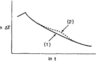
defect under the sample's surface will reduce the diffusion rate. Figure (2-3) illustrates

the temperature decay curves of two samples of the same material with and without a

subsurface defect. They behave similarly the first instants after the heat pulse is applied,

however as soon as the heat front reached the defect area with different ejfusivity. the heat

exchange rate with environment changes hence the difference in temperature above the

(44)

In AT

In t

Figure 2-3 Temperature evolution curve after absorption a rectangular heat pulse: (1) plate made of homogeneous material; (2) same plate containing a subsurface flaw (From Maldague, 1993)

This allows finding temperature contrast which is defined as:

C(t) = TM(t)-T hl(t) (2.4)

Thermal contrast is the base of many defect detection analyses. Some methods employ

the time and temperature at which the maximum of the peak is located for each pixel

(figure 2-4), to reconstruct Maximum Contrast timegrams or thermograms. Also half the

time of maximum of thermal contrast curve [57] and the slope of the curve [58] have

been used to indicate the size, depth and thermal resistance of the defect.

0.9 0.8 0./

0 6 0 5 0 4 0 3 0 2

0.1

0 0

25 30

(45)

This method provides good results as long as the sample is homogenous with fairly

shallow defects. Moreover, non-uniformity in heating process is practically inevitable,

which makes the thermal contrast curve difficult to interpret.

2.3 Lock-in Thermography (LT)

In Lock-in thermography (LT), instead of a heat pulse, modulated heat is generated by

the heat source and delivered to the surface. The input modulated wave is defined by its

angular frequency co and its magnitude / , the thermal wave generated in the sample will

propagate at the same frequency but different amplitude (A) and also a shift in the phase

value (</>). (Figure 2-5)

Input |l,«| Output |A.co.ipl

r \ I \

\J \j t <t> \J \J t

Figure 2-5 Input/ output modulated wave in lock-in thermography

The one dimensional solution to Eq. 2.1 for a modulated heat source is expressed as [60]:

T(iJ) = T0e\p(-~ )cos ITVZ

A at (2.5)

It is assumed that the thermal wave is propagating in a homogeneous semi-infinite

material where Ttl is the temperature of the surface right after stimulated by the source

(46)

a is thermal diffusivity of a material and expressed as [60]:

k,p,cp are thermal conductivity, density and specific heat.

2.3.1 Data Acquisition in Lock-in Thermography

Lock-in thermography has the advantage of not being a point by point imaging process.

In the conventional thermography methods, a laser beam would stimulate the surface at a

certain point and the detector would pick up the locally generated thermal wave from the

same point. The Fourier analysis is then to be performed on the read out signal to provide

the amplitude and phase information of that point. One drawback to the point by point

scanning process is time concerns. The measurement time should be long enough to

cover one complete modulation cycle at minimum; for instance, it would take 5 seconds

for a thermal wave with frequency of 0.2 Hz to complete its cycle. Now this should be

multiplied by the number of pixels (usually as order of 10? pixels) to obtain the total data

acquisition time. This approach could take so long for a large sample that makes it

inapplicable to the industry.

(47)

However, this problem would be solved by using an extended heating source instead of

the point heating [59]. Also it is possible to employ an infrared camera as a thermal

detector array. A Fourier transform should be performed on the signal from each pixel to

get the magnitude and phase of the modulation.

One concern is that the process should not take longer than the data acquisition itself. In

1998, Wu and Busse [59] found that the process would be particularly fast and easy using

a sinusoidal heat injection.

2.3.2 Establishing Phase and Amplitude Information

Lt works on the base of stimulating the sample's surface by modulated heat and

observing the temperature variation over the surface to reconstruct the responding

thermal wave. In case of a sinusoidal heat injection, the temperature field is also a sine

wave which can easily be recovered from three or four data points in a modulation cycle.

As shown in figure 2-6, the reference signal is reconstructed from 4 equidistant data

points, Si (i = 1 to 4) being the detector signals at pixel xi. The Amplitude A and phase <p

are [59].

<p(x,) = arctan S,(s,)-S,(s,)

S2(*,)-S4(x,X

(2.8)

(48)

Figure 2-6 Computation of phase, amplitude and thermographic images in LT. During each heating cycle, the infrared camera takes four images (Top) local thermal waves are reconstructed for any pixel (Busse, 1994)

As it is clear from equation (2.8), phase image is less affected by inhomogeneous

illumination, surface emissivity variation [59] or the reflection from the environment

[61]-Although the image can be recovered by only four data points, in practice one would

prefer to work with different modulation frequencies which would fit more than four

points in a complete cycle. Moreover, working with more data points will reduce the

noise. In that case, as shown by Wu in 1996 [62], all points in one 90°-interval can be

averaged to 1 point which is the corresponding 5, in equations (2.8) and (2.9). (Fig. 2-7)

(49)

Excitation 1024 Thermography 4 averaged thermo-images graphy thermo-images S1....S4

Figure 2-7 Reconstructing the thermal wave in LT from 1024 data points (Wu, 1996)

Finally other than the modulated heat injection, a lock-in apparatus is similar to that of

pulse thermography. (Figure 2-8)

IR-camera

HL.

Sample Thermal wave source

»<8*ar"i

Phase image

Lock-in module

Control unit

(50)

2.4 Pulse Phase Thermography (PPT)

2.4.1 Theory

Pulse phase thermography (PPT) is in fact a combination of the two previously described

Lock-in thermography and Pulsed thermography methods. PPT utilizes the time

frequency duality to extract phase images from PT results using Fourier transform, the

well known mathematical formulation in transform analysis.

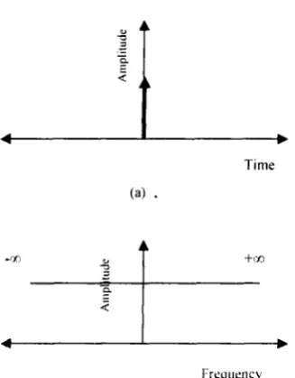
In theory, an ideal Dirac pulse of null duration can be transformed to a flat distribution

over frequencies ranging from -oo to +00 in the frequency domain. (Figure 2-9)

Time

(a)

-<x

•4

tud

c

Amp

l

i

_

i.

+QO

- > • Frequency

Figure 2-9 Time frequency duality (a) an ideal temporal pulse of zero duration and infinite amplitude and (b) its frequency spectrum

(51)

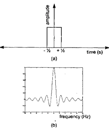
However, in practice the thermal pulse used is different from an ideal Dirac pulse in the

sense that it has finite amplitude and duration values. As an example, one can consider a

square pulse with amplitude Ap and duration AT centered on t = 0. (Figure 2-10) The

corresponding frequency spectrum would be defined by Fourier transform [50].

W ) =

A Atrsin(7ifAt ) ApAtp sinc(7fAtp) (2.10)

The shape of F as a function of frequency would look like the graph in figure 2-11, which

proves that unlike an ideal Dirac pulse, here a finite frequency range is involved in the

frequency domain, each appearing with various amplitudes.

* A

a

E

- y2 + y*

0)

time (s)

frequency (Hz) (b)

(52)

2.4.2 Data Acquisition in Pulsed Phase Thermography

In Pulsed Phase thermography, after the sample surface is stimulated by a heat pulse,

temperature evolution of the surface is recorded in N thermogram sequences. Observing

the behavior of a single pixel (i,j) during N recorded thermograms will provide a vector

T(k) where k is ranging from 0 to N-l. (Figure 2-11) Amplitude and phase images can

be extracted from this vector using a discrete one-dimensional Fourier transform [51].

Fn = J^T(k)e\p(2mkn/ N) = Re(F„) + /Im(F„) (2.11)

A=l

In this equation n stands for the frequency increment in the frequency domain.

3-, infrared image sequence L (after thermal pulse)

• Fourier Transform of temperature evolution • Computations of Ren, lmn

• Computations of phase, amplitude

Figure 2-11 Temperature evolution of pixel (i,j) through N thermograms

(53)

Establishing Phase and Amplitude in Pulsed Phase Thermography:

The imaginary and real parts of equation (2.11) are then used to extract the amplitude and

phase images [51].

A„ =^JRe;+lm; and 0n=atan

Re„ (2.12)

This process is repeated for every pixel on the surface until the ampligrams and

phasegrams for all the frequencies in the frequency domain is reached [63]. (Figure 2-12)

f. u

Figure 2-12 (Left) Amoligram and (Right) Phasegram sequence in the frequency domain

For a typical non-defective pixel like (i,j), the amplitude and phase profile would look

like figure (2-13) [63].

(54)

It can be seen from figure (2-13) that a sequence of N thermograms will provide N/2

useful frequency components and the other half can be predicted due to the odd/even

nature of the profiles.

The advantage of working in frequency domain is that the phase images are much less

sensitive to problems such as non-uniform heating, reflections from environment, and

emissivity variations in the surface. Also as compared to LT, this method has the

advantage of getting a complete phase profile from a single run.

2.4.3 Defect Characterization in Pulsed Phase Thermography Using Depth Inversion

Once the data acquisition is done, the phase contrast profiles will be employed to find the

defect's depth. Figure (2-14) shows the phase profiles of two flat bottomed holes in a

sample located at different depths z/ and z?. Considering zs as a sound area in the same

sample, the phase contrast profiles for each defected pixel is calculated

using A^ = <f>d -<f>s. As depicted in figure (2-14), phase contrast profiles have non-zero

values from /=# to a specific frequency names blind frequency (f), which has a different

value for each pixel. Blind frequency is defined as the first point in frequency domain

(while moving from higher frequencies to lower ones) at which the phase contrast is

visible for a defect. In fact blind frequency for a pixel is the point on its phasegram where

it merges with the phase profile of a sound area. As a result, deeper defects have lower

blind frequencies (fh_ > fh,, )•

-Jt)|rad| s'—^Oz,

/.-..JO.-X

• V o?tf>_ ••••

iMia.il I

36 Figure 2-14 Depth evaluation with phase contrast and

blind frequency

lb.:.

Sixvmion

(55)

Once the blind frequency is found for a defect zone, the depth z is proved to be related to

it as follows [63].

= C,I^

+

C (,,3)

Where a = kl pcp is thermal diffusivity. As this term is used to fit experimental data, C|

and C? are found to be around 1 and 1.5 respectively [63].

2.5 Thermal Diffusivity

Thermal diffusivity is a significant property of a material that establishes the rate of

transitory heating and cooling and is defined as:

cc = — (2.14)

Where k, p and c are thermal conductivity, density and specific heat.

Measuring a is of great importance to researchers for various reasons. Knowing the

thermal diffusivity of a material makes it possible to predict the heat pulse behavior in it,

as well as investigating the subsurface defects and composition.

2.5.1 Diffusivity Measurement

Different techniques have been developed over time to measure the thermal diffusivity of

a material. Non-contact measurements involve a transitory excitation delivered to the

Non-destructive investigation of thermal diffusivity in a layered material using finite difference modeling

Scholarship at UWindsor

Scholarship at UWindsor

Non-destructive investigation of thermal diffusivity in a layered

Non-destructive investigation of thermal diffusivity in a layered

material using finite difference modeling

material using finite difference modeling

Non-destructive Investigation of Thermal Diffusivity

in a Layered Material Using Finite Difference

Modeling

By

Ghazal Ghodsi

A Thesis

Submitted to the Faculty of Graduate Studies

Through the Department of Physics

in Partial Fulfillment of the Requirements for

the Degree of Master of Science at the

University of Windsor

Windsor, Ontario, Canada

2010

1*1

• + •

Author's Declaration of Originality

ABSTRACT

To my one and only: Kiyan

ACKNOWLEDGEMENTS

TABLE OF CONTENTS

LIST OF TABLES

LIST OF FIGURES

Symbols and Descriptions

Symbol Page # Description

t,

c,

L

A

f(f)

K

h

40

44

51

51

51

56

Temperature at L, t

Temperature at Xj

Thermal diffusivity

Time interval

Space interval

Error in computational method

1 Historical Background

1.1 Discovery of Infrared Radiation

1.2 Thermography as a NDT Tool

1.3 Advantages and Limitations

1.4 Fundamentals of Infrared Thermography

11

l

M

=

af

1.5 Differ en t Approaches: A dive, Passive

1.5.1 The Passive Approach

M = M (1-16)

J L

1.6 Instrumentation for Infrared Thermography:

1.6.1.2 Photonic Detectors

1.7 Summery

Chapter 2

2 Thermography Techniques

2.1 The Heat Equation

2.2 Pulse Thermography (FT)

r(o,/) = r

+-

m

Ti

L J

2.3 Lock-in Thermography (LT)

2.3.1 Data Acquisition in Lock-in Thermography

HL.

2.4 Pulse Phase Thermography (PPT)

**1*1**