INVESTIGATION
How Population Growth Affects
Linkage Disequilibrium
Alan R. Rogers1 Department of Anthropology, University of Utah, Salt Lake City, Utah 84112 ORCID ID: 0000-0003-3987-3346 (A.R.)
ABSTRACTThe“LD curve”relates the linkage disequilibrium (LD) between pairs of nucleotide sites to the distance that separates them along the chromosome. The shape of this curve reflects natural selection, admixture between populations, and the history of population size. This article derives new results about the last of these effects. When a population expands in size, the LD curve grows steeper, and this effect is especially pronounced following a bottleneck in population size. When a population shrinks, the LD curve rises but remains relativelyflat. As LD converges toward a new equilibrium, its time path may not be monotonic. Following an episode of growth, for example, it declines to a low value before rising toward the new equilibrium. These changes happen at different rates for different LD statistics. They are especially slow for estimates ofs2
d, which therefore allow inferences about ancient population history. For the human population of Europe, these results suggest a history of population growth.
L
INKAGE disequilibrium (LD) refers to the statistical as-sociation between pairs of genetic loci. It is used routinely in localizing disease genes, in detecting natural selection, and in studying population history. In all of these contexts, it is necessary to account for effects of changes in population size.These effects arise because inhabitants of small popula-tions tend to be close relatives. The genealogical paths that separate them are short, and this reduces the opportunity for recombination. For this reason, LD rises after a fall in population size and falls after a rise.
These effects are understood in a general way and are often studied by computer simulation (Kruglyak 1999; Pritchard and Przeworski 2001). Although this approach has led to important insights, our understanding is still rudimen-tary. This article uses a deterministic algorithm to explore the effects of growth, of decline, and of temporary reduc-tions (bottlenecks) in population size. It shows that each type of history leaves a distinctive signature in the “LD curve,”which relates the LD between pairs of sites to the distance that separates them along the chromosome.
The paper uses s2
d(defined below) as a measure of LD.
This choice is unusual, becauses2
dhas always been of
sec-ondary importance. As we shall see, however,s2
dhas
dynam-ical properties that give it deeper time depth than alternative measures of LD. It is readily estimated from data and can be predicted by a deterministic theory, which makes it easy to study the response to changes in population size. This article shows that s2
d is of more than secondary importance. It is
useful in its own right as a measure of LD.
Materials and Methods
Software
The various methods were evaluated against simulated data generated by MACS (Chenet al.2009). Simulation results in Figure 1 are based on my own coalescent program, hetage, written in C. All other analyses were done using ldpsiz, a package of C programs available at github.com/alanrogers/ ldpsiz. This package includes several programs: eld, which estimatess2dandr2from genetic data; preld, which
calcu-latess2
dfrom the history of population size; and sald, which fits history parameters to an observed LD curve, using the method of simplex-simulated annealing (Press et al. 1992, pp. 451–455), with modifications described by Gao and Han (2012).
Measuring LD
Consider a pair of loci (nucleotide sites),AandB. At locusA, allelesA1andA0have frequenciesaand 12a. At locusB, alleles B1 and B0 have frequencies b and 1 2 b. The
Copyright © 2014 by the Genetics Society of America doi: 10.1534/genetics.114.166454
Manuscript received November 10, 2013; accepted for publication May 28, 2014; published Early Online June 6, 2014.
1Address for correspondence: University of Utah, 270 S 1400 E Rm 102, Salt Lake City,
disequilibrium coefficient,D, is defined such thatab+D is the frequency of gamete typeA1B1. The sign ofDis arbitrary, depending on how one labels the alleles, so the magnitude of LD is often measured byD2.
These measures are sensitive to heterozygosity at the two loci, so many authors prefer the squared correlation co-efficient (Hill and Robertson 1968),
r2¼ D
2
að12aÞbð12bÞ: (1)
Unfortunately, there is no consensus regarding the expected value of this statistic, even in the simplest case of neutral loci in a randomly mating population of constant size (compare Sved 2009 with Song and Song 2007 and Durrett 2008, p. 98).
Ohta and Kimura (1969, p. 233) proposed a related mea-sure of LD, the“squared standard linkage deviation,”which was also motivated by a desire to minimize the effect of heterozygosity:
s2 d¼
ED2
E½að12aÞbð12bÞ: (2)
This measure is usually viewed as an approximation to
E[r2]. It is most useful in this role when the population size
is large and constant and both loci have appreciable hetero-zygosity (Hudson 1985). In other situations, the two param-eters can differ greatly. But even when s2
d fails as an
approximation, it is still useful as a measure of LD. This is not to say thats2
dprovides a complete
descrip-tion of variadescrip-tion at a pair of loci. That is a problem with multiple dimensions, which cannot be solved by any scalar-valued measure of LD (Weir 1996, pp. 125–127). Such mea-sures are simplifications and are necessarily incomplete (Schaperet al.2012). However, as we shall see,s2
dcaptures
enough to provide an interesting window into the history of population size.
Estimation ofs2
d
One can estimate s2
d from data by replacing the expected
values in Equation 2 with averages across the genome. For this purpose, I treat each polymorphic site [single-nucleotide polymorphism (SNP)] as“focal”and compare the focal SNP with each other SNP within some given range. From each comparison, I calculate D2 and a(1 2 a)b(1 2 b). These
values are tabulated separately within bins based on the distance in centimorgans between the SNPs. After all com-parisons have been tabulated, the estimateðs^2dÞis calculated
as the sum ofD2within a bin divided by the corresponding
sum ofa(12a)b(12b).
In this article, I ignore pairs of SNPs separated by .0.3 cM, because there is little LD at these distances in most parts of the human genome.
To estimate uncertainties, I use a moving-blocks boot-strap (Lieu and Singh 1992), with 300 SNPs per block. With diploid data, some genotypes may be unphased. In such cases, I use the EM algorithm to estimateD2, as explained
in theAppendix.
Deterministic evolution ofs2
d
Under neutral evolution with constant population size, s2 d
converges to an equilibrium value (Ohta and Kimura 1971; McVean 2002). In addition, several authors have introduced recurrence equations, which make it possible to study the transient behavior of s2
d after changes in population size
(Weir and Cockerham 1974; Hill 1975; Strobeck and Morgan 1978). The model of Strobeck and Morgan (1978) allows faster calculations but is less numerically stable than that of Hill (1975). I present some results using the former model but focus primarily on the latter. In the Appendix, I summarize Hill’s model and show that it holds not only un-der the mutational model that he studied, but also unun-der the model of infinite sites (Kimura 1969). It is thus appropriate for use with DNA sequence data.
For bootstrap confidence intervals, I accelerate these calculations by using Equation A2 of theAppendixto approx-imate a system of ordinary differential equations, which is then solved using standard software.
Sampling bias
Drawing a sample is equivalent to one generation of evo-lution with a very small population—one whose size equals that of the sample. Because drift introduces LD, there is much more LD in a sample than in the population from which it was drawn.
Hudson (1985, Equation 6) showed that sampling bias in r2equals 1/n, when the sample consists of n gametes.
Sampling bias also inflates the value of ^s2d:The program
preld includes this bias in calculations of the expected value, s2
d:These calculations use the model of Hill (1975) or Strobeck
and Morgan (1978) to project the state vector forward one generation, with the population size set equal to the sam-ple size.
Figure 1 The depth,T, of gene genealogy given heterozygosity,H. The
Fitting population history to an observed LD curve
The program eld (a part of ldpsiz) estimates the LD curve from genetic data. A second program, sald, can then be used to search for the population history parameters that mini-mize the sum of squared differences between observed and predicted LD curves. This minimization problem searches a complex surface, with many local minima. To search for the global minimum, sald uses the method of simplex-simulated annealing. For each data set, sald starts 10 simulated an-nealing jobs on parallel threads. Typically, several of these converge to the same global minimum. sald returns the best of the 10 solutions asfitted parameters.
Results
^ s2
d is average r2, weighted by heterozygosities
Equation 2 is equivalent to
s2 d¼
EHAHBr2
E½HAHB ;
(3)
where HA = 2a(1 2 a) is the expected heterozygosity at
locus A and HB is that at locus B. This implies that s2d is
the expectation of r2 weighted by the product of the two
heterozygosities.
This weighting also carries over to the estimate,s^2d;which
is obtained by replacing expectations with averages. Such estimates will be insensitive to loci with low heterozygosity and, for this reason, also insensitive to sequencing error. They should be useful with low-coverage sequence data.
Loci with high heterozygosity have deep gene trees
Weighting by heterozygosity exaggerates the influence of unusually deep gene trees. At some given nucleotide position, let T represent the age of the last common ancestor of the sample. I call this the “depth” of the gene tree for that nucleotide position. Griffiths and Tavaré (1998, Equation 1.5, p. 276) derive the conditionally expected depth,E[T|x,
n], given thatxcopies of the derived allele were observed in a sample of haploid sizen. Given the heterozygosity, we can solve forx, but we cannot tell the derived from the ancestral allele. It may be present inxcopies or inn2x. At mutation–
drift equilibrium, however, these alternatives have probabil-ities proportional to 1/xand 1/(n2x) (Fu 1995, equation 1). Using these values as weights, I averageE[T|x,n] and
E[T|n2x,n] to calculate expected tree depth given het-erozygosity. The results are shown as a solid line in Figure 1. As Figure 1 shows, tree depth increases with heterozygos-ity. Simulated values—shown as open circles—agree closely with the theory.
Simulated values also allow us to examine the upper tail of the distribution, as seen in Figure 1, right. The 95th percentile of tree depth increases with heterozygosity even more steeply than does the mean. Thus, heterozygosity has an exaggerated effect on the upper tail of the distribution.
Geneticists often study loci selected for their high hetero-zygosity (Lewontin 1967; Rogers and Jorde 1996; Clarket al.
2005). A sample of loci selected in this fashion will have gene trees that are unusually deep, especially in the upper tail of the distribution.
Becauses2
dis weighted by heterozygosity, it exaggerates
the influence of these deep gene trees. For this reason, it should be sensitive to earlier portions of a population’s his-tory. Following a change in population size, it should con-verge more slowly to the new equilibrium.
Effect of population growth
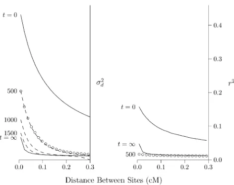
LD will decline following an expansion of population size, because genetic drift is weaker in large populations and produces less LD. This process is illustrated in Figure 2, which shows the effect of an expansion from size 2N= 103to 2N=
105. The LD curve of the initial population (labeledt= 0)
represents an equilibrium between mutation, drift, and re-combination. After the expansion, the LD curve will eventu-ally converge to a new equilibrium, which is labeledt=N. This new equilibrium, however, is reached only gradually.
LD is measured bys2
din Figure 2, left, and byr2in Figure
2, right. The dashed lines were calculated using the method of Hill (1975), and the open circles were estimated from data simulated using MACS (Chen et al. 2009). Note that s2
d is still far from equilibrium at generation 500 and does
not approach equilibrium until about generation 1500. The situation is very different in Figure 2, right, where LD is measured byr2. By generation 500,r2is close to
equilib-rium. At the left edge of the graph, it is slightly belowthe
Figure 2 Effect of population expansion on the LD curve. The population
grew suddenly at timet= 0 from 2N= 103 to 105. Left panel: LD is
measured bys2d:Solid lines show the predicted values at the initial
equi-librium (t= 0) and at the eventual equilibrium (t=N). Dashed lines show a series of transient states that occur at various values oft, the number of generations since the expansion. These lines are all calculated using the method of Hill (1975). Open circles show values simulated using MACS fort= 500. Right panel: LD is measured byr2, and points and lines are
based on computer simulation. Calculations assume thatu= 1.4831028
equilibrium. We return to this point later, but for the mo-ment, note simply thatr2converges much faster thans2
d:For
this reason, the two measures are useful for studying differ-ent timescales. We learn fromr2about the recent past and
froms2
dabout more ancient events. Presumably, this
differ-ence arises because s2
d is weighted toward loci with high
heterozygosity. As shown in Figure 1, this weighting makes it more sensitive to the distant past.
Returning to Figure 2, left, note that the right portion of the curve converges faster than the left. This is because the postexpansion population is large, and genetic drift is weak. The dynamics are therefore dominated by recombination, which is stronger on the right side of the graph. The result is that midway through the process—say at generation 500— the LD curve declines very steeply. Thus, a steeply declin-ing LD curve is the signature of recent population growth (Kruglyak 1999; Pritchard and Przeworski 2001).
The method of Hayes et al. (2003)
Figure 2 suggests thats2
dis likely to be of greater use thanr2
in inferring the ancient history of population size. Yet the latter statistic is often used instead (Hayeset al.2003; McEvoy
et al.2011; Tenesaet al.2007), using a method that is based on the formulaE[r2]r, where
r¼ 1
1þ4Nc: (4)
Here,Nis diploid population size, andcis the recombination rate (Sved 1971; Sved and Feldman 1973). Although this formula has been criticized (Littler 1973, p. 272; McVean 2002, pp. 987–988; McVean 2007, p. 923; Durrett 2008, p. 98), it is widely used.
Hayeset al.(2003) study a generalization ofr2and argue
from simulations that the expectation of this statistic isr. Furthermore, this approximation even works for populations that have increased in size at a constant linear rate, provided that one interpretsNas the population size that obtained 1/ 2cgenerations in the past. By inverting Equation 4, they are able to estimateNover a wide range of values of c, which correspond under their model to different points in the past. Tenesaet al.(2007) work directly withr2, but estimate
the history of population size in the same way. They also employ a modified predictor,
~ r¼ 1
2þ4Nc; (5)
which in their view accounts better for the effect of mutation. This method is also used by McEvoyet al.(2011). There are two difficulties with this formula. First, Tenesaet al.(2007, p. 521) derive it from a formula of Hill (1975, p. 124), which refers not toE[r2] but tos2
d:Thus, it approximatesE[r2] only
to the extent thats2
ddoes. In addition, it uses a fairly crude
standard of approximation, taking 10 as11.
The arguments justifying both of these methods assume that population size has increased linearly. Of course, no
population can increase linearly forever, so the period of linear increase must end at some point in the past. Further-more, the method’s results are often interpreted in terms of nonlinear growth trajectories, such as bottlenecks (Hayes
et al.2003, pp. 639–670; Tenesaet al.2007, p. 525; McEvoy
et al.2011, p. 822). Let us consider how the method behaves in this broader context.
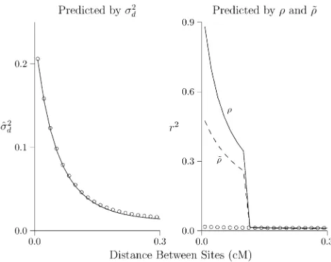
Figure 3 considers a population that expands suddenly in size and is observed 500 generations later. In both panels of Figure 3, the solid lines show predicted LD. In Figure 3, left, LD is measured bys^2dand predicted bys2d(Hill 1975). In Figure 3,
right, it is measured byr2and predicted byrand~r:The open
circles show values simulated using MACS (Chenet al.2009). In the context of this population history,s2
dprovides excellent
predictions ofs^2
d;but neitherrnor~rpredictsr2.
Presumably, this reflects the nonlinearity of the growth trajectory assumed in Figure 3. We expect better accuracy in Figure 4, which evaluatesrandr~against a history involving 300 generations of linear population growth, approximated as a series of 20 steps. The period of linear growth corresponds to the region to the right of the dashed line in Figure 4, right. At least in this region, predicted and simulated values should match. Yet as before,s2
dpredicts well, butrand~rdo not.
Finally, Figure 5 evaluatesr,~r;ands2
dagainst a history of
constant population size. In this case, we get an accurate prediction ofs^2dfroms2dand a fairly accurate prediction from
~
r:This makes sense, because (as mentioned above) ~ris an approximation to the equilibrium formula for s2
d: On the
other hand, neitherrnorr~provides a useful prediction ofr2.
In these analyses, the observed and predicted values ofr2
are distressingly far apart. Perhaps this discrepancy reflects an error in the simulation software (MACS) or in my own
Figure 3 Predicted and simulated LD. Each panel shows the same
pop-ulation 500 generations after expansion from 2N = 103 to 105. Lines
show values predicted bys2
d[left panel (Hill 1975)] and byr(right panel,
solid line) and ~r (right panel, dashed line). Open circles show results estimated from simulations. Calculations assume thatu= 1.4831028
code for estimating r2 from simulated data. To find out, I
used this software to replicate the published results of Hudson (1985). The results, shown in Figure 6, are reassuring. Given the same parameter values, the code used here produces results indistinguishable from those of Hudson.
It seems fair, therefore, to conclude that the problem lies in the predictors, rand~r;neither of which is useful in the cases studied here. It seems unlikely that they will be useful as a basis for inference in real populations.
Effect of population collapse
A collapse in population size produces an effect on the LD curve very different from that of population growth. This is shown in Figure 7, which illustrates two important points. First, the whole process is over very quickly. Even with s2
d;
we cannot look very far into the past. Second, the transient curves (the dashed lines) are quiteflat. As time passes, the initial curve (labeled t = 0) is elevated without much change in shape. Presumably, this is because the effect of drift is dominant in a small population, so differences in recombination rate do not matter much. The result is that the LD curve becomes high butflat after a collapse in pop-ulation size.
This pattern is superficially similar to that generated by gene conversion, which reduces LD between closely linked sites (Ardlie et al. 2001). It seems unlikely, however, that these effects will be confused. The effect of gene conversion is probably minor for sites separated by.1 kb (Frisseet al.
2001, p. 838; Chen et al. 2007, p. 764), whereas that of a population collapse extends much farther.
Effect of a bottleneck
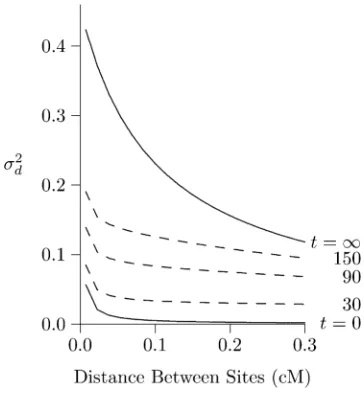
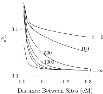
Figure 8 shows the effect of a 100-generation bottleneck in population size. Population size was 2N = 103during the
bottleneck but 105before and after. The bottleneck ended at
time 0, and we observe it in various subsequent generations. In the graph, the curve labeled t = 0 is at the end of the bottleneck and exhibits an LD curve that is high butflat, for reasons just discussed. As time passes, the right portion of
the curve (the portion with high rates of recombination) falls much faster than the left, so that by generation 1000, the curve is almost L shaped. This is the signature of a bot-tleneck in population size.
Note the dramatic difference between Figure 2 and Figure 8—between expansion from equilibrium and from a bottle-neck. Both curves are declining toward the same equilibrium, but the left portion of the curve declines much more slowly after a bottleneck than after expansion from equilibrium. This can only reflect the state of the population just before the increase in size. The initial population of Figure 2 had been small much longer than that of Figure 8. Consequently, it had less heterozygosity. As we see in the next section, this accel-erates the rate of decline in LD between closely linked sites. It is sometimes suggested that bottlenecks inflate long-range LD, just the opposite of the pattern seen above (Slatkin 2008, pp. 481–482; Tenaillonet al.2008). This discrepancy, however, evaporates on close inspection. When
Figure 4 Linkage disequilibrium (s^2
dorr2) after an
ep-isode of linear growth. The population begins at mutation-drift equilibrium with 2N= 103 and then
grows linearly to 2N = 106 over a period of 300
generations. Linear growth is approximated by 20 epochs of 15 generations, within each of which 2N is constant. In the right panel, the region to the right of the vertical line corresponds to the period of linear growth, according to the model of Hayes et al. (2003). All calculations assume that u = 1.48 3 1028andc = 1028 per nucleotide. Simulations
in-volve 109bp of DNA, which are sequenced in a
sam-ple of 100 homologous chromosomes.
Figure 5 LD curve under constant population size. Simulated values ofr2
ands^2
dwere generated using MACS (Chenet al.2009).s2dwas
calcu-lated using the method of Hill (1975),rwas calculated from Equation 4, and~rfrom Equation 5. All calculations assume that 2N= 1000,u= 1.483 1028, andc= 1028per nucleotide. Simulations involve 109bp of DNA,
Tenaillonet al.(2008,figure 6) discuss“long-range”LD, they are referring to pairs of nucleotide sites separated by0.01 cM. In my own analysis, such pairs would be called“tightly linked”and would fall at the left edge of the LD curve. In this region of Figure 8, LD is indeed elevated, in agreement with Tenaillon et al. (2008). In another study, Thornton and Andolfatto (2006, p. 1611) report elevated LD following a bottleneck. But as they do not discuss the shape of the curve, there is no conflict between their results and mine. The time paths of individual points on the LD curve
Figure 9 shows the time path of s2
d after an expansion in
population size. Because the new population is larger, the new equilibrium will have less LD. Buts2
ddoes not decline
monotonically toward this new equilibrium. Instead, it falls rapidly to a smaller value before climbing back slowly to-ward to the new equilibrium.
The initial decline ins2
ddoes not result from any decline
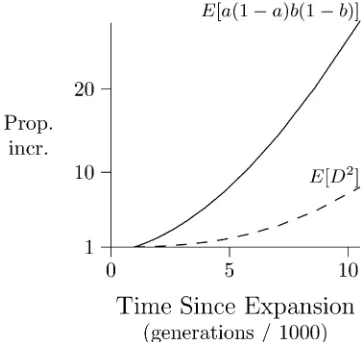
in its numerator, E[D2]. Indeed, Figure 10 shows that the
numerator actually grows. The decline in s2
d happens
be-cause growth in its numerator is outstripped by that in its denominator, E[a(12a)b(12 b)], which increases under the influence of mutation. The proportional increase is large, because our initial population was small and therefore had little heterozygosity. For this reason, the denominator was initially so small that increments caused by mutation had a large proportional effect.
Two factors account for the postexpansion growth in the numerator, E[D2], ofs2
d:First,D is proportional to
hetero-zygosity (Kaplan and Weir 1992, p. 334), which increases in response to mutation. Ordinarily, the positive effect on D2
would be offset by the negative effect of recombination. But in the early generations following our expansion, this nega-tive effect is very weak. This is because the initial population had low heterozygosity. Few recombinant gametes are duced in such a population, because such gametes are pro-duced only by double heterozygotes.
The nonmonotone time path in Figure 9 refers tos2 d;but
it seems plausible thatr2might obey similar dynamics. This
may explain why, in Figure 2, right, the left end of the curve fort= 500 is below the equilibrium.
This also explains why the left portion of the LD curve declines faster after expansion from equilibrium than after
a bottleneck. The left portion of the curve refers to tightly linked sites, with weak recombination. In the postexpansion population, genetic drift is also weak because the population is large. Because recombination and drift are both weak, mutation dominates the dynamics. The proportional effect of mutation is large when heterozygosity is low. In the case of expansion from equilibrium, the population has been small a long time, so heterozygosity is low, the proportional effect of mutation is large, and s2
ddeclines rapidly.
Hetero-zygosity is not so low at the end of a bottleneck, because the population has been small only briefly. Consequently, the proportional effect of mutation is smaller, and s2
d declines
more slowly.
LD in the human population of Europe
The methods discussed above generate predictions about LD from assumptions about the history of population size. It is also possible, by fitting predicted to observed curves, to work in the other direction—from data to inferences about
Figure 6 Replication of results of Hudson (1985, table 2). The left panel compares methods for calculating
s2
d; the right panel compares methods for calculating r2. The programs MACS, eld, and preld are described
inMaterials and Methods. Parameter values:u= 0.1, 2N= 50,000,n= 50. MACS simulated chromosomes 2 Mb in length. Following Hudson, I corrects^2
dbut not r2for sampling bias.
Figure 7 Effect of population collapse on the LD curve. At timet= 0, this population collapsed in size from 2N= 105to 103. Calculations use the
method of Hill (1975), withu= 1.4831028. No correction for sampling
population history. This is a problem in statistical inference, and methods for this purpose will be described elsewhere.
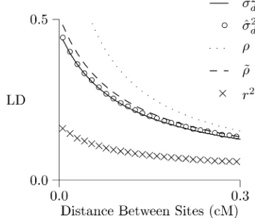
The present methods, however, are useful in exploratory data analysis, as shown in Figure 11. The open circles show ^
s2
d; as estimated from chromosome 1 in European data
(1000 Genomes Project Consortium 2012). These are sur-rounded by dashed lines, which indicate a 95% confidence region generated by moving-blocks bootstrap. These show that chromosome 1 provides accurate estimates ofs2
d:Hill
(1981) expressed skepticism about the possibility of estimat-ing population size from data on LD. At that time only lim-ited data were available, and it was not possible to estimate LD statistics with great accuracy. This inaccuracy bled into estimates of population size. The narrow confidence region in Figure 11 shows that things have changed.
The solid line in Figure 11 shows the equilibrium curve that
fits these data best—the one that minimizes squared errors between observed and predicted values ofs^2d:This is the curve
for a population of constant size, 2N= 8621. In Figure 11, right, we see the differences between observed andfitted val-ues. Because these differences are positive on the left but neg-ative on the right, it is clear that the observed LD curve declines more steeply than any equilibrium curve. As we have seen, this suggests a history of population expansion in Europe, in agree-ment with many other analyses of European data.
Discussion
s2
d has never been valued for its own sake. It is seen instead
as an approximation to the quantity of real interest—the expected value of r2. Yet it is often a poor approximation,
even in populations of constant size (Maruyama 1982; Hudson 1985, pp. 616–617). It is even worse when population size varies.
Following a change in population size, the mean of r2
converges toward its new equilibrium far faster than does s2
d:Presumably, this is because s 2
d is sensitive to loci with
high heterozygosity, and the gene trees of such loci are deep. Whatever the cause, this difference in rates of convergence has two effects. First, it makess2
duseless as an
approxima-tion to r2 in populations that have varied in size. On the
other hand, it also means that s2
ditself provides a deep
re-cord of demographic history.
To take advantage of this extended record, one must estimates2
ddirectly from data. This is easy to do, by using
averages in place of the expectations in Equation 2. With genome-scale data, such estimates are quite accurate. This provides a measure of LD that is unique in that one can easily calculate expected LD from the history of population size. With other measures, such inferences would require extensive computer simulations.
Following a population expansion, drift is weak and the dynamics of LD are dominated by recombination. The LD curve begins to decline, and this decline is fastest in the right-hand portion of the curve, where recombination rates are highest. Consequently, the curve will be unusually steep for hundreds of generations following a population expansion.
Following a population collapse, drift becomes strong and dominates the dynamics. It pushes LD upward rapidly
Figure 8 Effect of a 100-generation bottleneck in population size. The
curves shows2
dat various points after recovery from a 100-generation
bottleneck, during which the population had size 2N= 103. Before and
after the bottleneck, its size was 105. Other details are as in Figure 7.
Figure 9 The time path ofs2
dafter a population expansion. The initial
population was small (2N= 103) and at mutation–drift equilibrium. At
time 0 it expands suddenly to a much larger size (2N= 105). Each curve
shows the time path ofs2
dfor a different rate of recombination,
and relatively uniformly throughout the curve. Thus, the LD curve becomes high andflat. This pattern has been reported for several human populations, including high-latitude foragers (Kaessmannet al.2002) and Ashkenazi Jews (Shifman and Darvasi 2001). Yet as Pritchard and Przeworski (2001, p. 7) observe, it has been difficult to explain:
We have several examples in which large regions exhibit more LD than would be expected under either a model of constant population size or a model with rapid population growth. Yet, at the same time studies of polymorphism at a small scale reveal less LD than would be expected. These observations at different scales are hard to accommodate in a single explanation since factors that increase long-distance LD will tend to have an even larger effect on closely linked sites.
As we have seen, this pattern arises naturally from a recent reduction in population size.
A bottleneck in population size begins with an episode of population collapse. At the end of the bottleneck, the LD curve is therefore high butflat. As population size rises at the end of the bottleneck, genetic drift becomes weak and recombination grows in importance. The right portion of the LD curve falls faster than the left, so the curve becomes steeper.
In the left portion of the curve, recombination is weak. Genetic drift is also weak, because of the increase in pop-ulation size. This allows mutation to play an important role, and its effect distinguishes the two forms of expansion: from equilibrium and from a bottleneck. In the former case, the preexpansion population had little heterozygosity, so each mutational increment has a large proportional effect on the denominator ofs2
d:After a bottleneck, the opposite is true, so
the left portion of the LD curve declines more slowly. The curve becomes even steeper after a bottleneck than after an expansion from equilibrium.
In summary, (1) when recombination is strong relative to drift, LD declines and the curve becomes steeper; (2) when drift is strong relative to recombination, LD rises but the curve staysflat; and (3) where drift and recombination are both weak, the rate of decline in LD decreases with heterogyzosity.
In the human population of Europe, the LD curve is steep, suggesting a history of population expansion. This might reflect the spread of modern humans into Europe, the spread of farmers during the Neolithic, or the spread of Indo-European speakers.
Acknowledgments
I am grateful for comments from R. Bohlender, E. Cashdan, R. Gutenkunst, H. Harpending, W. G. Hill, and J. Seger and for access to computer facilities in the laboratories of Lynn Jorde and Henry Harpending.
Literature Cited
Ardlie, K., S. Liu-Cordero, M. Eberle, M. Daly, J. Barrett et al., 2001 Lower-than-expected linkage disequilibrium between tightly linked markers in humans suggests a role for gene con-version. Am. J. Hum. Genet. 69: 582–589.
Chen, G. K., P. Marjoram, and J. D. Wall, 2009 Fast andflexible simulation of DNA sequence data. Genome Res. 19: 136–142. Chen, J.-M., D. N. Cooper, N. Chuzhanova, C. Férec, and G. P.
Patrinos, 2007 Gene conversion: mechanisms, evolution and human disease. Nat. Rev. Genet. 8: 762–775.
Clark, A. G., M. J. Hubisz, C. D. Bustamante, S. H. Williamson, and R. Nielsen, 2005 Ascertainment bias in studies of human genome-wide polymorphism. Genome Res. 15: 1496–1502.
Figure 10 The time path of the numerator and denominator ofs2
d
fol-lowing a population expansion. Dashed line shows numerator of s2 d,
relative to its value in generation 1000. Solid line shows the denominator in the same way. Loci are separated by 0.02 cM. Population history is as in Figure 9.
Figure 11 LD curve for chromosome 1 in Europe. In the left panel, open
circles show the estimated values ofs2d;and dashed lines show a 95%
Dempster, A. P., N. M. Laird, and D. B. Rubin, 1977 Maximum likelihood from incomplete data via the EM algorithm. J. R. Stat. Soc. B 39: 1–38.
Durrett, R., 2008 Probability Models for DNA Sequence Evolution, Ed. 2. Springer-Verlag, New York.
Frisse, L., R. Hudson, A. Bartoszewicz, J. Wall, J. Donfacket al., 2001 Gene conversion and different population histories may explain the contrast between polymorphism and linkage dis-equilibrium levels. Am. J. Hum. Genet. 69: 831–843.
Fu, Y., 1995 Statistical properties of segregating sites. Theor. Popul. Biol. 48: 172–197.
Gao, F., and L. Han, 2012 Implementing the Nelder-Mead sim-plex algorithm with adaptive parameters. Comput. Optim. Appl. 51: 259–277.
Griffiths, R., and S. Tavaré, 1998 The age of a mutation in a gen-eral coalescent tree. Stoch. Models 14: 273–295.
Hamming, R. W., 1973 Numerical Methods for Scientists and En-gineers, Ed. 2. Dover, New York.
HapMap, 2007 A second generation human haplotype map of over 3.1 million SNPs. Nature 449: 851–862.
Hayes, B., P. Visscher, H. McPartlan, and M. Goddard, 2003 Novel multilocus measure of linkage disequilibrium to estimate past effective population size. Genome Res. 13: 635–643.
Hill, W. G., 1975 Linkage disequilibrium among multiple neutral alleles produced by mutation infinite population. Theor. Popul. Biol. 8: 117–126.
Hill, W. G., 1981 Estimation of effective population size from data on linkage disequilibrium. Genet. Res. 38: 209–216.
Hill, W. G., and A. Robertson, 1968 Linkage disequilibrium in finite populations. Theor. Appl. Genet. 38: 226–231.
Hudson, R. R., 1985 The sampling distribution of linkage disequi-librium under an infinite allele model without selection. Genet-ics 109: 611–631.
Kaessmann, H., S. Zöllner, A. C. Gustafsson, V. Wiebe, M. Laan et al., 2002 Extensive linkage disequilibrium in small human populations in Eurasia. Am. J. Hum. Genet. 70: 673–685. Kaplan, N., and B. Weir, 1992 Expected behavior of conditional
linkage disequilibrium. Am. J. Hum. Genet. 51: 333.
Kimura, M., 1969 The number of heterozygous nucleotide sites maintained in afinite population due to steadyflux of mutation. Genetics 61: 893–903.
Kruglyak, L., 1999 Prospects for whole-genome linkage disequi-librium mapping of common disease genes. Nat. Genet. 22: 139–144.
Lewontin, R. C., 1964 The interaction of selection and linkage. I. General considerations; heterotic models. Genetics 49: 49–67. Lewontin, R. C., 1967 An estimate of average heterozygosity in
man. Am. J. Hum. Genet. 19: 681–685.
Lieu, R. Y., and K. Singh, 1992 Moving blocks jacknife and boot-strap capture weak dependence, pp. 225–248 inExploring the “Limits”of the Bootstrap, edited by R. LePage, and L. Billard. John Wiley & Sons, New York.
Littler, R., 1973 Linkage disequilibrium in two-locus,finite, ran-dom mating models without selection or mutation. Theor. Popul. Biol. 4: 259–275.
Maruyama, T., 1982 Stochastic integrals and their application to population genetics, pp. 151–166 inMolecular Evolution,Protein Polymorphism, and the Neutral Theory, edited by M. Kimura. Springer-Verlag, Berlin.
McEvoy, B., J. Powell, M. Goddard, and P. Visscher, 2011 Human population dispersal“out of Africa”estimated from linkage disequi-librium and allele frequencies of SNPs. Genome Res. 21: 821–829.
McVean, G., 2002 A genealogical interpretation of linkage dis-equilibrium. Genetics 162: 987–991.
McVean, G., 2007 Linkage disequilibrium, recombination and se-lection, pp. 909–944 inHandbook of Statistical Genetics, Ed. 3, edited by D. Balding, M. Bishop, and C. Cannings. John Wiley and Sons, Chichester, UK.
Ohta, T., and M. Kimura, 1969 Linkage disequilibrium at steady state determined by random genetic drift and recurrent muta-tion. Genetics 63: 229.
Ohta, T., and M. Kimura, 1971 Linkage disequilibrium between two segregating nucleotide sites under the steadyflux of muta-tions in afinite population. Genetics 68: 571–580.
1000 Genomes Project Consortium, 2012 An integrated map of genetic variation from 1,092 human genomes. Nature 491: 56– 65.
Press, W. H., S. A. Teukolsky, W. T. Vetterling, and B. P. Flannery, 1992 Numerical Recipes in C: The Art of Scientific Computing, Ed. 2. Cambridge University Press, New York.
Pritchard, J., and M. Przeworski, 2001 Linkage disequilibrium in humans: models and data. Am. J. Hum. Genet. 69: 1–14. Rogers, A. R., and C. Huff, 2009 Linkage disequilibrium between
loci of unknown phase. Genetics 182: 839–844.
Rogers, A. R., and L. B. Jorde, 1996 Ascertainment bias in esti-mates of average heterozygosity. Am. J. Hum. Genet. 58: 1033– 1041.
Schaper, E., A. Eriksson, M. Rafajlovic, S. Sagitov, and B. Mehlig, 2012 Linkage disequilibrium under recurrent bottlenecks. Ge-netics 190: 217–229.
Shifman, S., and A. Darvasi, 2001 The value of isolated popula-tions. Nat. Genet. 28: 309–310.
Slatkin, M., 2008 Linkage disequilibrium—understanding the evolutionary past and mapping the medical future. Nat. Rev. Genet. 9: 477–485.
Song, Y., and J. Song, 2007 Analytic computation of the expecta-tion of the linkage disequilibrium coefficientr2. Theor. Popul.
Biol. 71: 49–60.
Strobeck, C., and K. Morgan, 1978 The effect of intragenic re-combination on the number of alleles in a finite population. Genetics 88: 829–844.
Sved, J. A., 1971 Linkage disequilibrium and homozygosity of chromosome segments infinite populations. Theor. Popul. Biol. 2: 125–141.
Sved, J. A., 2009 Correlation measures for linkage disequilibrium within and between populations. Genet. Res. 91: 183–192. Sved, J. A., and M. W. Feldman, 1973 Correlation and probability
methods for one and two loci. Theor. Popul. Biol. 4: 129–132. Tenaillon, M., F. Austerlitz, and O. Tenaillon, 2008 Apparent
mu-tational hotspots and long distance linkage disequilibrium re-sulting from a bottleneck. J. Evol. Biol. 21: 541–550.
Tenesa, A., P. Navarro, B. Hayes, D. Duffy, G. Clarke et al., 2007 Recent human effective population size estimated from linkage disequilibrium. Genome Res. 17: 520–526.
Thornton, K., and P. Andolfatto, 2006 Approximate Bayesian in-ference reveals evidence for a recent, severe bottleneck in a Netherlands population ofDrosophila melanogaster. Genetics 172: 1607–1619.
Weir, B., and C. Cockerham, 1974 Behavior of pairs of loci infinite monoecious populations. Theor. Popul. Biol. 6: 323–354. Weir, B. S., 1996 Genetic Data Analysis II: Methods for Discrete
Population Genetic Data. Sinauer Associates, Sunderland, MA.
Appendix
Hill’s model of LD evolution
Hill (1975) incorporates mutation, using the model of infinite alleles. However, most modern work involves either DNA sequence data or SNPs. In these data, alleles are nucleotide states: A, T, G, or C. Nearly all loci have just two alleles, so it is not appropriate to assume an infinity of alleles. Yet as we shall see, Hill’s (1975) results also apply to a more appropriate mutational model—that of“infinite sites”(Kimura 1969), which assumes that mutation never strikes the same site twice.
Hill begins with a vector of moments:
yhi;jk¼
0 B B @
Eahaibjbk
EahbjDikþahbkDij
þ aibjDhkþaibkDhj
EDhjDikþDhkDij
1 C C A:
Hereaiand bjare the frequencies of alleleAiat locus Aand allele Bjat locus B. The disequilibrium coefficients,Dij, are
defined such thataibj+Dijis the frequency of gamete typeAiBj. The dynamics of these moments are approximately linear,
after dropping terms inu2, 1/N2, andu/N, whereuis the mutation rate andNthe diploid population size. Thus, Hill (1975,
equation 1) shows that
yhi;jkðtþ1Þ DRMyhi;jkðtÞ;
where D, R, and M are matrices describing the linear effects of drift, recombination, and mutation. So far, the model describes only the changes in frequency of existing alleles. Thus it applies not only to Hill’s model of infinite alleles, but also to the model of infinite sites.
To incorporate mutation, Hill defines a new vector,
x¼X
h6¼i
X
j6¼k
yhi;jk; (A1)
where the sums run across all pairs of alleles at each locus. The dynamics of this new vector include an additive contribution,
Dxmut, which represents the effect of mutation to new alleles:
xðtþ1Þ DRMxðtÞ þDxmutðtÞ: (A2)
This equation can be iterated across many generations, and it is easy to incorporate changes in population size. At the end of this process,s2
dis calculated asx3/2x1(Hill 1975, p. 124).
The first term on the right side of Equation A1 applies equally to both mutational models. Some reinterpretation is required, however, to relate the second term to the model of infinite sites. In this new context,Dxmutbecomes the contri-bution of mutations at other sites in the genome, rather than that from new alleles at the same pair of sites. The mutational increments are, however, identical in the two models.
To see that this is so, let us take a close look at the mutational contributions tox, the vector defined above in Equation A1. Under the model of infinite sites, mutation never strikes the same site twice, so each polymorphic site has exactly two alleles. In this biallelic context, we can simplify Hill’s vector of moments as
h¼ 0
@EE½ð1½að1222aaÞð1Þbð1222bbÞÞD ED2
1
A: (A3)
Here,aandbare the frequencies of allelesA1andB1, andDis the coefficient of linkage disequilibrium. It is defined such that
ab +Dis the frequency of gamete typeA1B1. When each locus is biallelic, Hill’s multiallelic moments reduce tox1= 4h1,
x2= 4h2, andx3= 8h3(Hill 1975, p. 123).
The mutational increments, DxmutandDhmut, both depend on the heterozygosity,H=E[2a(12a)]. The dynamics of heterozygosity under infinite sites are the same as those under infinite alleles (Hill 1975, p. 120):
Htþ12uþ
12 1
2N22u
The hiare nonzero only if both loci are polymorphic. On the other hand, our model assumes that mutation affects only
monomorphic sites. This implies that mutational increments tohoccur only at pairs of sites in which one site is polymorphic and the other monomorphic. Table A1 summarizes the case in whichAis initially polymorphic, and a mutation strikes an initially monomorphic locus,B.
Considerfirst the increment toh1=E[a(12a)b(12b)]. Before mutation,h1= 0 becauseb= 0. After mutation,b= 1/2N, soh1becomesE[a(12a)(1/2N21/4N2)]H/4N. This accounts for only half the effect of mutation, because there
are also pairs at which Ais monomorphic and B polymorphic. The expected effect of a single mutation is thus H/2N. The expected number of such mutations per generation is 2Nu. In aggregate, therefore, the increment from mutation is
Dmuth1uH.
To derive the mutational increment toh2=E[(122a)(122b)D], we assume as before thatAis polymorphic butBis not. BecauseDis zero when either site is monomorphic,h2= 0 before mutation. After mutation, there are two cases to consider. With probabilitya, the mutation falls on anA1-bearing gamete, andh2becomes (122a)(122/2N)(12a)/2N, as shown in Table A1. On the other hand, with probability 12athe mutation falls on anA0-bearing gamete, andh2becomes2(122a) (122/2N)a/2N. In expectation, the new value ofh2is 0. This result is conditional on a mutation at locusB, but an identical argument applies for mutation at locusA. Thus,Dmuth2= 0.
The third moment ish3=E[D2]. BecauseBis initially monomorphic,D2= 0 before the mutation. When a mutation occurs
atB, it strikes anA1-bearing gamete with probabilityaand anA0-bearing gamete with probability 12a. The resulting values ofDare shown in Table A1. Squaring these and weighting byaand 12a gives
E "
a (
ð12aÞ2
4N2
)
þ ð12aÞ
a2
4N2
¼ H
8N2:
This is the effect onD2of a single mutation atB. There are 2Nusuch mutations per generation, so the expected increment
from mutation at locus B is 2Nu 3H/8N2 =uH/4N. Finally, multiply by 2 to account for cases in which Ais initially
monomorphic andBpolymorphic. This givesDmuth3=uH/2N0, ignoring terms of orderu/N. In summary,
Dmuth ½uH;0;0; (A4)
in agreement with Hill (1975, p. 121). This shows that the mutational increment is the same under the models of infinite sites and infinite alleles. Because of this equivalence, Hill’s results apply equally to both models of mutation.
Estimating Linkage Disequilibrium with Partially Phased Diploid Data
In 1000-genotypes data, not all genotypes are phased. At different loci, the unphased genotypes may correspond to different individuals. Thus, we need a method that can deal with unphased genotypes scattered throughout the data matrix.
The symbolsj,k,l, andmrepresent alleles and will always equal either 0 or 1. I write phased two-locus genotypes in form
jk
lm;which says that a diploid individual has genotypejkat locusAand genotypelmat locusB. This represents the union of
gametes j
l and k
m:This genotype is unordered, in that we cannot distinguish the maternal gamete from the paternal one.
Consequently, there is no distinction between jk
lm and kj
ml:When I write genotypes in this form, I imply that linkage phase is
known. In other words, genotypes jk
lm and jk
ml are not equivalent.
Consider a tiny two-locus data set, consisting of three diploid individuals:
Table A1 Effect of a single mutation atB, assuming thatAis initially polymorphic
Gamete frequencies
Case A1B1 A1B0 A0B1 A0B0 D
General w x y z wz2xy
Before mutation 0 a 0 12a 0
A1-linked mutation 1/2N a21/2N 0 12a (12a)/2N
G1;G1;G3¼ j1k1
l1m1;
j2k2
l2m2;
j3k3
l3m3:
On the right, each row corresponds to a locus and each column to a gamete. To estimate linkage disequilibrium (D), we would need to calculateS¼P6i¼1xiyi;wherexiis theith value in the upper row andyiis the corresponding value in the
lower one. This sum can be written as
S¼s1þs2þs3¼ ðj1l1þk1m1Þ þ ðj2l2þk2m2Þ þ ðj3l3þk3m3Þ:
Here,si=jili+kimiis the contribution of theith diploid genotype. This calculation requires phased data, and it is the only
step where such data are required in estimating D. To cope with unphased data, we need a method to estimatesi.
Consider the function s
jk lm
¼jlþkm:If at least one genotype is homozygous, then phasing does not matter. For
example, s
jk ll
¼s
kj ll :
We can calculate sregardless of phasing. The only genotypes that need concern us are those in which both loci are heterozygous.
As mentioned above, all genic values (j,k,l, andm) are either 0 or 1. Double heterozygotes will look like either01 01 or
01 10: (I ignore the equivalent representations 10
10 and 10
01;because genotypes are unordered.) With unphased data, we cannot distinguish between these two cases. Yet they imply different values:s
01 01
¼1 buts
01 10
¼0:For double heterozygotes,
I replace swith its expected value, which equals the probability,w, that the genotype is of form 01
01 rather than 01 10: To calculate this probability, I begin with standard results for the frequencies of the four gamete types, as shown in Table A2. Following Rogers and Huff (2009), I ignore recombination in the most recent generation. Under random mating, these gametes form at random to produce two-locus genotypes. The frequency of genotype 01
01 among double heterozygotes is thus
w¼ 2p0p3
2p0p3þ2p1p2
¼ DþZ
Dþ2Z;
(A5)
where
Z¼a2bDþD2;
a¼að12aÞbð12bÞ;
and
b¼aþb22ab:
These results can be used to estimate D using the EM algorithm (Dempster et al. 1977). LetKrepresent the number of unphased double heterozygotes. Each of these is of type 01
01 with probabilitywand of type 01
10 with probability 12w. The expected log likelihood is
ElnL¼X
3
i¼0
nilnpiþK½wðlnp0þlnp3Þ þ ð12wÞðlnp1þlnp2Þ
¼ ðn0þKwÞlnp0þ ðn1þKð12wÞÞlnp1þ ðn2þKð12wÞÞlnp2þ ðn3þKwÞlnp3:
Note thatElnLdepends onp0,p1,p2, andp3, which are themselves functions ofD. The maximum-likelihood estimate ofDis the value that maximizesElnL.
This is a unidimensional maximization problem, becauseDis the only unknown.Dcannot fall outside the range½D;D;
(Hamming 1973, p. 68). If the result is within½D;D;then the Newton step is accepted. Otherwise, the algorithm uses a modified version of the bisect algorithm (Hamming 1973, p. 62) to move in the uphill direction, as indicated by the sign ofdElnL/dD. The modification to bisect allows the algorithm to make large steps when it seems likely that the optimum is at a boundary. For example, ifdElnL/dD.0 at the current value ofD, then motion is to the right, towardD:Before deciding how far to move, the algorithm checks the sign of the derivative atD:If both derivatives are positive, then the algorithm takes a big step, moving 80% of the distance fromDtoD:But if the two derivatives have opposite sign, then the algorithm takes a small step, moving only 50% of the way toD:WhendElnL/dD,0, the algorithm is similar, except that motion is to the left, towardD:
Table A2 Gamete types and frequencies
Gamete Sample count Population frequency
0 0
n0 p0= (12a)(12b) +D
0 1
n1 p1= (12a)b2D
1 0
n2 p2=a(12b)2D
1 1
n3 P3=ab+D
niis the number of copies of gameteiin the sample, excluding unphased double heterozygotes.piis the frequency of that gamete type within the