Gradient-Free Active Subspace Construction and Model Calibration Techniques for Complex Models.

ABSTRACT

LEWIS, ALLISON LEIGH. Gradient-Free Active Subspace Construction and Model Calibration Techniques for Complex Models. (Under the direction of Dr. Ralph C. Smith.)

As physical models used in large-scale applications become increasingly complex and computa-tionally demanding, numerous issues related to the field of uncertainty quantification (UQ) must be addressed. Knowledge of topics such as model calibration, parameter selection, uncertainty propa-gation, and surrogate modeling have become essential to researchers in a wide array of fields. In this dissertation, we focus on two aspects of UQ: (i) model calibration in a high-to-low fidelity framework, and (ii) gradient-free construction of active subspaces for emulation via response surfaces.

We first develop an information-theoretic approach to calibrating low-fidelity codes using simulated data from validated high-fidelity models, which are prohibitively expensive to evaluate repeatedly. Our objective is to employ a minimal number of high-fidelity code evaluations as syn-thetic data for Bayesian calibration of the low-fidelity code under consideration. We employ the mutual information between low-fidelity model parameters and experimental designs to determine input values to the high-fidelity code, which maximize the available information. For computa-tionally expensive codes, surrogate models may be used to approximate the mutual information. We illustrate this framework using a comprehensive set of numerical examples, including several relevant to nuclear power plant design.

Gradient-Free Active Subspace Construction and Model Calibration Techniques for Complex Models

by

Allison Leigh Lewis

A dissertation submitted to the Graduate Faculty of North Carolina State University

in partial fulfillment of the requirements for the Degree of

Doctor of Philosophy

Applied Mathematics

Raleigh, North Carolina 2016

APPROVED BY:

Dr. H. Thomas Banks Dr. Mansoor A. Haider

Dr. Brian J. Reich Dr. Ralph C. Smith

DEDICATION

BIOGRAPHY

Allison was born in Schenectady, NY and spent her elementary through high school years in Ken-newick, WA and Lynchburg, VA. During that time she discovered an affinity for math and science, and decided to attend the University of Portland, majoring in mathematics. While in college, she participated in a mathematics research program at Williams College, which solidified her desire to continue with graduate studies.

After graduating Magna cum Laude from the University of Portland, she attended North Carolina State University, completing her Master’s degree in Applied Mathematics in 2013 and defending her Ph.D. thesis in May 2016. In the spring of 2016, she accepted a position in the Air and Missile Defense sector at The Johns Hopkins University Applied Physics Laboratory.

ACKNOWLEDGEMENTS

First of all, I would like to extend a huge thank you to my advisor, Dr. Ralph Smith. I was honored to be approached by you three years ago, and I appreciate everything you have done for me since. I’ve learned so much these past few years besides just math. I’ve learned that research is NOT easy, and that sometimes no matter how hard you work, you don’t get the results you want or expect. After all, “we don’t make the news, we just report it." But I’ve also learned that no matter how difficult, the end result is absolutely worth it. I am so proud of the work I have done with you the past three years; I never thought I was capable of this. I would also like to thank my other committee members, Dr. Haider, Dr. Banks, and Dr. Reich, for their time and valuable feedback during this process.

There are a number of people who have contributed to the work in this dissertation in the form of stimulating discussions and generation of ideas, as well as co-authorship of papers. These include, but are not limited to, Brian Williams (LANL), Victor Figueroa, Vincent Mousseau, and Brian Adams (Sandia), Max Morris (ISU), Paul Constantine (CSM), Gabriel Terejanu (USC), and Bassam Khuwaileh and Katie Schmidt (NCSU).

And speaking of Katie, I would like to thank you for keeping me sane these past few years! We’ve had a lot of laughs and a more than a few meltdowns, and I’m fairly sure I wouldn’t have made it to the finish line without our "buddy system". I’m proud of us.

I owe my early success in mathematics and the fact that I even made it as far as graduate school to a whole host of wonderful teachers over the years. From the 7th grade, where I first discovered a love for math in my honors algebra class, to the incredible support I had from the entire math department at the University of Portland, to my wonderful research advisor at Williams College, Dr. Steven Miller, I was never lacking in encouragement. You all made me believe in myself.

And last but not least, I want to thank my family for all of their support and encouragement over the years. My wonderful parents, Chris and Joann Lewis, are true role models for parenting. They raised me to believe that I could accomplish whatever I dreamed of, and they backed those dreams 100%. My two incredible sisters, Michelle and Kellie, continue to inspire me on a daily basis and push me to better myself. I love you all. This dream come true was truly a team effort, and I share my success with all of you.

TABLE OF CONTENTS

LIST OF TABLES . . . vii

LIST OF FIGURES. . . .viii

I Introductory Material 1 Chapter 1 Overview of Topics . . . 2

1.1 High-to-Low Fidelity Model Calibration . . . 4

1.2 Gradient-Free Active Subspace Methods . . . 6

Chapter 2 Applications . . . 10

2.1 Neutron Transport . . . 10

2.1.1 SCALE6.1 . . . 13

2.2 Thermal-Hydraulics . . . 15

2.2.1 Hydra-TH . . . 16

2.2.2 COBRA-TF . . . 19

II High-to-Low Fidelity Model Calibration 21 Chapter 3 High-to-Low Framework. . . 22

3.1 Design Framework . . . 22

3.2 kNN Estimate of Mutual Information . . . 25

3.2.1 ANN Search Algorithm . . . 28

3.3 Verification of Mutual Information Algorithms . . . 29

3.3.1 Monte Carlo Method . . . 29

3.3.2 Verification Example . . . 30

3.4 Numerical Examples . . . 31

3.4.1 Steady State Heat Model . . . 32

3.4.2 Time-Dependent Diffusion Model . . . 36

3.4.3 Neutron Diffusion Model . . . 37

3.4.4 Particle Transport Model . . . 41

3.4.5 Hydra-TH CFD Code: Poiseuille Flow in a Pipe . . . 45

III Gradient-Free Methods for Active Subspace Construction 50 Chapter 4 Active Subspace Construction. . . 51

4.1 Methods for Construction . . . 52

4.1.1 Gradient-Based Active Subspace Method . . . 54

4.1.2 Gradient-Free Active Subspace Methods . . . 54

4.2.1 Gap-Based Dimension Selection . . . 61

4.2.2 Error-Based Dimension Selection . . . 62

4.2.3 PCA Dimension Selection . . . 63

4.2.4 Response Surface Dimension Selection . . . 64

4.3 Initialization Algorithm . . . 65

Chapter 5 Proof of Convergence . . . 69

5.1 Finite Sampling Convergence . . . 70

5.2 Approximate Gradient Convergence . . . 75

5.3 Adaptive Morris Convergence . . . 79

Chapter 6 Numerical Examples. . . 82

6.1 Elliptic PDE . . . 82

6.1.1 β=1: Rapid Eigenvalue Decay . . . 84

6.1.2 β=0.01: Gradual Eigenvalue Decay . . . 87

6.2 Extended Elliptic PDE . . . 90

6.3 SCALE6.1 Examples . . . 92

6.3.1 44-Dimensional Input Space . . . 93

6.3.2 132-Dimensional Input Space . . . 96

6.3.3 7700-Dimensional Input Space . . . 98

Chapter 7 Conclusions . . . .102

REFERENCES . . . .105

APPENDICES . . . .111

Appendix A Delayed Rejection Adaptive Metropolis Algorithm . . . 112

LIST OF TABLES

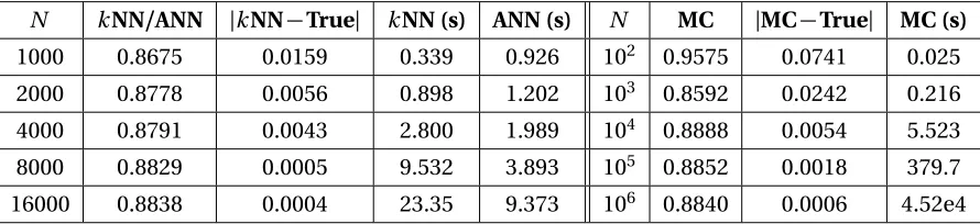
Table 2.1 Thermal-hydraulics parameters for the mass, momentum, and energy conserva-tion equaconserva-tions. . . 16 Table 3.1 Mutual information values forkNN, ANN, and Monte Carlo algorithms with

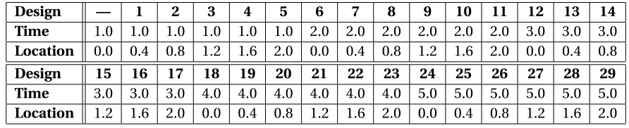
varying numbers of samples to verify the convergence to the analytic value. Running times are reported in seconds for each method. . . 31 Table 3.2 Possible design choices for the steady state heat equation example. . . 33 Table 3.3 Design choice sequence for the Monte Carlo,kNN, and ANN algorithms in the

steady state heat equation example. . . 34 Table 3.4 L2errors for the steady state heat equation at each of the 12 design selection steps. 36 Table 3.5 Possible design choices for the time-dependent heat equation example. . . 37 Table 3.6 Comparison of design sequences provided by the Monte Carlo,kNN, and ANN

methods for the time-dependent heat equation example. . . 37 Table 3.7 Possible design conditions for the neutronics example. . . 40 Table 3.8 Estimated mutual information values and sequential design sequence for the

neutronics example from Algorithms 1 and 2. . . 40 Table 3.9 Comparison of pressure gradients, velocities, and friction factors provided by

the Hydra-TH CFD code as compared to the analytic values from (2.17), (3.22), and (3.22). . . 46 Table 3.10 Estimated mutual information values computed via thekNN algorithm and

sequential design sequence for the Hydra-TH high-to-low computation. . . 48 Table 6.1 Active subspace dimension selections for gap-based criteria[11], principal

com-ponent analysis with varying threshold values[22], and error-based criteria with varying tolerances[18]for the 44-input example. . . 95 Table 6.2 Active subspace dimension selections for gap-based criteria[11], principal

com-ponent analysis with varying threshold values[22], and error-based criteria with varying tolerances[18]for the 132-input example. . . 97 Table 6.3 Reaction types and descriptions for the 7700-input example[19, 46]. . . 98 Table 6.4 Active subspace dimension selections for gap-based criteria[11], principal

LIST OF FIGURES

Figure 1.1 Schematic of topics in uncertainty quantification[53]. . . 3 Figure 2.1 (a) Pressurized water reactor (PWR) schematic. Image courtesy of United States

Nuclear Regulatory Commission. (b) Nuclear fuel assembly. . . 11 Figure 2.2 Configuration of laminar pipe flow. . . 18 Figure 2.3 (a) Laminar flow schematic. (b) Hexahedron mesh for describing laminar flow

in a pipe. . . 19 Figure 3.1 Calculation ofε(i),n_θ(i), andnd(i)for the casek=1 from[30]. Here we have

n_θ(i) =3 andnd(i) =4. Note that thekth-nearest neighbor is not included in the determination ofn_θ andn_d. . . 26 Figure 3.2 High-fidelity parameter distributions used to construct “experimental data”. . . 33 Figure 3.3 (a) Well-mixed parameter chains from DRAM, and (b) Joint posterior

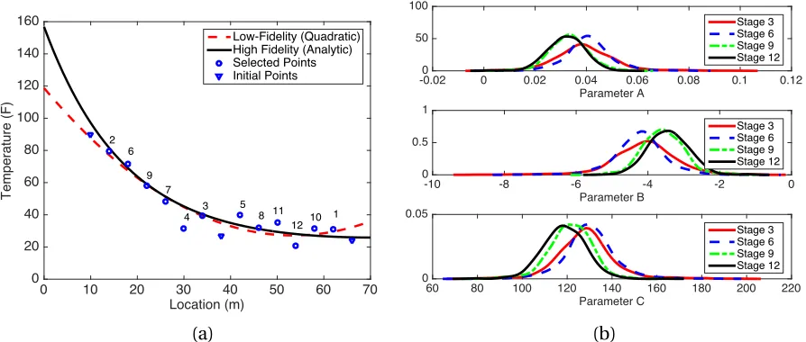
distribu-tions for pairwise combinadistribu-tions ofθ= [A,B,C]. . . 34 Figure 3.4 (a) Fit of quadratic model to the steady state heat equation analytic solution

for 15 total calibration points, with ordering selected by thekNN algorithm. (b) Evolution of parameter distributions for the steady state heat equation over 12 cycles of the design algorithm. . . 35 Figure 3.5 High-fidelity solution versus calibrated low-fidelity time-dependent heat

mod-els in (a) time domain[0, 5]for eleven uniformly spaced values ofx on the interval[0, 2], (b) spatial domain[0, 2]for eleven uniformly spaced values oft on the interval[0, 5], and (c) 3-dimensional domain. (d) Difference between the low- and high-fidelity solutions. . . 38 Figure 3.6 (a) High-fidelity versus low-fidelity models and (b) evolution of parameter

dis-tributions for the neutronics example. . . 41 Figure 3.7 Well-mixed parameter chains for the particle transport example. . . 43 Figure 3.8 (a) Marginal parameter densities for the particle transport model, calculated

from the final 3,000 iterations in a 10,000 iteration DRAM run, and (b) joint posterior distribution for the parameter setθ= [D,Σa]. . . 44 Figure 3.9 High-fidelity simulated experimental data versus low-fidelity measurements

for the particle transport model. Note the widening of the 95% credible interval (indicated in dark gray) and the 95% prediction interval (indicated in light gray) as the distance between measurements increases. . . 44 Figure 3.10 Configuration of laminar pipe flow. . . 45 Figure 3.11 Comparison of calibrated low-fidelity exponential model versus the high-fidelity

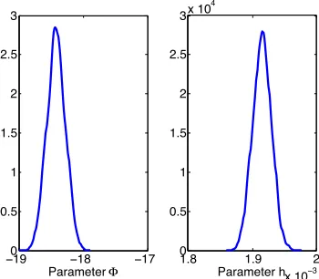
Hydra-TH code. Analytic values provided by (3.22) are shown to demonstrate bias present in high-fidelity model. . . 47 Figure 3.12 Hydra-TH parameter distributions for nine iterations of the mutual information

design algorithm. . . 49 Figure 4.1 Contour map depicting function variability over the input space for the function

Figure 4.2 Examples of steps on a two-dimensional input grid with a random initial point x∗_{. One elementary effect is computed per direction, for a total ofm+1 function} evaluations. (a) Finite-difference Morris steps where step sizes are constant and step directions are aligned with the input space. (b) Adaptive Morris steps where steps are taken in the primary directions of the active subspace with step sizes determined by the significance of the corresponding eigenvalues. . . 58 Figure 4.3 (a) First iteration of Algorithm 8. Pointsxandyare chosen on the unit m-sphere

centered atx0_{. The maximum function evaluation over the great circle defined}

byxandyoccurs at the pointz+. (b) Second iteration of Algorithm 8. The pointx has been updated to the valuez+from the previous iteration. A newyis chosen, and the function is optimized over the new great circle. . . 66 Figure 6.1 (a) Normalized eigenvalues of the gradient matrixGor gradient estimate ˜Gfor

three active subspace methods forβ=1. (b) First 30 components of the first eigenvector for each active subspace method. . . 85 Figure 6.2 (a) Final column of rotated elementary effects from the adaptive Morris method.

Note that the greatest variability is measured in the first direction, with elemen-tary effects quickly leveling off to zero. (b) Closeup of first 20 rotated elemenelemen-tary effects. . . 86 Figure 6.3 One-dimensional kriging surface projections for (a) the local sensitivity method,

(b) gradient-based method, (c) finite-difference Morris method, and (d) adaptive Morris method for β =1. Five training points are used to train the kriging surfaces and mean kriging predictions are plotted with a solid line. We plot 300 testing evaluations to depict how closely the function on the kriging surface matches the behavior of the function on the original surface. . . 86 Figure 6.4 Comparison of 300 testing point function evaluations on the original full surface

versus the constructed one-dimensional kriging surface forβ=1. Data for each of the three active subspace methods is plotted along with the results of the local sensitivity method: (a) gradient-based, (b) finite-difference Morris, and (c) adaptive Morris. . . 87 Figure 6.5 (a) Singular values of the gradient matrixGor gradient estimate ˜Gfor three

active subspace methods forβ=0.01. (b) First, and (c) second eigenvectors for each of the active subspace methods. . . 88 Figure 6.6 One-dimensional kriging surface projections for the (a) local sensitivity method,

Figure 6.7 Two-dimensional kriging surface projections for (a) the local sensitivity method, (b) gradient-based method, (c) finite-difference Morris method, and (d) adaptive Morris method forβ=0.01. Five training points are used to train the kriging surfaces and mean kriging predictions are plotted with a solid plane. We plot 300 testing evaluations to depict how closely the function on the kriging surface matches the behavior of the function on the original surface. . . 89 Figure 6.8 Comparison of 300 testing point function evaluations on the original full

sur-face versus the constructed kriging sursur-face forβ=0.01. Data for each of the three active subspace methods is plotted alongside the results of the sensitivity method. One-dimensional kriging surfaces are plotted for (a) gradient-based, (b) finite-difference Morris, and (c) adaptive Morris. Two-dimensional kriging surfaces are plotted for (d) gradient-based, (e) finite-difference Morris, and (f ) adaptive Morris. . . 90 Figure 6.9 (a) Singular values of the gradient matrix or approximation for each of the three

active subspace methods. We note the gap in magnitude between eigenvalues 10 and 11 for each method. (b) Relative errors|f −fs|/|f|at testing points outside of the active subspace for response surfaces constructed with piecewise linear interpolation over an active subspace of dimension 10. (b) Maximum, mean, and minimum relative errors|f −fs|/|f|at 10,000 testing points outside of the active subspace for response surfaces constructed via piecewise linear interpolation over active subspaces of dimensionsk =1, ..., 14. . . 92 Figure 6.10 (a) PWR pin cell construction for the 44-input neutron transport example. (b)

Material composition of the PWR quarter fuel lattice for the 132- and 7700-input neutron transport examples. . . 93 Figure 6.11 (a) Singular values for the 44-input example for each of the three active subspace

methods. (b) Error upper bounds given by Algorithm 5 for the 44-input example. 94 Figure 6.12 Comparison ofk_effresponses at testing points and constructed response surface

for a one-dimensional active subsapce for the (a) gradient-based, (b) finite-difference Morris, and (c) adaptive Morris methods for the 44-input example. . . 95 Figure 6.13 (a) Eigenvalues for the 132-input example. (b) Error upper bounds given by

Algorithm 5 for the 132-input example. . . 96 Figure 6.14 Comparison ofkeffresponses at testing points and constructed response surface

for one-dimensional active subspaces for the (a) gradient-based, (b) adaptive Morris, and (c) initialized adaptive Morris methods, and two-dimensional active subspaces for the (d) gradient-based, (e) adaptive Morris, and (f ) initialized adaptive Morris methods for the 132-input example. . . 97 Figure 6.15 (a) First 300 eigenvalues for the 7700-input example. (b) Response surface RMSE

values for the first 450 dimensions. (c) First 350 error upper bounds given by Algorithm 5 for the 7700-input example. . . 99 Figure 6.16 Observed versus predictedkeff values for (a) 25, (b) 75, (c) 150, and (d) 300

Part I

CHAPTER

1

OVERVIEW OF TOPICS

Uncertainty quantification is rapidly growing as a result of increasingly complex physical mod-els and scientists’ and engineers’ recognition of the need for a framework that can facilitate the prediction of future outputs with quantified uncertainties. Sources of error in these models may include approximation errors, uncertainties in the inputs or parameters, errors in experimental data acquisition, and errors resulting from numerical methods. One goal of uncertainty quantification is to predict how these errors and uncertainties will propagate through the models and design prediction intervals for relevant quantities of interest.

The process of uncertainty quantification can be broken down into two main steps. The first revolves around the calibration of the model to fit physical data that may be available experimentally or from another validated code. Given expected output values in the form of physical data, we can infer the parameter distributions that would lead the model to produce these outputs. In a Bayesian framework, which we use throughout this investigation, we consider inputs to be random variables with associated densities, rather than treating them as fixed but unknown values as we would in a frequentist perspective. The Bayesian framework is natural to employ for uncertainty quantification, since the use of parameter densities allows for propagation of parameter uncertainties throughout the model. Once model calibration is complete, we can develop a prediction framework with quantified uncertainty. At this point, prediction intervals can be constructed for quantities of interest that are based upon user-specified certainty levels.

sig-nificant importance for applications such as nuclear reactor simulation. For obvious reasons, it is essential that scientists be able to quantify the sources of error and uncertainty in reactor simula-tion and predict how those sources will affect the overall reactor performance. In addisimula-tion, these prediction intervals are often used for extrapolation. That is, predictions are sought outside the regime in which experimental data is available; i.e., the prediction of reactor behavior at threshold conditions.

There are a number of relevant topics that contribute to the processes of model calibration and uncertainty propagation. In Figure 1.1, we provide a schematic that details the relationship between each of the main areas of uncertainty quantification. The two on which this dissertation will focus are model calibration—specifically, the use of validated high-fidelity codes to calibrate low-fidelity model parameters—and reduced-order modeling. In particular, we consider the use of active subspaces to construct low-dimensional surrogate models to use in place of expensive high-dimensional physical models for response prediction, focusing on a construction method that avoids the need for gradient information or adjoint capabilities. We introduce high-to-low fidelity model calibration in Section 1.1, and gradient-free active subspace construction in Section 1.2.

Uncertainty Propagation

Stochastic Spectral Methods

Sparse Grids

Model Calibration

Local Sensitivity Analysis Global Sensitivity Analysis

Parameter Selection

Model Discrepancy Surrogate Models

Sparse Grids Input Representation

Gradient-Free Active Subspace Construction

High-to-Low Fidelity Model Calibration

1.1

High-to-Low Fidelity Model Calibration

Most complex simulation models have inputs comprised of parameters – such as those in closure relations, initial conditions, boundary conditions, or exogenous forces, which must be calibrated to ensure that the model accurately quantifies the considered physical system. Ideally, one would employ experimental data to calibrate the model. However, there are numerous settings for which this is prohibitively expensive or physically infeasible.

In the context of nuclear power plant design, this can be illustrated by the difficulties associated with measuring chalk river unidentified deposit (CRUD) build-up on the fuel rods. In the ideal scenario, this measurement requires the complete shutdown of the plant and removal of the fuel rods. After data acquisition, engineers are left with only a low-resolution image of the deposit from which the data must be digitized and used for least-squares inference. The process is further complicated by the fact that thermal contraction of cladding during cooling can cause CRUD to break off rods, thus distorting measurements. Furthermore, cold CRUD does not accurately reflect boron levels during operation where hot CRUD serves as a boron absorber.

For some applications, one can alternatively employ validated higher-fidelity codes to generate synthetic data, which can be used to calibrate lower-fidelity codes. Such high-fidelity models and codes can be based on, for example, conservation laws or physics that are highly resolved in the regimes for which predictions are sought. When employing high-fidelity codes to generate synthetic data in this manner, it is critical that simulations be restricted to the validation regimes for which the high-fidelity code is statistically determined to be accurate.

Due to their complexity, high-fidelity codes are typically computationally expensive and, in some cases, can take hours or days to run. Hence a critical issue concerning their use for generating synthetic data centers on evaluation strategies that optimize the information content provided by the simulated data. The goal is to reduce the uncertainty associated with calibrated low-fidelity inputs using a minimal number of high-fidelity model evaluations.

significant of which is that the boundary conditions used in the micro-scale model to preserve neutron reaction rates are not necessarily refined based on the coarse-scale solution. Schaefer et al. [48]discusses an approach that addresses the updating of the fine-scale boundary conditions to meet the requirements of the coarse-scale model.

We employ a Bayesian information-theoretic framework to specify evaluation strategies for high-fidelity codes that optimize the information required to calibrate low-fidelity code inputs and reduce associated uncertainties. The goal is to accurately calibrate low-fidelity model parameters using as few high-fidelity model evaluations as possible. By measuring the mutual information between potential designs and parameter distributions, we can select the design that will most significantly reduce the amount of uncertainty in the parameters. We utilize a sequential design setting in which each specific design is selected based on its optimal ability to reduce parameter uncertainty. Once selected, the corresponding high-fidelity simulation is run and the newly acquired data is used to recalibrate the low-fidelity model parameters. The posterior distribution resulting from this calibration becomes the prior distribution for the next cycle. Mutual information between parameters and designs is computed again, and the next most profitable experiment or high-fidelity simulation is chosen. Once a point is reached where information gain is no longer significant, the process is terminated and the cost of additional high-fidelity model evaluations or expensive experimental data acquisition is avoided. We consider two methods for estimating the mutual information between random variables or distributions. The first is based on Monte Carlo evaluation whereas the second utilizes akth_{-nearest neighbor (kNN) algorithm to approximate the mutual}

information.

Of the two, we focus primarily on thiskNN approach, since it is generally more efficient than Monte Carlo sampling, particularly in cases with moderate-to-high dimensionality. Within thekNN approach, we investigate two methods for identifying thekthnearest neighbor to a query point. The first, utilized by Kraskov et al.[30]in their initial presentation of this estimate, uses a brute force search, requiring computation time on the order ofO(n2_{)forndata points. In addition, we}

investigate the performance of an approximate nearest neighbor (ANN) search algorithm, proposed by Arya et al.[1], in the context of mutual information estimation. This relaxation on the require-ment to identify the strict nearest neighbor allows for significant computational savings, requiring computation time on the order ofO(nlogn), and the substitution of these approximate nearest neighbors into the mutual information estimate does not affect the order in which we select design conditions for high-fidelity model evaluation.

measurement error. These “experiments” are then simulated via the proposed model—the low-fidelity model—and the differences between simulation and manufactured reality are determined. Once the input uncertainties are quantified, the simulated model may be used to predict future observations with a corresponding level of uncertainty. The goal is to provide a framework to test proposed uncertainty quantification methods and assess the predictive capabilities of proposed models. These goals can be similarly achieved using the high-to-low methodology employed here. The mutual information approach of using high-fidelity codes to calibrate lower-fidelity codes is based on the methodology reported in[4, 60]and more generally in[33]. In this dissertation, we extend these results in three ways. The first centers on the use of the Delayed Rejection Adaptive Metropolis (DRAM) algorithm to construct posterior densities. This yields mutual information algorithms that are robust for models exhibiting highly nonlinear parameter dependencies or correlated parameters. Secondly, we provide a verification framework in which direct Monte Carlo evaluation can be used to assess the accuracy of the computationally more efficientkNN and ANN estimates used to approximate the mutual information. Finally, we establish the relation between the employed high-to-low framework and the Method of Manufactured Universes, which has been used to assess the accuracy and feasibility of uncertainty quantification methods. Specifically, we demonstrate how the method can be employed to construct prediction intervals for the low-fidelity model.

Chapter 3 will be devoted to the discussion of this high-to-low methodology and illustration via a comprehensive set of numerical examples.

1.2

Gradient-Free Active Subspace Methods

The reduction in parameter dimension also constitutes a critical first step before performing Bayesian analysis to construct parameter densities. This is necessary both to reduce the input dimension and isolate those parameters that are identifiable in the sense that they are uniquely determined by the measured response.

There exist many methods, both local and global, for the construction of identifiable and influ-ential parameter subsets. In local sensitivity methods, inputs are varied about a nominal value and corresponding effects on the outputs are measured. Global sensitivity methods, on the other hand, can account for potential interactions between parameters throughout the admissible parameter space. As detailed in[53], they also provide a technique for quantifying how uncertainties in outputs can be apportioned to uncertainties in inputs.

One such global method is the screening method referred to as Morris screening[36]. The Morris algorithm, which is classified as a “One factor At a Time” (OAT) method[44], improves upon typical OAT algorithms by eliminating the restriction to localized sensitivity measures by averaging over local coarse derivative approximations to provide a more global measure. The goal of the Morris algorithm is to identify inputs or parameters that are negligible, linear and additive, or comprised of interactions and nonlinear main effects between inputs[53]. One advantage of a method such as the Morris algorithm is its ability to rank the parameters in order of their importance to the model, enabling the researcher to fix parameters that are determined to have a less significant contribution. It is often the case that the function varies most prominently in directions that are not aligned with the coordinate axis as associated with the original inputs. In[10, 11], Constantine et.al suggest that for more effective dimension reduction, the coordinates of the input space may be rotated to align with the directions of strongest variation, which may be a series of linear combinations of the original input parameters. After identification of these primary directions and the rotation of the coordinate axes to match, the original input space is projected onto the new low-dimension subspace defined by these directions, a subspace termed the “active subspace” due to its containment of the majority of the function’s variability[42]. From here on, the function may be approximated on the active subspace with a user-specified error term as discussed in[10].

the identified active subspace, but without the benefit of the rotated axes.

We propose a method of active subspace construction that avoids the need for gradient eval-uation in cases where adjoint capabilities may not be accessible. To accomplish this, we employ the concept of “elementary effects” from the Morris screening algorithm[36], using these coarse derivative approximations to replace evaluations of the function gradient. We also adapt the Morris screening algorithm to allow for adaptive step sizes and directions. Rather than stepping in the direction of a single input parameter with each evaluation, we step in the directions defined by the active subspace. This allows larger steps to be taken in directions of minimal function variability to maximize coverage of the input space and minimize the number of function evaluations needed to accurately approximate the gradient matrix.

Since our gradient-free algorithms initially requirem+1 function evaluations per column form input parameters—a cost comparable to that of a finite-difference approximation—use of these techniques is often infeasible for high-dimensional problems. To account for this, we introduce an initialization algorithm that permits efficient approximation of the first few gradient vectors to initialize the gradient-free methods with a few important directions. These gradient approximations are based upon maximizing the function over great circles on an ball around the initial sample point with radius chosen to ensure that local linearity is trusted. The initialization algorithm provides a subspace of reduced dimension based on the rough gradient estimates, after which the adaptive gradient-free method can be used for further reduction in the rotated coordinate space.

Another significant issue that we address is the determination of how many directions should be retained in the active subspace to guarantee an accurate response surface. We incorporate a variety of dimension selection criteria from varying sources to verify our gradient-free algorithms. These include visual-based criteria[11, 34], error-based criteria[18, 56], a criterion based upon the stopping algorithm used in principal component analysis[22], and a criterion based upon observing errors in response surfaces constructed for each of the possible dimensions[11]. We include the dimensions specified by each of these criteria for both the gradient-based and gradient-free methods for additional verification.

This work addresses two problems in uncertainty quantification: (i) parameter selection, or active subspace construction to reduce the input dimension and (ii) reduced-order model (ROM) construction. Parameter selection is motivated by the problem that many of the parameters may be noninfluential or nonidentifiable and we wish to redefine a smaller parameter space using linear combinations of the original inputs to reduce the dimension of our problem. Reduced-order model construction is necessary when our simulation models are too computationally expensive to provide the large number of simulations required for model calibration or uncertainty quantification.

CHAPTER

2

APPLICATIONS

When considering the issues of reduced-order modeling and high-to-low fidelity model calibration, one natural application area to consider is the modeling and simulation of nuclear reactors. This is a task that has been undertaken by the Consortium for the Advanced Simulation of Lightwater Reactors (CASL), with the goal of creating a virtual reactor environment. Here, we apply our methods to applications in nuclear reactor design, focusing in particular on neutron transport and thermal-hydraulics models. We summarize the relevant models and provide descriptions of the codes used to solve these models and generate data for our investigations.

2.1

Neutron Transport

(a) (b)

Figure 2.1: (a) Pressurized water reactor (PWR) schematic. Image courtesy of United States Nuclear Regulatory Commission. (b) Nuclear fuel assembly.

Since the neutron densities and energies drive the reactions occurring in the reactor core, it is essential that we are able to both quantify the neutron distributions and model the interactions between the fuel and coolant at any given time. We start by defining the angular neutron density n(r,E, ˆΩ,t)d r3d E dΩˆ and angular neutron fluxϕ(r,E, ˆΩ,t) =v n(r,E, ˆΩ,t)for a position vector r = (x,y,z)and volumed r3, velocityv, solid angle ˆΩ=v/|v|specifying the direction of motion, and energy levelE at timet. We then construct the 3D neutron transport equation

∂ ∂t

Z

V

n(r,E, ˆΩ,t)d r3

=gain inV −loss inV

by balancing source and loss mechanisms for some arbitrary volumeV. The neutron sources include (i) fission, (ii) neutrons enteringV, and (iii) neutrons entering the state(E,Ω)from scattering reactions, which we denote byE0_{→E, ˆΩ}0_→Ωˆ_{. For the loss mechanisms, we consider (iv) neutrons} leavingV and (v) neutrons that change states via collisions.

We begin with the fission source. The introduction of neutrons to our control volume via fission can be expressed as

(i)=χ(E) 4π

Z

4π

dΩˆ0

Z ∞

0

d E0ν(E0)Σf(E0)ϕ(r,E0, ˆΩ0,t), (2.1)

To address the loss of neutrons suffering a collision and transitioning to different energy states, we consider that the rate at which neutrons collide at the pointr isft=vΣt(r,E)n(r,E, ˆΩ,t), where

Σt(r,E)denotes the total cross-section. Therefore, the loss of neutrons due to collisions is

(v)=

Z

V

vΣt(r,E)n(r,E, ˆΩ,t)d r3

d E dΩˆ. (2.2)

Next we incorporate the gain and loss of neutrons due to movement in and out of the control volume. The rate of neutron leakage over the full surfaceSis given byvΩˆn(r,E, ˆΩ,t)·d S. Therefore,

(iv)-(ii) =

Z

S

d S·vΩˆn(r,E, ˆΩ,t)

d E dΩˆ

= Z

V

∇ ·vΩˆn(r,E, ˆΩ,t)d r3

d E dΩˆ

= Z

V

vΩˆ· ∇n(r,E, ˆΩ,t)d r3

d E dΩˆ (2.3)

quantifies the movement of neutrons in and out of the arbitrary volumeV =d r3.

Finally, we address the neutrons that enter our state of interest via scattering reactions. The rate at which neutrons scatter from state(E0_{, ˆΩ}0_{)to(E, ˆΩ)is given by}

Z

V

v0Σs(E0→E, ˆΩ0→Ω)ˆ n(r,E0, ˆΩ0,t)d r3

d E dΩˆ

for scattering cross-sectionΣs. We integrate over all possibilities for energyE0and solid angle ˆΩ0to obtain

(iii)=

Z

V d r3

Z

4π

dΩˆ

Z ∞

0

d E0v0Σs(E0→E, ˆΩ0→Ω)ˆ n(r,E0, ˆΩ0,t)

d E dΩˆ. (2.4)

Having quantified all of our neutron gain and loss mechanisms, we return to (2.1) and perform our balance of sources using (2.1-2.4). This yields

0 =

Z

V

∂n

∂t +vΩˆ· ∇n+vΣtn(r,E, ˆΩ,t) (2.5)

−

Z

4π

dΩˆ0

Z ∞

0

d E0v0Σs(E0→E, ˆΩ0→Ω)ˆ n(r,E0, ˆΩ0,t) +s(r,E, ˆΩ,t)

Since (2.6) must hold for any arbitrary control volume, we have ∂n

∂t + vΩˆ· ∇n+vΣtn(r,E, ˆΩ,t)

= Z

4π

dΩˆ0

Z ∞

0

d E0v0Σs(E0→E, ˆΩ0→Ω)ˆ n(r,E0, ˆΩ0,t) +s(r,E, ˆΩ,t). (2.7) Rewriting (2.7) in terms of the angular flux yields the 3D neutron transport equation

1 v

∂ ϕ

∂t + Ωˆ· ∇ϕ+Σt(r,E)ϕ(r,E, ˆΩ,t)

= Z

4π

dΩˆ0

Z ∞

0

d E0Σs(E0→E, ˆΩ0→Ω)ˆ ϕ(r,E0, ˆΩ0,t) +s(r,E, ˆΩ,t). (2.8) We note that (2.8) is linear in the stateϕ, but is a function of seven independent variables in three dimensions:r =x,y,z,E, ˆΩ=θ,φ,t. Due to symmetry of the plane, we can express ˆΩin terms ofxonly, as ˆΩx=cosθ. Then

R

4πdΩˆ0=

Rπ

0 dθ0sinθ0. Therefore, we have ˆΩ· ∇ϕ=Ωˆx

∂ ϕ

∂x =cosθ

∂ ϕ ∂x, which yields

1 v

∂ ϕ

∂t + cosθ ∂ ϕ

∂x +Σtϕ(x,E,θ,t)

= Z π

0

dθ0sinθ0

Z ∞

0

d E0Σs(E0→E,θ0→θ)ϕ(x,E0,θ0,t) +S(x,E,θ,t). (2.9) We letµ=cosθ in (2.9) to obtain a 1D representation of the neutron transport equation for general source terms:

1 v

∂ ϕ

∂t + µ ∂ ϕ

∂x +Σtϕ(x,E,µ,t)

= Z 1

−1

dµ0

Z ∞

0

d E0Σs(E0→E,µ0→µ)ϕ(x,E0,µ0,t) +s(x,E,µ,t). (2.10) For additional details on the derivations of (2.8) and (2.10), see[14, 54]. We now discuss the neutron transport simulation code used in this dissertation, SCALE6.1.

2.1.1 SCALE6.1

The version in use today, SCALE6.1, contains a total of 89 computation modules.

Most notable for this dissertation is the TRITON (Transport Rigor Implemented with Time-dependent Operation for Neutronic depletion) module, which which is employed for lattice physics model development[47]. Though full-core, high-fidelity physical models do exist to predict behavior in reactor cores, these models are prohibitively expensive to run. The purpose of the TRITON module is to enable simulation of the full 3-D fuel assembly via a low-fidelity lattice model. The lattice model is based upon basic nuclear reactor fuel design information, including fuel pin and clad radii, pin and lattice pitch, material compositions, and thermal-hydraulic conditions of the fuel and coolant mixtures. The cross-section data generated by this lattice model is then utilized by a nodal simulator to simulate behavior in the full fuel assembly.

TRITON can be used for both 2- and 3-D transport and depletion calculations, as it integrates contributions from cross-section processing codes, neutron transport solvers, and point depletion codes. Several neutron transport solvers are available for use in the SCALE framework; we use the NEWT (New ESC-based Weighting Transport) module, based upon the Extended Step Characteristic (ESC) approach for spatial discretization on an arbitrary mesh structure. The primary purpose of the NEWT module is to the solve the steady-state form of the linear Boltzmann equation,

ˆ

Ω·∇~ϕ r, ˆΩ,E+Σ_t(r,E)ϕ r, ˆΩ,E=Q r, ˆΩ,E, (2.11) whereϕ r, ˆΩ,Eis the neutron angular flux at positionr per unit volume, in direction ˆΩper unit solid angle, and at energyE per unit energy. Additionally,Σt(r,E)is the macroscopic total cross-section, andQ(r, ˆΩ,E)is the neutron source term, which includes the fission source, scattering source, and any external neutron source[25].

NEWT supports 2-D transport calculations, and generates weighted burnup-dependent cross-sections to provide localized fluxes for multiple depletion regions. In addition, the NEWT sequence in TRITON can be used to generate both forward and adjoint transport solutions. The adjoint solution is used to calculate sensitivity coefficients and uncertainties for thek_effand other responses of interest due to perturbations in the cross-sections. This sensitivity information is processed in the SAMS (Sensitivity Analysis Module for SCALE) module, where sensitivities can be generated with respect to nuclide, reaction, material region, and energy group.

2.2

Thermal-Hydraulics

We now consider the modeling of coolant behavior via thermal-hydraulics models. Since coolant is present in both liquid and vapor forms within the reactor, we require two-phase flow models to simulate transient and steady-state behavior. These two-phase models can be expressed using conservation of mass, momentum, and energy equations, given by

∂

∂t(αfρf) +∇ ·(αfρfνf) =−Γ, (2.12) αfρf ∂ νf

∂t +αfρfνf · ∇νf +∇ ·σ R

f +αf∇ ·σ+αf∇ρf

=−FR−F +Γ(νf −νg)/2+αfρfg, (2.13) and

∂

∂t(αfρfef) +∇ ·(αfρfefνf +T h) = (Tg−Tf)H+Tf∆f

−Tg(H−αg∇ ·h) +h· ∇T −Γ[ef +Tf(s∗−sf)] (2.14)

−pf

∂ αf

∂t +∇ ·(αfνf) +

Γ

ρf

,

for the fluid phase and parameters described in Table 2.1[53]. Note that we must solve analogous coupled relations for the gas phase. The viscous and heat transfer coefficients can be modeled via the constitutive relationsσ=−η∇νandh=−λ∇T, whereηandλ, along with the transport coefficientsκ,ζ, andγ, must be estimated during model calibration.

The exchange at the vapor/liquid interfaces are modeled via the constitutive relations

Γ =γ[(s_f −s_g)(Tsat(ρf)−T_g)−K_f], F =ζ(νf −νg),

and

H =κ(Tf −Tg),

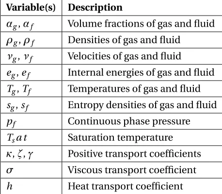
Table 2.1: Thermal-hydraulics parameters for the mass, momentum, and energy conservation equations.

Variable(s) Description

αg,αf Volume fractions of gas and fluid ρg,ρf Densities of gas and fluid

νg,νf Velocities of gas and fluid

e_g,e_f Internal energies of gas and fluid Tg,Tf Temperatures of gas and fluid sg,sf Entropy densities of gas and fluid pf Continuous phase pressure Tsa t Saturation temperature κ,ζ,γ Positive transport coefficients σ Viscous transport coefficient h Heat transport coefficient

2.2.1 Hydra-TH

Hydra-TH is a thermal-hydraulics code designed for use in nuclear reactor applications[39]. It was developed at Los Alamos National Laboratory for use in the CASL project. The hybrid finite volume/finite element multi-physics code was assembled with the goal of providing a detailed resolution of flow fields in a number of regimes and describing interactions with the reactor fuel assembly. Hydra-TH is capable of dealing with a number of problems in varying situations, including but not limited to:

• Crud-Induced Power Shift (CIPS)

• Crud-Induced Localized Corrosion (CILC) • Grid-To-Rod Fretting (GTRF)

• Departure from Nucleate Boiling (DNB).

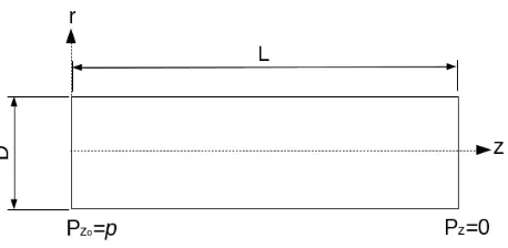
We consider laminar pipe flow in the setup depicted in Figure 2.2, wherepdescribes the pressure in the pipe,vz is the velocity along the length of the pipe,µis the kinematic viscosity of the fluid, andr denotes the radial coordinate. Neglecting body forces, the differential equation for Poiseuille flow in a laminar pipe flow is

∂p ∂z =µ

∂2_v

z ∂r2 +

1 r

∂vz ∂r

. (2.15)

The solution

vz(r) = 1 4µ d p d z D2

4 −r

2

,

to the differential equation (2.15) illustrates that the profile is quadratic in the radial direction. Here D represents the diameter of the pipe andd z is the length of the pipe over which the pressure drop d p occurs. It further follows that

d p d z =−

32Vµ

D2 , (2.16)

whereV is the average velocity over the pipe flow area. A dimensionless analysis reveals that d p

d z =− V2

2 ρ

Df, (2.17)

whereρandf respectively denote the fluid density and friction factor. We employ the valuesρ=977 kg/m3,D =0.0254 m, andµ=9.576×10−4kg/m·s. For laminar pipe flows, the friction factor is f =64/R e, whereR e=ρV D/µ. We note that the Reynolds numberR e must be less than 2300 to ensure laminar flow. Integrating equations (2.16) and (2.17), we obtain the pressure solutions

p(z) = −32Vµ(z−z0)

D2 +p(z0)

or

p(z) = −V

2

2

µ(z−z0) D

₆₄

R e

‹

+p(z0), (2.18)

wherep(z)andp(z0)are pressures at the upstream locationz and downstream locationz0in the

pipe. The choice ofz and z0 is arbitrary. As noted in equation (2.18), the pressure downstream

Figure 2.2: Configuration of laminar pipe flow.

We employ equation (2.17), along with the relations

V =R e·µ ρD and

f = 64 R e

for the average velocity and friction factor, to provide analytic relations to verify the accuracy of Hydra-TH for the considered flow regime.

We now discuss the Hydra-TH setup. To minimize effort when running the cases and minimize errors during the pre- and post-processing steps, we employ the automated strategy depicted in Figure 2.3(a). A three-dimensional mesh model of laminar flow in a pipe is run in Hydra-TH assuming constant inlet and outlet pressure at the pipe extremes. Figure 2.3(b) shows a typical hexahedron mesh used for these runs. This mesh is generated in Cubit by first meshing the circular surface (inlet side) with quadrilateral elements and then extruding these 2-dimensional elements along the direction of the pipe axis. We note that several tests were conducted with differing meshes; in particular, we employed a higher mesh density near the wall and higher mesh density near the center of the pipe. In general, better results were observed when the mesh density was finer at the center of the pipe.

(a) (b)

Figure 2.3: (a) Laminar flow schematic. (b) Hexahedron mesh for describing laminar flow in a pipe.

walls of the pipe are defined to have a no-slip condition.

The inlet pressure is calculated in the script using equation (2.18), assuming that the outlet temperature is zero. For these simulations, the diameter of the pipe is fixed at 0.0254 meters, and the length of the pipe is equal to 0.125·R e·D; i.e., two and a half times the developing length of the flow in the pipe. The time stepd t varied according to the Reynolds number and theC F Lnumber,

d t =∆z·C F Lm a x·ρ·D

R e·µ , (2.19)

where C F Lm a x ≈1.65. In all cases, a fully implicit Picard solution scheme is used to solve the coupled equations.

Details on the verification of the Hydra-TH code and the use of the code as a high-fidelity model for calibration of a lower-fidelity model will be discussed in Chapter 3.

2.2.2 COBRA-TF

areas, among others:

• Behavior of fuel rods and reactor decay heat • Heated and unheated conductors

• Two-phase heat transfer • Droplet breakup.

Within CTF, each of the three fields is modeled with its own set of mass, momentum, and energy conservation equations, together with a set of closure relations that makes possible the determination of the conservation parameters. The one exception to this rule is the liquid and droplet fields, which are assumed to be in thermal equilibrium, and therefore share a set of conservation equations. The conservation equations are formulated through one of two approaches: expression in 3-D Cartesian coordinate form, or a simplified subchannel approach which considers flow in only the axial and lateral directions. The equations are expressed in terms of finite-differences, then solved numerically over a mesh of finite volumes using the Semi-Implicit Method for Pressure-Linked Equations (SIMPLE).

Though CTF was not directly employed during the course of this dissertation, the goal of future calibration of CTF using a high-fidelity CFD code served as motivation in our development of the high-to-low framework of Part II. Work will soon be undertaken by another group to carry out this task.

Part II

CHAPTER

3

HIGH-TO-LOW FRAMEWORK

For many simulation models, it can be prohibitively expensive or physically infeasible to obtain a complete set of experimental data to calibrate model parameters. In such cases, one can alter-natively employ validated higher-fidelity codes to generate simulated data, which can be used to calibrate the lower-fidelity code. We employ an information-theoretic framework to determine the reduction in parameter uncertainty that is obtained by evaluating the high-fidelity code at a specific set of design conditions. These conditions are chosen sequentially, based on the the amount of information that they contribute to the low-fidelity model parameters. The goal is to employ Bayesian experimental design techniques to minimize the number of high-fidelity code evaluations required to accurately calibrate the low-fidelity model. This design scheme will be illustrated for several numerical examples in Section 3.4.

3.1

Design Framework

We employ the statistical model

dn=d`(θ,ξn) +δ(ξn) +"n(ξn), (3.1)

whered_`(θ,ξn)denotes the low-fidelity model, which depends on parametersθ∈Rp that we seek

to optimally calibrate using synthetic data constructed using a high-fidelity model. Hereξn ∈Ξ

denotes thent h_{design or evaluation strategy, whereΞdesignates the set of possible evaluation} strategies or experimental conditions. For the examples considered here,Ξis taken to be a discrete set of independent variable values. We denote potential discrepancy in the low-fidelity model by δ(ξn)and random measurement or discretization errors by"n(ξn).

When using mutual information measures to determine the next design pointξn, we employ independent and identically distributed (iid) Gaussian errors,"n(ξn)∼ N (0,σ2), whereσis a user-specified parameter. Throughout this work, we take 2σto be 10% of max_{i=1,···,n−1}d_h(ξi), where dh(ξi)is the high-fidelity solution evaluated using theξi design strategy. An alternative option is to inferσduring the calibration process. We note that this error assumption is commonly valid for measurement errors but will likely need to be modified for biases common to numerical errors.

For this investigation, we neglect model discrepancies and takeδ(ξn) =0. Discussion regarding the use of Gaussian processes,δ∼G P(0;λ_δ,ρ_δ), to quantifyδis provided in[3, 23, 24].

For a given designξn, thent h_{observation ˜d}

n, generated by the high-fidelity modeldh(ξn), is given by

˜

dn=dh(ξn) +"n˜ (ξn) (3.2) where potential numerical or measurement errors ˜"n(ξn)are assumed to be iid and normally distributed, ˜"n(ξn)∼ N(0, ˜σ2). Here ˜σis also a user-specified parameter. In this investigation, we again take 2 ˜σto be 10% of maxi=1,···,n−1dh(ξi)but note that, in general, ˜σcan differ fromσ. We employ the high-fidelity model (3.2) to generate the synthetic data used to calibrate the low-fidelity model.

The change in knowledge about the model parameters due to the addition of new synthetic or experimental data ˜dnis given by Bayes’ rule

p(θ|Dn) =

p(Dn|θ)p(θ) p(D_n) =

p(d˜n,Dn−1|θ)p(θ)

p(d˜n,Dn−1)

for the new data setDn={d˜n,Dn−1}. The goal in experimental design is to optimize the information

the proposed data as a result of measuring under design conditionsξn. Since ˜dnhas not yet been observed when we make a decision regarding the choice ofξn, we employ predictionsdn provided by the statistical model (3.1) to determineξn.

We employ Shannon entropy estimates to quantify the mutual information between the pro-posed observationdn and parameter valuesθ as in[60]. For a random variableΘhaving a corre-sponding densityp(θ)forθ∈Ω, the Shannon entropy is defined as

H(Θ) =−

Z

Ω

p(θ)log(p(θ))dθ

for the prior and

H(Θ|x) =−

Z

Ω

p(θ|x)log(p(θ|x))dθ

for the posterior distribution given datax. We define the utility of observing the high-fidelity code at conditionξn, perturbed by error, as

U(dn,ξn) =

Z

Ω

p(θ|dn,Dn−1)logp(θ|dn,Dn−1)dθ−

Z

Ω

p(θ|D_n−1)logp(θ|D_n−1)dθ, (3.3) which is a random function of unobserved datadn. By marginalizing over the domainD, the set of all unknown future observations, we obtain the average amount of information contributed by the proposed experimentξn. This yields

Edn[U(dn,ξn)] =

Z

D

U(dn,ξn)p(dn|Dn−1,ξn)d dn, (3.4) where the predictive distribution

p(dn|Dn−1,ξn) = Z

Ω

p(dn|θ,ξn)p(θ|Dn−1)dθ

substi-tute (3.3) into (3.4) and rewrite the expected utility as

Edn[U(dn,ξn)] =

Z

D

Z

Ω

p(θ,dn|Dn−1,ξn)log

p(θ,dn|Dn−1,ξn)

p(dn|Dn−1,ξn)

dθd dn

−

Z

D

Z

Ω

p(θ,dn|Dn−1,ξn)logp(θ|Dn−1)dθd dn

= Z

D

Z

Ω

p(θ,dn|Dn−1,ξn)log

p(θ,dn|Dn−1,ξn)

p(θ|D_n−1)p(dn|Dn−1,ξn)

dθd dn

= I(θ;dn|Dn−1,ξn). (3.5)

The result of (3.5) is the mutual informationI(θ;d_n|D_n−1,ξn)between the low-fidelity model parametersθand the proposed observationdnat design conditionξn. This gives a measure of the parameter uncertainty reduction provided by knowing the new data. We choose the optimal set of design conditionsξ∗_nto be the design that maximizes this quantity, namely

ξ∗

n=arg max_ξ

n∈Ξ

I(θ;dn|Dn−1,ξn).

The high-fidelity code is then evaluated using the design conditionξ∗_nand the resulting data ˜d_n is used to recalibrate the model parametersθ. This design is then eliminated from the design set, as design replication is not considered in this study. We note, however, that by allowing replication in design selections, one can formally quantify uncertainty in high-fidelity code calculations due to parameter variation; e.g., turbulence models in CFD codes. A basic implementation of our method is outlined in Algorithm 1.

3.2

kNN Estimate of Mutual Information

Algorithm 1Design Implementation

(1) DefineN, the number of samples to be used in either the Monte Carlo orkNN algorithms. (2) Initialize a list of pre-existing high-fidelity data,[(ξ1, ˜d1),(ξ2, ˜d2), ...,(ξr, ˜dr)].

(3) Define list of possible design conditions,[ξr₊1,ξr+2, ...,ξs].

(4) Ifr ≥1, run the DRAM algorithm (see Appendix A) to construct a chain{θi_}N

i=1of sizep×N

from the prior distributionp(θ|D_n−1), wherep is the number of parameters. Ifr=0; that is, there is no pre-existing data, construct a chain of sizep×N by sampling a proper priorp(θ) of choice.

(5) Send the chain{θi_{}to the Monte Carlo orkNN algorithms detailed in Sections 3.3.1 and 3.2.} (6) The Monte Carlo andkNN algorithms return a single design conditionξn. Append this value and the corresponding high-fidelity prediction ˜d_n=d_h(ξn) +"n˜ (ξn)to the previous data list to obtain

[(ξ1, ˜d1),(ξ2, ˜d2), ...,(ξr, ˜dr),(ξn, ˜dn)].

(7) Repeat steps 4-6 until all designs are used or a user-specified error tolerance is met.

ε(i)/2=||Xi−Xk(i)||∞, whereXk(i)represents thekth-nearest neighbor toXiin the chain{Xi}Ni=1

with respect to the sup norm, and determine the number of points in each marginal subspacen_θ andndthat lie withinε(i)/2 of the projected point; see Figure 3.1 for an example of this computation.

!

Xi

d

θ"

ε!

!

(i)

ε!

Figure 3.1: Calculation ofε(i),n_θ(i), andnd(i)for the casek=1 from[30]. Here we havenθ(i) =3

As detailed in[30], the mutual information can approximated by

I(θ;dn|Dn−1,ξn)≈ψ(k)−

1 N

–_N X

i=1

ψ(n_θ(i) +1) + N

X

i=1

ψ(nd(i) +1)

™

+ψ(N), (3.6)

whereψ(·)is the digamma function. A derivation of this quantity can be found in Appendix B. Algorithm 2kNN Method

(1) Fix value ofk (e.g.,k =6) and define number ofkNN vector elementsN (e.g.,N =2000). (2) For each potential designξn∈Ξ,

(a) Create a vector with dim(θ) +dim(d)rows andN columns

(i) In the first dim(θ) rows, draw N samples, {θi}Ni=1, from the prior distribution

p(θ|D_n−1).

(ii) In the next dim(d)rows, placed_n(ξn),i=1, ...,N. (iii) Normalize the data vector,

X=(diag(s−1)(X_i−µ) N_i=1

whereµ= [θ¯, ¯d]T is a(dim(θ) +dim(d))×1 vector of sample means ands= [s_θ,sd]T is the vector of sample standard deviations.

(b) For each sampleXi, identify thekth nearest neighbor,Xk(i), using the brute force or

ANN search algorithms.

(c) For each sampleX_i, computeε(i)/2=||X_i−X_k(i)||∞.

(d) For each sampleXi, computenθ(i) =# points inθ marginal space with at least one

coordinate within distanceε(i)/2 andnd(i) =# points ind marginal space with at least one coordinate within distanceε(i)/2.

(e) Estimate the mutual information:

I(θ;d_n|D_n−1,ξn)≈ψ(k)− 1

N

– _N X

i=1

ψ(n_θ(i) +1) + N

X

i=1

ψ(n_d(i) +1)

™

+ψ(N),

whereψ(·)is the digamma function. (3) Letξ∗be the design such that max

ξn∈Ξ

I(θ;dn|Dn−1,ξn) =I(θ;dn|Dn−1,ξ∗).

information may be calculated for a vector of possiblek values, and thek that yields the maximum mutual information value may be employed. In this work, we fixk =6 based on previous work done by Terejanu et al.[60], and save the analysis of a varyingk for future work.

3.2.1 ANN Search Algorithm

The process of identifying thekth_{-nearest neighbor requires computation times on the order of}

O(N2)using a brute force search, whereN is the number of data points, each consisting of a param-eter sample with a corresponding output as described in Section 3.2. We improve this by employing an approximate nearest neighbor (ANN) search algorithm[1, 37]. Within the ANN algorithm, the brute force search for the nearest neighbor is replaced by a hierarchical decomposition of space, dependent upon the construction of a balanced box-decomposition (BBD) tree; see[1]for back-ground on the BBD-tree data structure and details on its construction. By subdividing our space into a series of cells, each of which contains a subset of our data points, we can estimate the nearest neighbor by visiting cells in order of increasing distance outward from the query point.

We define the approximate nearest neighbor as follows. Given a setS of data points inRm, a

query pointq∈Rm, and an error toleranceε >0, a pointp∈Sis said to be an approximate nearest

neighbor ofqif

dist(p,q)≤(1+ε)dist(p∗,q),

wherep∗_{is the true nearest neighbor toq. That is,p is within errorεof the actual nearest neighbor} toq. We extend this to locating thekth-nearest neighbor; for 1≤k≤N, thekthapproximate nearest neighbor ofqis a data point whose relative error from the truekth-nearest neighbor is less thanε. With the ANN algorithm, we sacrifice total certainty that we have identified the true nearest neighbor, and accept an approximate nearest neighbor in its place. However, what we lose in accu-racy, we gain in computational savings, as the ANN algorithm allows us to identify an approximate nearest neighbor inO(NlogN)time in contrast to theO(N2_{)time that is required by thekNN brute}

force method. In addition,εcan be set to zero, in which case the ANN algorithm can correctly identify the truekth-nearest neighbor.