INVESTIGATION
Inference of Population Mutation Rate
and Detection of Segregating Sites
from Next-Generation Sequence Data
Chul Joo Kang1and Paul Marjoram
Department of Preventive Medicine, Keck School of Medicine, University of Southern California, Los Angeles, California 90089
ABSTRACTWe live in an age in which our ability to collect large amounts of genome-wide genetic variation data offers the promise of providing the key to the understanding and treatment of genetic diseases. Over the next few years this effort will be spearheaded by so-callednext-generationsequencing technologies, which provide vast amounts of short-read sequence data at relatively low cost. This technology is often used to detect unknown variation in regions that have been linked with a given disease or phenotype. However, error rates are significant, leading to some nontrivial issues when it comes to interpreting the data. In this article, we present a method with which to address questions of widespread interest: calling variants and estimating the population mutation rate. We show performance of the method using simulation studies before applying our approach to an analysis of data from the 1000 Genomes project.
W
E live in an era in which technology drives scientific discovery. This is very clearly demonstrated in molec-ular genetics, in which the development of technologies such as gene expression arrays and so-called SNP chips, to name just two examples, has led to a vast increase in the amount of genetic data at our disposal. Arguably, at this time our ability to interpret such data lags somewhat behind the technology. One of the most recent and exciting technologies to be placed at our disposal is next-generation sequence (NGS) platforms, in which enormous quantities of sequence data can be collected at reasonably low cost. In this article we focus on two applications of this technology: estimation of mutation rate and polymorphism detection.Our focus is partly motivated by a common use for NGS data in genome-wide association studies (GWAS). While GWAS have now identified a large number of loci at which polymorphism is associated with disease phenotypes, the overall amount of variance explained by these polymor-phisms is low (e.g., Manolioet al.2009; Frazeret al.2009). One explanation for the remaining variance, so-calleddark
matter, is the possible existence ofrare variants, polymorphic loci at which the minor allele has low frequency. With that in mind, in addition to the wish to answer general popula-tion genetics quespopula-tions, such as estimapopula-tion of mutapopula-tion rate, the investigator will often collect NGS data to identify poly-morphic loci at which to collect data in a follow-up study using a custom SNP array, say. This article presents a compu-tationally tractable method for estimating mutation rate and calling genotypes (and thereby detecting polymorphism).
NGS technology comes in a number of forms. Chief among these are the Illumina (San Diego, CA) Genome Analyzer, the 454 Genome Sequencers (Roche Applied Science, Basel, Switzerland), the SOLiD platform (Applied Biosystems, Foster City, CA), the Polonator (Dover Systems, Salem, NH), and the HeliScope Single Molecule Sequencer technology (Helicos, Cambridge, MA). While these methods differ in the details (see Shendure and Ji 2008 for a review), the data that are obtained have similar broad features. Es-sentially one obtains relatively short regions of sequenced DNA, so-called reads, either singly or in pairs drawn from opposite ends of a larger fragment of DNA. Typically these fragments are sequenced and then aligned using one of a number of possible algorithms [e.g., Mapping and Assem-bly with Quality (MAQ) (H. Liet al.2008) or Short Oligo-nucleotide Alignment Program (SOAP) (R. Liet al.2008)], but several key features are constant across platforms. First,
Copyright © 2011 by the Genetics Society of America doi: 10.1534/genetics.111.130898
Manuscript received May 20, 2011; accepted for publication July 14, 2011
1Corresponding author: Department of Preventive Medicine, CHP234, Keck School
the reads are short (35–400 bp, depending upon platform); second, for that reason, alignment to a reference sequence is challenging; third, genotyping error rates vary along the read, typically increasing as we move along the read (mod-ulo some variation from that trend that may exist at the beginning of the reads). In this article we do not focus on the issue of alignment—our method is designed to be ap-plied to reads postalignment.
While these technologies are new, a number of ap-proaches already exist for the analysis of the resulting data. In the context of estimating mutation rate, thefirst method was that of Hellmannet al.(2008). While their method was developed for shotgun-sequencing data, in which error rates are lower, it can nonetheless be applied to NGS data, albeit at some loss of performance. A similar approach was taken by Jiang et al. (2008), where robustness to issues such as genotyping errors or biased amplification was examined more explicitly. Furthermore, a wide variety of methods drawn from related topics also exist. Examples of this range from the extremely elegant and simple estimator due to Watterson (1975), to the more computationally intense methods of Griffiths and Tavaré (1994) and Kuhner et al. (1995). However, none of these methods were developed for NGS data, and, for example, they fail to allow for the possibility of genotyping error. Methods for estimating mu-tation rate in the presence of genotyping errors do exist, for example, approaches based upon considering nonsingleton variants (Knudsen and Miyamoto 2009), but these do not exploit the particular properties of NGS data.
In this article we use thecoalescentas a model for geno-type data for a sample of individuals drawn from a popula-tion. The coalescent wasfirst formalized by Kingman (1982 a,b,c) and has become the most widely used model for pop-ulation genetics data. For accessible introductions see Wake-ley (2008) or Hein et al. (2005). Several algorithms now exist for detection of polymorphic sites for NGS data. Li and Leal (2009) developed a Bayesian method for comput-ing individual genotype likelihood values from NGS data. There are also approaches that combine the resequenced data of the samples for better SNP calling. For example, Bansalet al.(2010) used a method containing a population error correction term to avoid systematic sequencing errors. Such methods were used in the 1000 Genomes Project Con-sortium (2010). After giving methodological details of our approach we demonstrate performance via a series of simu-lation studies before applying it to data from the 1000 Genomes Project and comparing to results from two popular algorithms: samtools and GATK.
Methods
Overview of the E–M algorithm
We assume we have read data that have been aligned to a reference sequence and, in the simplest form of our algorithm, that we have known (or estimated)
position-specific error rates. Our goal is to compute individual genotype likelihoods for a sample of size n,i.e., the proba-bility of the genotype for each site for each member of the sample. For computational tractability our method ignores information due to linkage disequilibrium (seeDiscussion).
Our method is an E–M algorithm that explores possible values for Q and the genotype data while producing the maximum-likelihood estimate of the population mutation rate 4Nem = Q, where Ne is the effective population size andm is the mutation rate per base per individual. We ini-tialize using an arbitrarily chosen value of Q = 0.001. In outline the algorithm proceeds as follows:
1. Expectation step: Conditional on the currentQ-value and the observed read data, we calculate the expected num-ber of polymorphic sites,E(S).
2. Maximization step: UpdateQon the basis ofE(S).
In analyses in which we also wish to infer error rates, those error rates are updated in step 2, along with Q.
We iterate the above steps 100 times and then, using the
final estimated Q, the posterior probability of being poly-morphic is computed for each site. For each site that is predicted to be polymorphic, the genotype and output, for each individual in the sample, are inferred. While our method is computationally intense, for the examples given in this article, in which we simulate 20 diploid samples over a 100-kb region, the run time is short: 1 min for estimation ofQor 30 min with coestimation ofQand error rates. Run time is approximately linear with the length of region being analyzed.
We now give more details on each of the above steps.
Calculation of the likelihood
We begin by deriving the likelihood ofQconditional on the read data. LetR= {R1,R2,. . .,Rn} be the set of read data
across all sites (i.e., all base positions) over all samples and letGdenote the unobserved genotypes across all sites. Using Bayes’theorem, the probability ofQgiven the read data for a sample is
ProbðQjRÞ ¼ProbðRjQÞProbðQÞ
ProbðRÞ : (1)
The likelihood of read data R given Q is the summation of the joint probabilities over all possible underlying genotypes:
LðQÞ ¼X
G
ProbðRjGÞProbðGjQÞ: (2)
By ignoring linkage disequilibrium we can compute a composite likelihood (cf. Hudson 2001) by multiplying the likelihoods at each site:
LðQÞ Y
i
X
g
where i indexes sites, g denotes the sample genotypes at a given site, and Prob(Ri|g) is set to 1 if Ri does not
overlapg.
Calculation of Equation 3 requires derivation of the terms Prob(Ri|g) and Prob(g|Q). We begin by deriving Prob(Ri
|g).
Let r be the set of read data at a given position in the genome for a given individual,rkrefer to thekth element of
r, ande(rk) be the error rate of the base called at this
posi-tion for rk. This can be estimated using quality scores, or
from external estimates of read accuracy. While it is gener-ally the case that error rate can be reasonably assumed to vary across positions within a read, but to be constant across reads at each position, we do not make this restric-tion here. Leta0be the base at this position in the reference sequence and a1 denote a possible variant type. We now compute the individual genotype likelihoods for each pos-sible genotype. The pospos-sible genotypes can be categorized as homologous consensus/consensus, heterozygous consen-sus/variant, and homologous variant/variant. To improve computational efficiency we assume at most a single muta-tion at each posimuta-tion in the ancestry of the sample, as is the case with the so-called infinite sites mode, for example. Thus, we write
Probðrjaj;ajÞ
Q
rk¼aj
ð12eðrkÞÞ·
Q
rk6¼aj ðeðrkÞÞ
Probðrja0;a1Þ Q
rk¼a0
1
2ð12eðrkÞÞ þ 1 2eðrkÞ
· Q rk¼a1
1
2ð12eðrkÞÞ þ 1 2eðrkÞ
¼1 2
jrk¼a0jþjrk¼a1j
(4)
We then compute the joint likelihood of the sample geno-types at a given position by multiplying these individual likelihoods.
Next we derive Prob(g| Q). The prior probabilities for each genotype are calculated from the expected allele fre-quency spectrum under the coalescent model with constant population size or expanding population size (as appropri-ate). The joint prior probabilities of each genotype are then approximated from the expected allele frequency spectrum (Griffiths and Tavaré 1998).
Probðgð0ÞjQÞ ¼12Q· P n21
j 1
j
ProbðgðmÞjQÞ ¼ ð12Probðgð0ÞjQÞÞm1
0 @Xn21
j 1 j 1 A 21 n m 21
ðm.0Þ
where g(m) represents a genotype with m mutant alleles across the sample.
Estimation ofQ
The value of Qmaximizing the likelihood is derived using an E–M algorithm. The derivative of the likelihood function (3) is
LðQÞ9¼X
i
Pn21
m¼1ProbðRijgðmÞÞProbðgðmÞjQÞ
Pn21
m¼0ProbðRigðmÞÞProbðgðmÞQÞ
0 @n·X
n21
j 1 j 1 A 21 : (5)
From this we see that in the expectation step we will esti-mate the expected number of polymophic sites, by summing the probability of each site being polymorphic, where that calculation is performed using the existing estimate ofQat each site:
SE¼ X
i
Pn21
m¼1ProbðRijgðmÞÞProbðgðmÞjQÞ
Pn21
m¼0ProbðRigðmÞÞProbðgðmÞQÞ
(6)
We then re-estimateQ, per Equation 5, which can be under-stood as Watterson’s estimator ofQbut using the expected (rather than observed) number of polymorphic sites.
Unknown error rates
In its simplest form, our method requires the error rates of the resequencing process as input. While these will generally be available (via quality scores for example) we note that, if not, our method can coestimate either a single overall error rate E* or a vectorEof position-specific error rates, while estimating Q and calling polymorphism. In this case we model the error rates as growing exponentially along the read, which reflects the generally observed behavior. For example, the likelihood that (3) is rewritten as
LðQ;EÞ Y
i
X
g
ProbðRijg;E*ÞProbðgjQÞ
and the vector of position-specific error rates,E= {E1,E2, ..., EL} (say), can be estimated within the E–M algorithm
Ek¼
P
iPgagi;k·lðg;iÞ
P
i
P
gni;k·lðg;iÞ¼
P
iPgagi;k·lðg;iÞ
P
ini;k ;
where agi;k is the number of reads that do not match geno-typegat siteiin the resequencing positionkandni,kis the
total number of reads at sitei.l(g,i) is the posterior prob-ability of genotype gat sitei:
lðg;iÞ ¼PProbðRijg;EÞProbðgjQÞ
gProbðRig;EÞProbðgQÞ
Ek
P
ia gð0Þ
i;k ·lðgð0Þ;iÞ
P
ni;k·lðgð0Þ;iÞ :
After estimation of error rate at each read position, wefit an exponential curve to derive smoothed estimates of position-specific error rates.
Output of polymorphic sites
At the conclusion of our algorithm, we calculate the pos-terior probability of polymorphism at each site by condi-tioning on the final estimated Q-value and computing the posterior probability of polymorphism for each site as
ProbðpolymorphicjRiÞ ¼
P
polymorphic gProbðRijgÞProbðgjQÞ
P
gProbðRigÞProbðgQÞ
:
Since all sites will have a nonzero probability of being polymorphic, but for most sites that probability will likely be small, we adopt the following heuristic. We use a predeter-mined threshold T. If the posterior probability of polymor-phism at a site exceedsT, that site is reported as a candidate polymorphic site. In the examples in this article we useT= 0.9. For sites that are predicted to be polymorphic, the ge-notype with the highest posterior probability is then output for each individual.
Results
Simulation of data
For all analyses in the article that are based upon simu-lated haplotypes, we simusimu-lated over a 100-kb region using Hudson’s coalescent simulator ms (Hudson 2002) under a constant population-size model. We assume sequencing occurs on an individual level. Twenty diploid genomes were
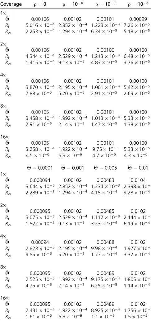
Table 1 The mean estimatedQvalue and RMSEs (see text for definitions) for varying population parameters
Coverage r¼0 r¼1024 r¼1023 r¼1022
1· ^
Q 0.00106 0.00102 0.00101 0.00099
Rt 5.016·1024 2.852·1024 1.223·1024 7.26·1025
Rw 2.253·1024 1.294·1024 6.34·1025 5.18·1025
2· ^
Q 0.00106 0.00102 0.00100 0.00100
Rt 4.344·1024 2.529·1024 1.213·1024 6.48·1025
Rw 1.415·1024 9.13·1025 4.83·1025 3.76·1025
4· ^
Q 0.00106 0.00102 0.00101 0.00100
Rt 3.870·1024 2.195·1024 1.061·1024 5.42·1025
Rw 7.88·1025 5.20·1025 2.91·1025 2.69·1025
8· ^
Q 0.00105 0.00102 0.00101 0.00100
Rt 3.458·1024 1.992·1024 1.013·1024 5.33·1025
Rw 2.91·1025 2.14·1025 1.47·1025 1.38·1025
16· ^
Q 0.00105 0.00102 0.00101 0.00100
Rt 3.258·1024 1.922·1024 9.75·1025 5.33·1025
Rw 4.5·1026 5.3·1026 4.7·1026 4.3·1026
Q¼0.0001 Q¼0.001 Q¼0.005 Q¼0.01 1·
^
Q 0.000094 0.00102 0.00483 0.0104
Rt 3.644·1025 2.852·1024 1.234·1023 2.398·1023
Rw 2.289·1025 1.294·1024 4.15·1024 9.28·1024
2· ^
Q 0.000095 0.00102 0.00485 0.0102
Rt 3.075·1025 2.529·1024 1.112·1023 2.144·1023
Rw 1.522·1025 9.13·1025 3.23·1024 6.19·1024
4· ^
Q 0.00094 0.00102 0.00488 0.0102
Rt 2.823·1025 2.195·1024 9.98·1024 1.927·1023
Rw 9.55·1026 5.20·1025 1.77·1024 3.32·1024
8· ^
Q 0.000095 0.00102 0.00489 0.0102
Rt 2.525·1025 1.992·1024 9.175·1024 1.805·1023
Rw 4.75·1026 2.14·1025 6.25·1025 1.14·1024
16· ^
Q 0.000095 0.00102 0.00489 0.0102
Rt 2.431·1025 1.922·1024 8.925·1024 1.756·1023
Rw 1.61·1026 5.3·1026 1.1·1025 1.5·1025
Top:Q¼0.001 whilervaries; bottom:Qvaries whilerisfixed at 1024. In all cases,
25 diploid samples were generated on the basis of constant population size model.
Table 2 The mean estimatedQvalue and RMSEs for varying sample sizes,n
Coverages n¼10 n¼25 n¼50
1· ^
Q 0.00099 0.00102 0.00097
Rt 2.907·1024 2.852·1024 2.573·1024
Rw 1.483·1024 1.294·1024 1.043·1024
2· ^
Q 0.00099 0.00102 0.00097
Rt 2.614·1024 2.529·1024 2.304·1024
Rw 1.106·1024 9.13·1025 7.09·1025
4· ^
Q 0.00099 0.00102 0.00097
Rt 2.395·1024 2.195·1024 1.996·1024
Rw 6.28·1025 5.20·1025 3.84·1025
8· ^
Q 0.00099 0.00102 0.00098
Rt 2.206·1024 1.992·1024 1.845·1024
Rw 1.97·1025 2.14·1025 1.66·1025
16· ^
Q 0.00099 0.00102 0.00098
Rt 2.123·1024 1.922·1024 1.773·1024
Rw 5.7·1026 5.3·1026 4.1·1026
HereQ¼ 0.001 andr¼1024in all cases. Twenty-five diploid samples were
formed by random pairing of haplotypes. We then generated paired-end NGS data, with reads occurring as a Poisson pro-cess, each end consisting of a read of 35 bases and the distance between ends being Normally distributed with mean 500 and standard deviation of 20. Unless otherwise specified the NGS data were generated with an overall av-erage error rate of 0.005, but with error rates increasing as the read is traversed. Specifically, the error rate at read po-sitioniwas assumed to be
Ei¼eaþib; (7)
with b= 0.1.
Estimation ofQfrom simulated data
From the simulated data set we estimate Q for a range of coverages per diploid and/or a range of sample sizesn. For each combination of parameters (mutation rate, Q, recom-bination rate,r, coverage,X, and diploid sample size,n) we simulated 100 data sets. We assumed that the position-spe-cific error rates were known. Table 1 shows results for a va-riety of values ofrandX.
In the top half of Table 1Qisfixed at 0.001 andrvaries, while in the bottom half Qvaries whileris fixed at 1024. We show the average of the estimated Q-values, Q^, along with,Rt, defined as the root mean squared error (RMSE) of the ratio of our estimate ofQcompared to the trueQvalue
(we normalized by dividing byQto ease interpretation). For benchmark purposes, we also compare our estimate of Q, based upon the resequencing data, to that obtained by ap-plying Watterson’s estimator Watterson (1975) to the true (and, in fact, unobserved) haplotype data. For this purpose we report (Rw), the root mean squared error of the ratio of Watterson’s estimate ofQcompared to the trueQ.Rw rep-resents a good estimate of the limit of what is attainable
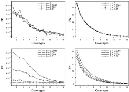
Figure 1 The false-positive rates (FP) and false-negative rates (FN) for polymorphic site detection as a function of minor allele frequency. Whenrvaries (top two plots),Qisfixed at 0.001; whenQvaries (bottom two plots),risfixed at 1024.
due to the stochastic noise within the coalescent process itself (since Watterson’s estimate is known to be a good estimator ofQ, and we apply it here to the unobserved true genotypes).
The estimates ofQare close to the true value ofQfor all combinations of parameters, even at 1· coverage. As expected, RMSE values are bigger when coverage is low. We also see that Q is slightly overestimated for lower re-combination rates, which is a reflection of the increased variance of our, or any other estimator of Q as LD in the data increases.
In the lower part of Table 1 we show results for a range of
Q-values withrfixed. Once again the estimator appears to perform very well in all cases.
Next, in Table 2, we show results as a function of sample size for scenarios in which Q = 0.001 andr = 1024. Per-formance is robust to change of sample sizen, with RMSEs decreasing asnincreases, as is expected.
Detection of polymorphic sites
In Figure 1 we show the positive rate, FP, and false-negative rate, FN, as a function of coverage. For a range of
Q2andr-values we show the percentage of sites called as segregating that are not in fact polymorphic, FP (y-axis), against coverage X (x-axis). We also show plots for the FN rate. We see that both the FP and FN rates are reduced as coverages increases, as would be expected. Both FP and FN are robust to changes in recombination rate, but both are sensitive to changes in mutation rate. The power to detect polymorphic sites is affected by minor allele fre-quency (MAF). In Figure 2, we see that our method results in good detection rates for common variants (MAF.0.05) given reasonable coverage (say 4·), but that, unsurpris-ingly, many rarer variants are missed, especially with lower coverages.
Given that our method is based on the constant pop-ulation size model, it is important to explore robustness to departures from that assumption. We focus on situations in which, as is common, population size is growing. Two data sets were simulated under an exponentially growing pop-ulation size, where the poppop-ulation size at timetunits back into the past,N(t), is modeled asN(t) =N0e–rt, whereN0is the current population size andris the exponential growth rate. Table 3 shows the false-negative rates of polymorphic
site calling for three different growth rates. Since exponen-tial growth leads to there being more rare variants, variation on average become harder to detect.
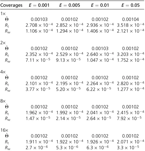
Effects of resequencing error rate
We also explored the effect on performance of changes to the overall base-calling error rate and to (read) position-specific base-calling error rates. Assuming exponentially distributed position-specific error rates, per Equation 7, we
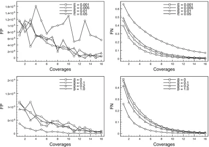
first explore changes to the overall rate, while settingb= 0.1 (both are assumed known). Table 4 shows that perfor-mance is robust to this change. However, the false-positive and -negative rates do grow higher as the overall error rate increases, as might be expected (Figure 3).
Second, we assumed the overall error rate is fixed, but changedb, reflecting varying degrees of degradation of call-ing accuracy along the reads. Once again our method is robust to this change (Table 5) but again the FP and FN rates are affected (Figure 3).
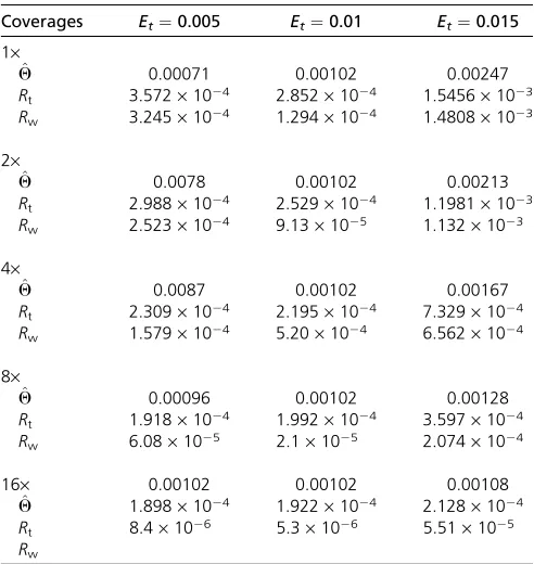
It is also of interest to see how performance is affected if incorrect error rate estimates are used during the analysis. This introduces biases to the estimatedQ-values. When the actual error rate is lower than the assumed error rate,Qis underestimated, and when the actual error rate is higher than assumed, Q is typically overestimated. These biases decreased as the level of coverage increases (Table 6).
It is also possible to jointly estimate (i) average error rate,Et, and associated exponential parameterb, and (ii)Q. Table 7 shows results for this case. For all coverage levels, the estimated values are close to the true values, and
Table 3 The effect of population growth on polymorphic site detection
Coverages r¼0 r¼1024 r¼1023
1· 0.4700 0.5390 0.6861
2· 0.3246 0.3804 0.5194
4· 0.1804 0.2146 0.3159
8· 0.0564 0.0719 0.1092
16· 0.0063 0.0076 0.0105
Population data were simulated with different exponential growth rates rand current population size N0¼10,000 (see text for details). We report the false
negative rate.
Table 4 The mean of estimatedQand RMSEs from resequencing data simulated with differing average error rates
Coverages E¼0.001 E¼0.005 E¼0.01 E¼0.05
1· ^
Q 0.00103 0.00102 0.00102 0.00104
Rt 2.708·1024 2.852·1024 2.936·1024 3.518·1024
Rw 1.106·1024 1.294·1024 1.406·1024 2.121·1024
2· ^
Q 0.00102 0.00102 0.00103 0.00102
Rt 2.352·1024 2.529·1024 2.640·1024 3.203·1024
Rw 7.11·1025 9.13·1025 1.047·1024 1.752·1024
4· ^
Q 0.00102 0.00102 0.00102 0.00102
Rt 2.101·1024 2.195·1024 2.264·1024 2.820·1024
Rw 3.77·1025 5.20·1025 6.22·1025 1.277·1024
8· ^
Q 0.00102 0.00102 0.00102 0.00102
Rt 1.962·1024 1.992·1024 2.041·1024 2.415·1024
Rw 1.47·1025 2.14·1025 2.64·1025 7.92·1025
16· ^
Q 0.00102 0.00102 0.00102 0.00102
Rt 1.911·1024 1.922·1024 1.926·1024 2.071·1024
Rw 2.7·1026 5.3·1026 6.3·1026 3.3·1025
accuracy of polymorphic site detection is much the same as for the analysis that assumes the true error rate (data not shown).
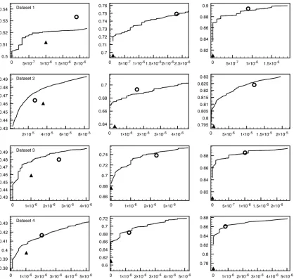
Comparison with other polymorphic site-detection methods
We next use simulated data to compare performance of our method, when focused on polymorphism detection, to that of other detection tools (samtools version 0.1.12) (Li and Leal 2009), and GATK Unified Genotyper (v. 1.0) (Mckenna et al. 2010). To do this we created four 100-kb data sets, each containing 40 diploid samples, using four different mu-tation parameters (Q = 0.00001, 0.0001. 0.0002, and 0.0005). This resulted in data with 52 (data set 1), 531 (data set 2), 915 (data set 3), and 2482 polymorphic sites (data set 4), respectively. We then simulated 100 replicate sets of read data at three different coverages (1·, 4·, 8·). The simulated reads were then mapped with BWA (Burrows-Wheeler Alignment Tool) (Li and Durbin 2009). We then analyzed each of these data sets using our method, sam-tools, and GATK using default parameter values for the latter two methods. Figure 4 shows a summary of results over the 100 replicates. Results for our method are a function of the threshold, T; for calling a polymorphism, this results in a curve of results, as a function ofT, compared to the single datapoint for the other two approaches. For all data sets and coverages, our method shows good polymorphic site detec-tion rate.
Analysis of 1000 Genomes Project data
We also applied our method to a 10-Mb region (16 Mb26 Mb) on chromosome 21 from the 1000 Genomes Project data. We use only the Illumina data; for the purpose of sim-plicity, data from other platforms are ignored. Aligned NGS data from 57 African samples (Yoruba), 51 European sam-ples [CEPH (Centre d’Etude du Polymorphisme Humain)], and 58 Asian samples [CHB (Chinese from Beijing) + JPN (Japanese)] were used. The analyzed data are from the Low Coverage Pilot project, in which the whole genome was se-quenced at low coverage (the average coverage in the ana-lyzed region is 3.4·). To improve computational efficiency and allow for local variation of population mutation rate, we divided the 10-Mb region into 100-kb subregions (with no overlap), and analyzed each separately. For each subregion,
Q-values were estimated and polymorphic sites and MAFs were predicted. We analyzed data from each population separately. For quality control, when applying our genotyp-ing algorithm, reads with more than two mismatches to consensus sequence or lower mapping quality score (, 30) were not included in the analysis. The sequencing error rate per single read per site was inferred from the quality score, as in Cock et al. (2010). To improve comparability between results from our method, and those from 1000 Genomes, we use a probability threshold of T= 0.9, as is commonly used in similar analyses of 1000 Genomes Data (cf. Liet al.2011). Results are shown in Figure 5.
As expected, the estimated Qfrom the African data are bigger than from other populations. The average values over the region for the African, European, and Asian populations
are 0.00112, 0.000742, and 0.000650, respectively. The lo-cal variation of estimated Q-values between populations is highly correlated. The non-African populations show highest correlation (R2= 0.727). The correlation between African and non-African populations is also high (African-European R2= 0.560 and African-AsianR2= 0.489) but some regions show differences. (17.9–18.1 Mb, 21.6–21.7 Mb, 24.1–24.4 Mb, and 25.3–25.5 Mb). These lower estimates for the non-African populations may be evidence of local selection, but might also reflect systematic differences in data production across centers, or simply noise.
Figure 6 shows a summary of our polymorphic site calls. First we show the number of polymorphic sites detected. Second, we calculate and report the expectation of the minor allele frequency, using the posterior genotype probabilities at all sites that are called polymorphic. More polymorphic sites are inferred from the African population than from the Asian or European populations. The mean MAF at polymorphic sites from the African, Asian, and Eu-ropean populations are about 0.145, 0.189, and 0.169, re-spectively. This is bigger than the expected MAF derived from even a constant population size model (0.053). This reflects an ascertainment bias due to the diffculting of detecting rare variants. The average MAF of population-pri-vate polymorphic sites is 0.048 and is much lower than poly-morphic sites common to all three populations (0.22), again as would be expected (assuming that private polymorphisms are likely to have arisen more recently).
For the Yoruban population we compared our poly-morphic site calls to those in dbSNP (version 129) and to calls from the 1000 Genomes Project (Figure 7). A compar-ison between estimated MAFs of novel and known variants shows that the polymorphic sites reported in dbSNP are relatively common variants. About 82% of variable sites from the 1000 genome study are inferred as polymorphic by our method. Our method infers 2410 more known sites than the 1000 Genomes Project. As a quality check of poly-morphic site calling, we calculated the transition/transver-sion ratios (ts/tv) using the predicted genotypes at sites that were detected as polymorphic. The overall ts/tv ratio using calls from our algorithm is 2.28, but the ts/tv ratio of novel sites is significantly lower (1.83), suggesting a greater num-ber of false positives at novel sites.
Our method can simultaneously estimate resequencing error rates. We therefore estimated error rates for the 1000 Genome Project data. The error rate of each read position is
Table 5 The mean of estimatedQ, and RMSEs, from resequencing data with differing error rate distributions along the read
Coverages b¼0 b¼0.1 b¼0.2 b¼1.0
1· ^
Q 0.00103 0.00103 0.00102 0.00102
Rt 2.949·1024 2.852·1024 2.686·1024 2.292·1024
Rw 1.382·1024 1.294·1024 1.109·1024 6.59·1025
2· ^
Q 0.00102 0.00102 0.00102 0.00102
Rt 2.544·1024 2.529·1024 2.375·1024 2.138·1024
Rw 9.57·1025 9.13·1025 7.46·1025 4.31·1025
4· ^
Q 0.00103 0.00102 0.00102 0.00102
Rt 2.222·1024 2.195·1024 2.130·1024 2.000·1024
Rw 5.40·1025 5.20·1025 4.17·1025 1.92·1025
8· ^
Q 0.00102 0.00102 0.00102 0.00102
Rt 2.024·1024 1.992·1024 1.970·1024 1.911·1024
Rw 2.36·1025 2.14·1025 1.69·1025 6.2·1026
16· ^
Q 0.00102 0.00102 0.00102 0.00102
Rt 1.916·1024 1.922·1024 1.913·1024 1.906·1024
Rw 5.2·1026 5.3·1026 3.8·1026 1.4·1026
Data sets were simulated withQ¼0.001 andr¼1024. The average error rateEis fixed at 0.005.
Table 6 The mean of estimatedQfrom resequencing data with differing average resequencing error rateEt
Coverages Et¼0.005 Et¼0.01 Et¼0.015
1· ^
Q 0.00071 0.00102 0.00247
Rt 3.572·1024 2.852·1024 1.5456·1023
Rw 3.245·1024 1.294·1024 1.4808·1023
2· ^
Q 0.0078 0.00102 0.00213
Rt 2.988·1024 2.529·1024 1.1981·1023
Rw 2.523·1024 9.13·1025 1.132·1023
4· ^
Q 0.0087 0.00102 0.00167
Rt 2.309·1024 2.195·1024 7.329·1024
Rw 1.579·1024 5.20·1024 6.562·1024
8· ^
Q 0.00096 0.00102 0.00128
Rt 1.918·1024 1.992·1024 3.597·1024
Rw 6.08·1025 2.1·1025 2.074·1024
16· 0.00102 0.00102 0.00108
^
Q 1.898·1024 1.922·1024 2.128·1024
Rt 8.4·1026 5.3·1026 5.51·1025
Rw
Data were simulated withQ¼0.001,r¼1024, andr¼0.1.
Table 7 The mean of co-estimatedQ, average error rateEandb
Coverages Q^ E b
1· 0.00103 0.00499 0.1005
2· 0.00103 0.00500 0.1001
4· 0.00102 0.00500 0.1000
8· 0.00102 0.00500 0.1000
16· 0.00102 0.00500 0.1000
estimated from data for the Yoruban population, using a constant-sized population model. Results are shown in Fig-ure 8. Our estimates are highly correlated with the error rate reported in 1000 Geomes; however, our estimated error rates show a systematic tendency to be lower than those derived during the 1000 Genomes analysis. This may reflect differences in the preprocessing of the read data. For exam-ple, in our analysis all reads with two or more mismatches were excluded.
Discussion
In this article we have presented a method for both (i) estimation of overall mutation rateQ, and (ii) calling poly-morphic sites, within a region for which NGS data have been collected. The posterior probability of a site being polymor-phic is computed for each site, along with an estimate ofQ. If position-specific error rates are not known, or the accuracy
of estimates of these are in doubt, our method can also estimate those error rates within its likelihood framework. However, in general, estimation of error rates is unlikely to be needed. Our method appears to work well, in part at least because it exploits the coalescent model to leverage power when genotyping jointly across multiple individuals.
There are at least three sources of information that can be used when calling genotypes at a given locus,L, for a given individual,I, (say):
1. The read data for that individual at that position; 2. the data for other individuals at that position; and 3. the data at other positions.
Each of these three sources could be used to inform either genotype calls or determination of whether the locus is polymorphic. When interpreting thefirst source of informa-tion, the key question to address is“Do the data result from genuine heterozygosity within that individual, or are they a
result of base-calling errors from the sequencing platform?” A variety of methods exists for dealing with this issue, such as those compared in this article. Intuitively speaking, the likelihood of interpreting a set of read data at L for I as evidence for heterozygosity should increase if polymorphism at that locus is also observed in other individuals. (Once we have seen a variant allele atLwe are more likely to see it at that location in subsequent individuals.) This information is exploited by our algorithm. Patterns of linkage disequilib-rium (LD) are also informative regarding genotyping (and hence calling of polymorphism). Loosely speaking, we should be more likely to call a polymorphism atLif the data support a pattern of polymorphism atLthat would be in LD with other nearby loci. Detailed modeling of patterns of LD is a complex issue, generally implying significant computa-tional complexity.
It is also worth noting that LD information will not greatly help to detect a polymorphism that has not already been observed in an existing sample. For these reasons we omit it from the present method, but our results show that
our method performs well despite making this simplification (a choice that ensures computational tractability). Nonethe-less, it has been successfully exploited using a number of different underlying probabilistic models, in algorithms such as fastPHASE and Li and Stephens’ PAC method) (Li and Stephens 2003; Scheet and Stephens 2006). However, appli-cations to SNP data are of much lower dimension than to NGS data, and it is not clear how tractable those methods might remain when applied to NGS data, where we are looking at many millions of bases. Neither will it be straight-forward to allow for the specific error structure of read data, in which, broadly speaking, error rates increase as we move along the read. It is reasonable to think that algorithms that eventually also include this third source of information will result in a further improvement in performance over this method, but the computational challenges will be sig-nificant. Our method exploits the first two sources of
Figure 5 The distribution ofQover the 10-Mb region of chromosome 21 of the African, European, and Eastern Asian populations from 1000 genome sequence data.
Figure 6 The number of inferred polymorphic sites, mean of the expected MAF (in parentheses), and ts/tv ratio (in italics) in each popula-tion in the 10-Mb region of chromosome 21.
Figure 7 A comparison of inferred polymorphic sites in the African pop-ulation using our analysis, calls from the 1000 Genomes Project, and known polymorphic sites from dbSNP. We show the number of inferred polymorphic sites, mean of the expected MAF, and the ts/tv ratio.
information and already requires significant computational resources, even though it does not use LD information for genotyping. However, we have shown that it results in good ability to accurately infer mutation rates and to call genotypes.
In this article, our method was applied to simulated data in which we assumed that reads had been aligned without error. This is not, of course, the case with real data (e.g., our analysis of the 1000 Genomes data) or for the analysis in Figure 4, in which read alignment algorithms were applied to simulated read data. Our method does work well in these more realistic scenarios, but it is important to note that the read alignment process can be expected to induce biases in estimation of mutation rate and/or polymorphism calling, for example, in regions in which alignment is difficult (e. g., near indels). Since most alignment approaches discard reads that have a nontrivial number of mismatches, a down-ward bias in the estimation of Qcan be expected to occur (since some of these mismatches presumably represent true polymorphism.)
Software for implementation of our method is available upon request from the authors. We note that, as well as outputting most likely genotype calls for loci that are determined to be polymorphic, the algorithm can be used to output posterior genotype probabilities at those loci. This would allow for explicit incorporation of uncertainty in genotype calls to be incorporated in subsequent analyses, such as genome-wide association studies.
Acknowledgments
The authors gratefully acknowledge funding from National Institutes of Health award 3R01 MH084678 and the helpful comments of two reviewers.
Literature Cited
1000 Genomes Project Consortium, 2010 A map of human ge-nome variation from population-scale sequencing. Nature 467: 1061–1073.
Bansal, V., O. Harismendy, R. Tewhey, S. S. Murray, N. J. Schork et al., 2010 Accurate detection and genotyping of snps utiliz-ing population sequencutiliz-ing data. Genome Res. 20: 537–545. Cock, P. J. A., C. J. Fields, N. Goto, M. L. Heuer, and P. M. Rice,
2010 The sanger fastqfile format for sequences with quality scores, and the solexa/illumina fastq variants. Nucleic Acids Res. 38: 1767–1771.
Frazer, K., S. Murray, N. Schork, and E. Topol, 2009 Human ge-netic variation and its contribution to complex traits. Nat. Rev. Genet. 10: 241–251.
Griffiths, R., and S. Tavaré, 1994 Ancestral inference in popula-tion genetics. Stat. Sci. 9: 307–319.
Griffiths, R., and S. Tavaré, 1998 The age of a mutation in a gen-eral coalescent tree. Stoch. Models 14: 273–295.
Hein, J., M. Schierup, and C. Wiuf, 2005 Gene Genealogies, Vari-ation and Evolution. Oxford University Press, Oxford.
Hellmann, I., Y. Mang, Z. Gu, P. Li, F. De La Vega et al., 2008 Population genetic analysis of shotgun assemblies of ge-nomic sequence from multiple individuals. Genome Res. 18: 1020–1029.
Hudson, R., 2001 Two-locus sampling distributions and their ap-plication. Genetics 159: 1805–1817.
Hudson, R., 2002 Generating samples under a Wright–Fisher neutral model. Bioinformatics 18: 337–338.
Jiang, R., S. Tavaré, and P. Marjoram, 2008 Population genetic inference from resequencing data. Genetics 181: 187–197. Kingman, J., 1982a The coalescent. Stoch. Proc. Appl. 13: 235–248. Kingman, J., 1982b Exchangeability and the evolution of large populations, pp. 97–112 in Exchangeability in Probability and Statistics, edited by G. Koch and F. Spizzichino. North-Holland Publishing, Amsterdam.
Kingman, J., 1982c On the genealogy of large populations. J. Appl. Probab. 19A: 27–43.
Knudsen, B., and M. Miyamoto, 2009 Accurate and fast methods to estimate the population mutation rate from error-prone se-quences. BMC Bioinformatics 10: 247.
Kuhner, M. K., J. Yamato, and J. Felsenstein, 1995 Estimating effective population size and mutation rate from sequence data using Metropolis–Hastings sampling. Genetics 140: 1421–1430. Li, B., and S. Leal, 2009 Discovery of rare variants via sequencing: implications for the design of complex trait association studies. PLoS Genet. 5: e1000481.
Li, H., and R. Durbin, 2009 Fast and accurate short read align-ment with burrowswheeler transform. Bioinformatics 25: 1754– 1760.
Li, H., J. Ruan, and R. Durbin, 2008 Mapping short DNA sequenc-ing reads and callsequenc-ing variants ussequenc-ing mappsequenc-ing quality scores. Genome Res. 18: 1851–1858.
Li, N., and M. Stephens, 2003 Modelling linkage disequilibrium, and identifying recombination hotspots using SNP data. Genet-ics 165: 2213–2233.
Li, R., Y. Li, K. Kristiansen, and J. Wang, 2008 SOAP: short oligo-nucleotide alignment program. Bioinformatics 24: 713–714. Li, Y., C. Sidore, H. M. Kang, M. Boehnke, and G. Abecasis,
2011 Low coverage sequencing: implications for the design of complex trait association studies. Genome Res. 21: 940–951. Manolio, T., F. Collins, N. Cox, D. Goldstein, L. Hindorff et al., 2009 Finding the missing heritability of complex diseases. Na-ture 461: 747–753.
McKenna, A., M. Hanna, E. Banks, A. Sivachenko, K. Cibulskiset al., 2010 The genome analysis toolkit: a mapreduce framework for analyzing next-generation DNA sequencing data. Genome Res. 20: 1297–1303.
Scheet, P., and M. Stephens, 2006 A fast and flexible statistical model for large-scale population genotype data: applications to inferring missing genotypes and haplotypic phase. Am. J. Hum. Genet. 78: 629–644.
Shendure, J., and H. Ji, 2008 Next-generation DNA sequencing. Nat. Biotechnol. 26: 1135–1145.
Wakeley, J., 2008 Coalescent Theory: An Introduction. Roberts & Company, Greenwood Village, CO.
Watterson, G. A., 1975 On the number of segregating sites in genetical models without recombination. Theor. Popul. Biol. 7: 256–276.