An efficient parallel algorithm for haplotype inference based on rule based approach and consensus methods.

Scholarship at UWindsor

Scholarship at UWindsor

Electronic Theses and Dissertations Theses, Dissertations, and Major Papers

1-1-2007

An efficient parallel algorithm for haplotype inference based on

An efficient parallel algorithm for haplotype inference based on

rule based approach and consensus methods.

rule based approach and consensus methods.

Qamar Saeed University of Windsor

Follow this and additional works at: https://scholar.uwindsor.ca/etd

Recommended Citation Recommended Citation

Saeed, Qamar, "An efficient parallel algorithm for haplotype inference based on rule based approach and consensus methods." (2007). Electronic Theses and Dissertations. 7138.

https://scholar.uwindsor.ca/etd/7138

by

Qamar Saeed

A Thesis

Submitted to the Faculty of Graduate Studies and Research Through Computer Science

In Partial Fulfillment of the Requirements For the Degree of Master of Science at the

University of Windsor

Windsor, Ontario, Canada 2007

1 * 1

Archives Canada

Published Heritage

Branch

395 W ellington Street Ottawa ON K 1A 0N 4 Canada

Archives Canada

Direction du

Patrimoine de I'edition

395, rue W ellington Ottawa ON K 1A 0N 4 Canada

Your file Votre reference ISBN: 978-0-494-42329-5 Our file Notre reference ISBN: 978-0-494-42329-5

NOTICE:

The author has granted a non­

exclusive license allowing Library

and Archives Canada to reproduce,

publish, archive, preserve, conserve,

communicate to the public by

telecommunication or on the Internet,

loan, distribute and sell theses

worldwide, for commercial or non­

commercial purposes, in microform,

paper, electronic and/or any other

formats.

AVIS:

L'auteur a accorde une licence non exclusive

permettant a la Bibliotheque et Archives

Canada de reproduire, publier, archiver,

sauvegarder, conserver, transmettre au public

par telecommunication ou par Nntemet, preter,

distribuer et vendre des theses partout dans

le monde, a des fins commerciales ou autres,

sur support microforme, papier, electronique

et/ou autres formats.

The author retains copyright

ownership and moral rights in

this thesis. Neither the thesis

nor substantial extracts from it

may be printed or otherwise

reproduced without the author's

permission.

L'auteur conserve la propriete du droit d'auteur

et des droits moraux qui protege cette these.

Ni la these ni des extraits substantiels de

celle-ci ne doivent etre imprimes ou autrement

reproduits sans son autorisation.

In compliance with the Canadian

Privacy Act some supporting

forms may have been removed

from this thesis.

While these forms may be included

in the document page count,

their removal does not represent

Conformement a la loi canadienne

sur la protection de la vie privee,

quelques formulaires secondaires

ont ete enleves de cette these.

With recent advancements in bioinformatics technology, completion of ‘Human Genome

Project’, and the exponential growth in genetic data, there is an ever-growing need in

genomics to determine the relevance of genetic variations with observed phenotypes and

complex diseases. The most common form of genetic variation is a single base mutation

called SNP (Single Nucleotide Polymorphism), resulting in different alleles present at a

given locus. Grouped together, a set of closely linked SNPs on a particular copy of

chromosome is defined as a ‘Haplotype’. Research has proven that analysis of haplotypes

is potentially more promising and insightful, and hence, at the forefront of bioinformatics

investigations, especially due to its significance in the complex disease association

studies. Current routine genotyping methods typically do not provide haplotype

information, essential for many analyses of fine-scale molecular-genetics data. Biological

methods for Haplotype Inference are cost prohibitive and labor intensive. Hence

continues the search for more accurate computational methods for haplotype

determination from abundantly and inexpensively available ambiguous genotype data.

Continuing the search for a more efficient algorithm, we present in this work two

parallel algorithmic approaches, based on ‘Inference Rule’ introduced by Clark in 1990

and the consensus method reported by Dr. Steven Hecht Orzack in 2003. One approach

parallelizes the consensus method. As although, consensus method produces results

comparable to other leading haplotype inference algorithms, its time efficiency can be

significantly improved to further investigate this promising method for haplotype

inference with larger data sets and greater number of iterations of Clark’s algorithm. The

parallel algorithm is also used to study the affect o f different number of iterations used

for consensus method. Second parallel approach introduces an Enhanced Consensus

algorithm that improves upon the average accuracy achieved by consensus method in

To my parents and my mother-in-law fo r their compassionate support and endless love

I am deeply indebted to and would like to express my deepest gratitude to my advisor Dr.

Alioune Ngom for his patience, supervision, dedication, suggestions and support

throughout my graduate studies at Windsor. His overly enthusiasm, deep insight, and

mastery of the subject matter have made working on this thesis a wonderful experience. I

have had the opportunity to broaden and improve my analytical skills, as well as gain

further understanding of how to formulate and solve intricate problems. I owe him lots of

gratitude for having me shown this way of research.

I also owe special thanks to Dr. S. H. Orzack, whose earlier work has been the

inspiration for the work presented in this thesis and who always gave so generously of his

guidance and ideas. His insight, suggestions and support have been invaluable throughout

my research, for which I am deeply grateful to him.

Thanks are due to members of my committee, and especially Dr. R. Kent for his

constructive criticism, valuable suggestions and referring.

I would also like to thank a wealth of other people, who have been helpful in large

and small ways over the recent years. These include staffs of School of Computer

Science: Marry, Debbie, Mandy, Sanjay, and Anis. Many thanks are due to Graduate

Studies and Research (University of Windsor) for their financial support during my

studies at University of Windsor, and to the School of Computer Science and University

of Windsor for providing all the research facilities.

On a personal note I am truly thankful for my parents, whose love and continual faith

in me have always been my source of strength and support. Also a special thanks, to our

family friends, Badar Gillani and his wife, who have been a constant source of

encouragement and great support in my research work. Above all, I am especially

indebted to my husband Saeed U1 Haq, whose unwavering support, unconditional

solidarity, forbearance, patience and understanding deserve m y deepest gratitude and

Abstract... Ill

Dedication... IV

Acknowledgments... V

Table o f Contents... VI

List of Tables... VIII

List of Figures... IX

Chapter 1... 1

Haplotype Inference... 1

1.1 Overview 1

1.1.1 Genetic Material 2

1.1.2 Structure & Organization of Genetic Material 2

1.1.3 Analysis of Genetic Material 5

1.1.4 Genetic Variation 5

1.1.5 Single Nucleotide Polymorphisms (SNPs) 6

1.1.6 Haplotypes 7

1.1.7 Significance of Haplotypes 9

1.2 Haplotype Inference 9

1.2.2 Biological Methods for Haplotype Inference 10

1.2.3 Significance and Shortcomings of Molecular Haplotyping Methods 12

1.2.4 Computational Methods 13

1.2.5 Significance and Shortcomings o f Computational Methods 13

1.3 Different Algorithmic Approaches 14

1.3.1 Rule based M ethods 15

1.3.2 Coalescent Models 16

1.3.3 Expectation-Maximization (EM) Algorithm 18

1.3.4 Partition Ligation (PL) Algorithm 19

1.3.5 Haplotype Inference using Pedigree Data 20

Review on Clark’s Algorithm...22

2.1 Introduction to Clark’s Algorithm 22 2.2 Genetic Model of Clark’s Algorithm 23 2.3 Effect of Different Implementation Specifications on Clark’s Algorithm 24 2.4 Clark’s Algorithm and Maximum Resolution Problem 25 2.5 Variations of the Implementation of Clark’s Algorithm 26 2.6 Consensus Approach 28 Chapter 3 ...30

Proposed Methodology... 30

3.1 The Sequential Algorithm 31 3.2 Parallel Algorithm For Consensus Method 32 3.2.1 Computational Task Distribution 32 3.2.2 Data Distribution 33 3.2.3 Structure o f Parallel Algorithm 33 Chapter 4 ... 40

Experimental Results and Discussion... 40

4.1 Experimental Environment...40

4.2 Experimental D ata... 41

4.3 Parallel Consensus Algorithm... 42

4.3.1 Efficiency and Speedup Analysis for Parallel Consensus Algorithm 46 4.3.2 Analysis of Consensus Results for Parallel Consensus Algorithm 48 4.4 Parallel Enhanced Consensus Algorithm 50 4.4.1 Efficiency and Speedup Analysis for Parallel Enhanced Consensus Algorithm51 4.4.2 Analysis of Consensus Results for Parallel Enhanced Consensus Algorithm 53 Chapter 5 ...55

Conclusion and Future Directions...55

Bibliography... 58

1.1: Example of two possible sets of haplotypes 11

2.1: The characteristics of the eight rule-based algorithms for haplotype inferral 27

4.1: Grouping of ambiguous genotypes. 41

4.2: Time elapsed for sequential and parallel consensus algorithms. 42

4.3: Runtime for parallel enhanced consensus algorithm. 50

Figure 1.1: Structure and organization of genetic materials in human cell. 3

Figure 1.2: Mathematical model of chromosomes structure. 3

Figure 1.3: Structure of DNA molecule. 4

Figure 1.4: SNPs observed between chromosomes in DNA. 6

Figure 1.5: A chromosome and the two haplotypes. 6

Figure 1.6: Difference between haplotypes and genotypes. 8

Figure 1.7: Distribution of haplotypes in population. 8

Figure 1.8: An example of 6 SNPs with two homologues of an individual

(a) Individual’s haplotypes, (b) individual genotype, (c) another potential

haplotype pair. 10

Figure 1.9: Sequencing example of a single stranded DNA. 11

Figure 2.1: The relationship between the average number of correctly inferred

haplotype pairs and the number of reference haplotypes. 29

Figure 3.1: Flowchart showing sequential algorithm process. 32

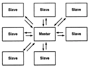
Figure 3.2: Master/Slave architecture. 33

Figure 3.3: Flowchart of parallel algorithm. 35

Figure 3.4: Flowchart showing steps followed by master. 36

Figure 3.5: Flowchart showing steps followed by Slave. 37

Figure 4.1: Weibull Probability Density Distribution for data set for

consensus method with 100,000 iterations and 33 processors. 43

Figure 4.2: Weibull Probability Density Distribution for data set for

Figure 4.4: Runtimes for parallel algorithm for different number of iterations. 45

Figure 4.5: Decrease in runtime with increase in number of processors. 45

Figure 4.6: Efficiency diagram for parallel consensus algorithm. 46

Figure 4.7: Speedup diagram for parallel consensus algorithm. 47

Figure 4.8: Accuracy of Consensus Results (100 iteration) of parallel

consensus method with different number of processors. 48

Figure 4.9: Accuracy of Consensus Results (1000 iterations) o f parallel

consensus method with different number o f processors. 49

Figure 4.10: Accuracy of Consensus Results (10,000 iterations) of parallel

consensus method with different number of processors. 49

Figure 4.11: Runtimes for parallel enhanced algorithm with different processors. 51

Figure 4.12: Efficiency diagram for parallel enhanced consensus algorithm. 52

Figure 4.13: Speedup diagram for parallel enhanced consensus algorithm. 52

Figure 4.14: Enhance consensus results for variation 4a

(Iterations 1000 & Consreps 1000). 54

Figure 4.15: Enhance consensus results for variation 4a

Haplotype Inference

1.1 O v erv iew

Humans have always been interested in gaining a better understanding of themselves and

their environment, to satisfy their curiosity, to survive, evolve and most of all to alleviate

suffering associated with human disease and improve living conditions.

Scholars have always been aware of differences in human race. Although, members

of the same species, millions o f human before us and billions alive today, are

phenotypically and genetically quite diverse. A quick glance around at people belonging

to different races and nationality gives us an idea of the differences amongst us.

However, biologist before Charles Darwin argued that the essential nature of a

species does not vary too much from one generation to the next. Charles Darwin

contended that the members of any species can vary, and that the variations within a

species can be either advantageous or disadvantageous leading to differential selection

and eventually contributes to the ongoing process of evolution [Jones 02].

Although Charles Darwin a British naturalist and Gregor Mendal called father of

are passed on to the members of the next generations within the same species was not

known, until the rediscovery of Mendel’s work by Hugo de Vries and Carl Correns in the

early 1900s. Mendel described the fundamental principles at the core of genetic

inheritance and demonstrates that the inheritance of traits follows particular laws.

According to Mendelian laws, physical characteristics are the result of the interaction of

genes contributed by each parent, which make up the characteristics of the offspring.

Mendel’s work provided a genotypic understanding of heredity, missing in earlier studies

focused on phenotypic approaches. Then, later in the 1930s and 1940s, the combined

understanding of Mendelism and Darwinism culminated in the “modem synthesis of

evolution” and formed the basis for modem genetics [Mayr 91].

1.1.1 Genetic M aterial

Although, the similarities between the theoretical behaviour of Mendel's particles, and the

visible behaviour of the newly discovered chromosomes, convinced scientists that

chromosomes carry genetic information. However, it was uncertain which component of

chromosomes either DNA or protein carried the hereditary information. It was not until

the late 1940s and early 1950s that DNA was identified and accepted as the chromosomal

component that carried hereditary information. Later, in 1953, Watson & Crick

discovered the structure of DNA [Shermer 06].

1.1.2 Structure & Organization o f Genetic M aterial

Human bodies consist of close to 50 to 100 trillion cells, organized into tissues such as

skin, muscle, and bone. As shown in Figure 1.1, each cell contains all of the organism's

genetic instructions, which are stored as DNA. DNA molecule is tightly wound and

packaged as a chrom osom e. Humans have two sets o f 23 chrom osom es in each cell. One

set inherited from each parent, a human cell; therefore, contains 46 of these chromosomal

THE STRUCTURE OF ONR Chromosome

btlhidtvm

teMttKNM

Hydrogtn bonds

Figure 1.1: Structure and organization of genetic materials in human cell [Jelinek 82]. Each DNA molecule that forms a chromosome can be viewed as a set of short DNA

sequences, know as genes. A set o f human chromosomes contains one copy of each of

the roughly estimated 30,000 genes in the human genome. A haplotype consist of all

alleles, one from each locus that is on the same chromosomes. To explain this concept, a

structure of a pair of chromosomes from mathematical point of view is further depicted in

Figure 1.2.

Genotype

I

2 2

2 1

1 2

1 1

2 2

Paternal Maternal

Components of a DNA molecule

1. DNA is a polymer made up of monomer units called nucleotides.

2. Each nucleotide consists of 5-carbon sugar (deoxyribose), a nitrogen-containing base

attached to the sugar, and a phosphate group.

3. There are four different types of nucleotides found in a DNA molecule. Each

nucleotides is representable by the following:

A: adenine (a purine)

G: guanine (a purine)

C: cytosine (a pyrimidine)

T: thymine (a pyrimidine)

The number of purine bases equals the number of pyrimidine bases. The structure of

the DNA molecule is helical, which contains equal numbers o f purines and pyrimidine

bases that are piled on top of each other, is depicted in Figure 1.3.

Hydrogens rxSrtfjK

Natiftgfkte I

DNA

Molecule:

Two

Views

Cyt9Sto8 9fl<J Thymift*

Bases -—■ litir \

fhocpbate 9 group <g>

1.1.3 Analysis o f Genetic M aterial

Watson and Crick’s discovery of the structure of DNA has facilitated the development of

genetic material analysis at a molecular level. Currently, DNA analysis is fast and

accurate. This is due to powerful new techniques and technological advances.

Now that the Human Genome Project (HGP) is almost complete, the next task is to

organize, analyze and interpret the massive amount of data from sequencing projects

throughout the world; and to perceive genetic differences as the basis of the wide range

of human traits.

1.1.4 Genetic Variation

The ultimate cause of genetic variation is the differences in the DNA sequences. Unlike

other species that predate humans by 150,000 years, humans have not had much time to

accumulate genetic variations. Approximately 99% of genetic information of humans is

identical, as confirmed by the completion o f the HGP. The HGP information was

completed in 2003 with the sequencing of 99% of the genome with 99.99% accuracy

[Francis 03].

Despite so many shared characteristics, the 1% difference is the cause of a wide range

of the phenotypic differences in human traits. The human genome comprises of about 3

billion base pairs of DNA. The level of human genetic variation is such that no two

humans, except for identical twins, have ever been, or will be, genetically identical.

Most of genetic variations do not affect how individuals function. However, some

genetic variations are related to disease, or the ability to survive changes in the

environment. Genetic variation; therefore, is the foundation of evolution by natural

selection.

Genomes are considered to be a collection of long strings, or sequences, from the

alphabet {A, C, G, and T}. Each element of the alphabet encodes one o f four possible

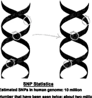
nucleotides, presented in Section 1.1.2 [Halldorsson 04]. Single Nucleotide

the genome sequence (see Figure 1.4), are the most common and smallest evolutionarily

stable variations of the human genome [Beaumont 04], [Chakravarti 98].

Figure 1.4: SNPs observed between chromosomes in DNA.

1.1.5 Single Nucleotide Polym orphism s (SNPs)

A Single Nucleotide Polymorphism (SNP) is a single base pair in genomic DNA at

which different nucleotide variants subsist in some populations; each variant is called an

allele [Lin 97], [Stephens 00]. For instance, an SNP can change the DNA sequence

AAGGCTAA to ATGGCTAA. In Figure 1.5, a more simplistic example o f chromosome

with three SNP sites is given. The individual is heterozygous at SNPs 1 and 3 and

homozygous at SNP 2. The haplotype are CCA and GCT.

Chrom. C, parental: ataggtccCtatttccaggcgcCgtatacttcgacgggaActata

Chrom, C, maternal: ataggtccGtatttccaggcgcCgtatacttcgacgggaTctata

Haplotype 1 -» C C A

Haplotype 2 -» <3 C T

Even though more than two alleles are not uncommon. In humans, SNPs are usually

biallelic; that is, there are two variants at the SNP site. The most common variant is

referred to as a major allele, and the less common variant is called a minor allele. SNPs

are differentiated from other mutations by a frequency of more than 1% in the population

[Orzack 03], [Peer 03].

SNPs are composed of about 90% of human genetic variations, and occur at 100 to

300 bases along the 3-billion-base human genome. Other types o f polymorphisms,

including, differences in copy number, insertions, deletions, duplications, and

rearrangements, are less frequent.

Two of every three SNPs involve the substitution o f C for T, and can occur in the

coding (gene) and non-coding regions of the genome. Although, many SNPs have no

effect on cell function, they can predispose people to a certain disease or influence their

response to a drug. SNPs constitute the genetic aspect of human response to

environmental stimuli such as bacteria, viruses, toxins, chemicals, and drugs. SNPs are

extremely valuable for biomedical, pharmaceutical research and medical diagnostics

[Rizzi 02]. An important characteristic of SNPs is that they are stable from one

generation to the next, which come in handy for tracking them in population studies.

SNP maps are being created by the joint efforts of HGP and SNP consortium,

consisting of a large number of pharmaceutical companies. So that additional markers

can be found along the human genome, which will make it much easier to navigate the

very large genome map created by scientist in HGP [Jorde 01].

1.1.6 Haplotypes

Although SNPs help to identify multiple genes, related with complex diseases such as

cancer, and diabetes [Lippert 02], [Niu 04a]. SNPs have provided researcher with even

more powerful tool, called “H aplotypes” [Clark 90].

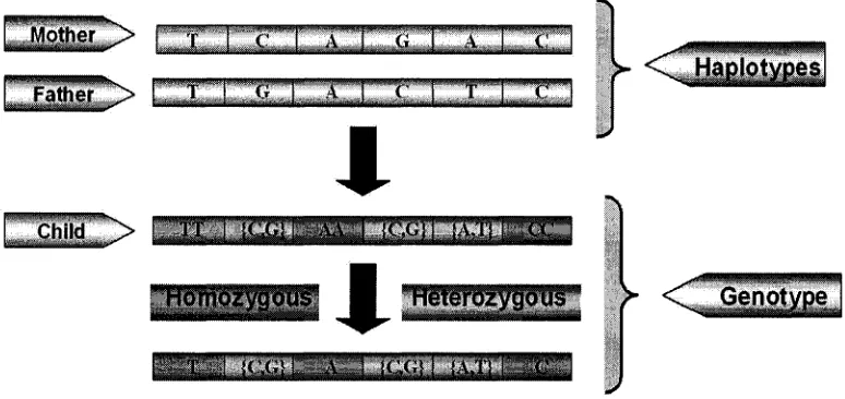
Haplotypes are the sets of SNPs along the human genome or chromosomes that are

most likely to be inherited generation after generation without recombination [Lam 00].

chromosome that are inherited as a unit [Lin 02], As a result, an individual possesses two

haplotypes, representing the maternal and paternal chromosomes for a given segment of

the genome [Bonizzoni 03], [Halldorsson 03]. Therefore, it can be stated that each copy

of the chromosome is called a haplotype. The conflation of the two inherited haplotypes,

which may be identical, is called a genotype. The difference in both haplotypes and

genotypes are elaborated below in Figure 1.6.

□ & £ L >

i_; -t-

1

l...a.

r:ig

I—f j g g b . I it . .[ :.c i T

I

'j

'."H o W fy g o u ^

35

Heterozygous

! i \ ti

< T. HaolotvDesI

Genotype

Figure 1.6: Difference between haplotypes and genotypes.

Only a small number of haplotypes are found in human. For example, as shown in

Figure 1.7, in any given population, the distribution of different haplotypes can be 55%,

30% and 8%. The other haplotypes are a variety of less common haplotypes [Gusfield

04].

..A..C..A..T..G.. T«. 55%

..A..C..C..G..C.. T.. 30%

A„ 08%

Several Others

12%

1.1.7 Significance o f Haplotypes

Complex diseases such as diabetes, cancer, heart disease, stroke, depression, or asthma

are affected by more than one gene. As a result haplotype data have been proven to be

much more informative than genotype data. Haplotype analysis can help researchers in

the following ways.

• To pinpoint the disease-causing locus, by observing the recombination events in

both family-based and population-based studies [Johnson 01].

• To identify the genetic variants that contribute to longevity and resist disease,

leading to new therapies with widespread benefits.

• To discover the genetic variants, involved in the disease and individual responses,

to therapeutic agents.

• To uncover the origin o f illnesses and discover new ways to prevent, diagnose,

and treat such illnesses.

• To customize medical treatments, based on a patient’s genetic make-up, to

maximize effectiveness and minimize side effects.

Also haplotypes are considered to be “molecular fossils”, because the frequency of a

certain haplotype in the sample can be used to infer its topological position in a

cladogram, providing snapshots of human evolutionary history [Niu 04b],

1.2 H a p lo ty p e In feren ce

The haplotyping problem for an individual is to determine a pair of haplotypes for each

copy of a given chromosome [Rizzi 02], [Wang 03].

Currently practical laboratory techniques provide un-phased genotype information for

diploids, that is, an unordered pair o f alleles for each marker. The reconstruction of

Unless an organism is a homozygote, its genotype might not uniquely define its

haplotype. A direct sequencing of genomic DNA from diploid individuals leads to

ambiguities on sequencing gels. This results in more than one mismatching site in the

sequences of the two orthologous copies of a gene (see Figure 1.8). These ambiguities

cannot be resolved from a single sample without resorting to other experimental methods.

A

M

"T G

C

1

2

3

4

5

6

A A T G T C

AG/A T G T / A G

A A T G A G

A G T G T C

(a) (b) (C)

Figure 1.8: An example of 6 SNPs with two homologues of an individual (a)

Individual’s haplotypes, (b) individual genotype, (c) another potential haplotype pair.

Although the acquisition of sequences of multiple alleles from natural populations

provides the ultimate description of genetic variation in a population, the time and labor

involved in obtaining the sequence data has limited the number of such studies. Any

means of acquiring the sequence data from population samples that decreases this effort

is pivotal to further achievements.

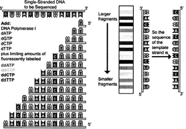
1.2.2 Biological M ethods for H aplotype Inference

The haplotype determination of several markers for a diploid cell is difficult. Unless the

individual is homozygous or haploid DNA is being sequenced existing genotyping

techniques cannot determine the phases of several different markers. For example as

shown in Figure 1.9, a genomic region with three heterozygous markers can yield eight

possible haplotypes. This uncertainty can, in some cases, be solved if pedigree genotypes

are available. However, even for a haplotype of only three markers: the genotypes of

father, mother, and offspring trios can fail to predict offspring haplotypes as much as 24%

A d d :

DNA P©lyWM»«i f dATP

d G T P dC T P dTTP

p b s bmittng a m o u n t* o f fUiorwKsenfly la tw id d ddAT (*

ddCTP ddTTP

i t

111

,

B m m m

i i i i i i

M a n a a f t * *

S' 'tmgm? fragments swatter fragments 31

m »£»w0«» m

of the temptate g | strand * Z .

3’

Figure 1.9: Sequencing example of a single stranded DNA.

An example is shown below in Table 1.1. Consider two loci on the same

chromosome. Each locus has two possible alleles; the first locus is either, A, or a, and

the second locus being B or b. If the organism's genotype is AaBb, there are two possible

sets of haplotypes, corresponding to which pairs occur on the same chromosome:

Table 1.1: Example of two possible sets of haplotypes.

Set Haplotype at chromosome 1 Haplotype at chromosome 2

Haplotype set 1 AB ab

Haplotype set 2 Ab aB

In this case, more information is required to determine which particular set of

Alternatively, several direct molecular haplotyping methods have been developed for

haplotype inference. The methods are based on the physical separation of two

homologous genomic DNAs before genotyping can be used. Examples include the

following:

1. M l-PCR Method

2. DNA cloning somatic cell hybrid construction

3. Single molecule dilution

4. Allele-specific, single-molecule, and long-range PCR

1.2.3 Significance and Shortcomings o f M olecular H aplotyping M ethods Significance

1. Typically, these approaches are largely independent of pedigree information

[Ding 03], [Niu 04b], [Ruano 90], [Tost 02].

2. Molecular haplotyping techniques, such as the M l-PCR method, have resulted in

a genotyping success rate, for single copy DNA molecules, of approximately

100%.

Shortcomings

1. Typically, molecular haplotyping methods are time consuming and labor

intensive.

2. Some of these methods, including for instance the allele-specific and single­

1.2.4 Com putational M ethods

The advent of the polymerase chain reaction (PCR) [Saiki 85], [Scharf 86] has

substantially accelerated the process of genomic DNA to sequence data by eliminating

the cloning step. The direct sequencing of PCR products works well for mtDNA or for

DNA from isogenic, or otherwise homozygous or hemizygous regions, but

heterozygosity in diploids results in an amplification of both alleles.

By using asymmetric amplification, with unequal concentrations of the two primers,

single-stranded DNA products can be directly sequenced. In a heterozygote, an

asymmetric PCR results in amplification products of both homologues. The resulting

superimposition of the two sequencing ladders for the two alleles produces a vast number

of possible haplotypes for any heterozygous individual. If there are n such “ambiguous”

sites in an individual, then there are 2n” possible haplotypes. The challenge is to devise a

scheme, whereby haplotypes can be inferred from a series of these ambiguous sequences,

constructed from samples of diploid natural populations.

Input to the computational method consists primarily of n genotype vectors, each with

length m, where each value in the vector is 0, 1, or 2. Each position in the vector

represents an SNP on the chromosome. The position in the genotype vector has a value of

0 or 1 for homozygous site, and a value of 2, otherwise, for a heterozygous site [Lippert

02], [Niu 04a].

Given an input set of n genotype vectors, the computational methods are used to

calculate an optimal solution to the Haplotype Inference (HI) problem that is to determine

the best possible haplotype pairs, which provide complete SNP fingerprint information

for that chromosome, and for each individual in a sample data set [Lancia 01], [Li 04].

1.2.5 Significance and Shortcom ings o f Computational M ethods

Although haplotypes can be directly determined by biological methods, an experimental

study of haplotypes is technically difficult, because the direct molecular haplotyping

H ow ever, com putational m ethods, although not perfectly accurate, are cost efficient

and less laborious than that of biological methods, providing a more practical and

accurate alternative to experimental haplotyping methods [Adkins 04].

1.3 D ifferen t A lg o rith m ic A p p ro a ch es

Haplotypes are much more informative and helpful than SNPs, since they capture linkage

disequilibrium information far better than SNPs alone [Casey 03], [Clark 04], [Service

99]. Consequently, haplotype inference is important for many genetic studies, including

related studies for complex diseases that are related a particular phenotype in a specific

genetic region.

There are different approaches to solve this problem, including the nuclear family

design, in which the haplotypes are inferred from the parent’s genotypes of the

individual. However this involves a substantial increase in genotyping costs. Also, it is

difficult to recruit the parents of the diseased individuals, since most of the complex

diseases are late onset. As a result, it is much easier to genotype individuals for complex

diseases by a case-control design rather than a family-based design.

The computational methods for the haplotype reconstruction problem can be

categorized as follows:

Haplotype Inference Using Population Data 1. Combinatorial Methods

a. Rule-Based Methods, e.g., Clark’s Inference Rule.

b. Coalescent Models

Markov-chain Monte Carlo (MCMC) Method

(e.g., Pseudo-Gibbs Sampler (PGS) Algorithm)

2. Statistical Methods

a. M axim um Likelihood Approach, e.g., Expectation m axim ization algorithm.

b. Bayesian Inference Methods, e.g., Partition Ligation (Haplotyper, Phase.)

1.3.1 Rule based Methods Clark’s Rule

Clark introduced the earliest algorithm for haplotype reconstruction, and the inference of

haplotype frequencies from genotype data, based on the principle of maximum parsimony

[Clark 90],

The algorithm, known as Clark’s Rule is used to assign the smallest number of

haplotypes to the observed genotype data. First, the algorithm forms an initial set of all

the unambiguous haplotypes that include all the homozygotes and single-site

heterozygotes. This is the set of resolved haplotypes. The algorithm is then applied to

determine the remaining haplotypes, based on the set of unambiguous haplotypes that is,

Clark’s Rule is used to determine if any of the ambiguous haplotypes can be explained

according to the recently resolved haplotypes. Each time that a new haplotype is

identified, it is added to the set of resolved haplotypes, until all the genotypes are

resolved or cannot be explained by the resolved haplotypes.

For this algorithm, it is assumed that the input genotype data contains unambiguous

homozygous haplotypes, a necessary condition for starting the algorithm. According to

Clark, when all the haplotypes are determined, based on the principle of maximum

parsimony, the solution is unique and accurate [Clark 90]. Compared with the results

obtained by experimental methods, the results generated by application o f Clark’s

algorithm to certain empirical data is found to be reliable.

The algorithm does not assume HW equilibrium, unlike the other procedures for

haplotype reconstruction; however, the departure from the HW equilibrium, by

modification of Clark’s algorithm Gusfield redefined it as the “ Maximum Resolution”

(MR) problem [Gusfield 00], [Gusfield 01], The MR problem can be stated as follows:

“Given a set of both ambiguous and unambiguous vectors, which is the maximum

number o f ambiguous vectors that can be resolved by successive iterations of Clark’s

inference rule”.

The MR problem has proved to be NP-hard and Max-SNP-complete by Gusfield. He

has also proposed a solution by first reformulating the problem as a directed graph

problem and then solving the graph problem with integer linear programming [Gusfield

01], [Gusfield 03]. Despite the Clark’s algorithm’s simple nature, it is quite popular due

to its relatively straightforward procedure, and capability to handle a large number of

loci, when the haplotype diversity is rather limited in the population.

Clark’s algorithm does exhibit some limitations. For instance, the algorithm might not

even run, when there are no unambiguous haplotypes (i.e., either homozygotes or single­

site heterozygotes) in the population genotype data. Also, since the results depend on the

order of entry of ambiguous haplotypes the algorithm does not give unique solutions;

thus, Clark’s algorithm might not be able to resolve many haplotypes, where there are a

greater number of distinct haplotypes, due to recombination o f the hotspots, in a

relatively small sample size. Although Clark’s algorithm does not explicitly assume the

Hardy-Weinberg equilibrium (HWE), the performance is still relatively sensitive to the

deviation from the HWE [Niu 02],

1.3.2 Coalescent M odels

The coalescent-based model is assumed to represent the evolutionary history by a rooted

tree, where each leaf of the tree represents each given sequence [Gusfield 91]. The model

also yields, at most, one mutation per given site in the tree, infinite site model, restricting

the repeated mutations, and thus supporting no recombination assumption. As a result,

Pseudo-Gibbs Sampler (PGS) Algorithm

The coalescence based Markov-chain Monte Carlo (MCMC) approach has been proposed

for haplotype reconstruction from genotypic data [Liu 01], [Stephens 01]. The PGS has

been developed by using Gibbs sampling algorithm to calculate the approximate sample

from posterior distribution [Stephens 01],

Also, the PGS algorithm has been modified to use a modified version of the partition

ligation approach allows the recombination and decay of linkage-disequilibrium with

distance [Niu 02], The advantages o f PGS include the incorporation o f the coalescence

theory into its prior and a reliable performance. Conceptually, the Gibbs sampler

alternates between two coupled stages.

However, the PGS algorithm lacks the overall “goodness” o f the constructed

haplotypes, since the algorithm is not a full Bayesian model. Also, PGS’s piece-by-piece

strategy to update the haplotypes, based on the existing haplotypes is slow and requires a

tremendous number of iterations in the range of millions for an accurate result generation.

[Stephens 03],

Perfect and Imperfect Phylogeny (PPH)

The perfect phylogeny haplotype problem can be defined as follows:

Given a set of genotypes, find a set of explaining haplotypes, which defines an un-rooted

perfect phylogeny. The perfect phylogeny problem assumes “no recombination”, as well

as the infinite site model [Bafna 02], [Bafna 03]. The problem has been proven to be NP-

hard [Kimmel 04], A phylogeny-based algorithm is adopted to deterministically infer

haplotypes, according to phylogenetic reconstruction [Chung 03b], [Eskin 04a], [Gusfield

02

],

The program, “ Perfect Phylogeny Haplotyper” has been developed for determining

if the input un-phased genotype data can be explained by haplotype pairs evolved on

perfect phylogeny [Chung 03 a]. The PPH program solves a problem by first reducing it

problem [Barzuza 04], [Daly 01], [Gusfield 02]. The program is fast, verifies its results,

and also provides a corresponding tree format for the solution [Halperin 04b].

Recently, a new method has been developed realized by using imperfect phylogeny

that extends the framework of PPH by allowing for recurrent mutations and

recombinations [Halperin 04a]. The method partitions the multiple linked SNPs into

blocks, and for each block, predicts an individual’s haplotype. The haplotype blocks are

then assembled to form a long-range haplotype by utilizing the PL idea [Niu 02]. The

imperfect phylogeny method appears to be more reliable than PPH, and allows for the

handling of missing data and for resolving a large number of SNPs.

1.3.3 Expectation-Maximization (EM) Algorithm

The expectation-maximization (EM) algorithm was first introduced, by Dempster et al. in

1977 [Dempster 77]. They have formalized the use of the EM algorithm for a haplotype

frequency estimation that maximizes the sample probability.

Excoffier and Slatkin [Excoffier 95] were the first to discuss the use o f the EM

algorithm for estimating the population haplotype probabilities, based on the maximum

likelihood, and finding the haplotype probability values that optimize the probability of

the observed data, based on the assumption of HWE. They authors have demonstrated

how the EM algorithm can be extended to apply to a genetic sequence and highly

variable loci data [Excofier 95],

Under the assumption of the HWE, the EM algorithm is an iterative method for

computing successive sets of haplotype frequencies. The iterative step can be represented

as follows:

9a(k+1) = E0(k)(na|G )/2n, (1.1)

where 0 ® is the present estimate o f the haplotype frequencies, and na is the count o f

haplotype ‘a’ in G.

The EM algorithm is based on the solid statistical theory, and performs well for the

[Excofier 95], [Fallin 00]. Although the algorithm makes an explicit assumption of HWE,

its performance in simulation studies is not much affected by the departures from HWE,

especially increased homozygosity [Niu 02],

The limitations of the EM algorithm include its sensitivity to the initial values of

haplotype frequencies. Also it is well known that the EM algorithm can be trapped in a

local mode, if there exist a local maxima, leading to locally optimal maximum likelihood

estimates (MLEs). The local mode problem increases with the increasing number of

distinct haplotypes. It is noteworthy that the initial values of the haplotype frequencies

are reasonably close to the true population frequencies and help [Excofier 95], [Kelly 04],

In addition, the standard EM algorithm is limited in its capability of handling a large

number of loci [Eskin 04b].

1.3.4 Partition Ligation (PL) Algorithm

The Partition-ligation (PL) algorithm, a divide-conquer-combine approach has been

introduced to handle a large number of loci. [Niu 02]. The PL algorithm depends on the

assumption that a long-range haplotype is a combinatorial set of atomistic units,

supported by the empirical observations of the underlying haplotype block patterns of the

human genome [Daly 01].

First, he long-range haplotype is partitioned into a series of smaller, atomistic units.

As a result, the haplotype phasing for each atomistic unit becomes tractable, and the long-

range haplotype is considered the ligated product of these units. In the ligation step, one

of two strategies can be adopted: hierarchical ligation or progressive ligation [Niu 02].

HAPLOTYPER and PLEM PL developed are realized by hierarchical ligation; whereas,

the variants of the progressive ligation were implemented by a modified version of

PHASE version 1.0 and SNPHAP [Niu 02], [Qin 02].

The algorithm, implemented in HAPLOTYPER, is based on a new Monte Carlo

approach, a robust Bayesian procedure with the same statistical model as the EM. The

new algorithm has been designed to overcome the shortcomings of the existing, and

iterative-sampling algorithms. The method uses two novel techniques PL and prior

annealing to divide the haplotypes into smaller segments, and Gibbs sampler for partial

haplotype construction and segment assembly. The method can handle HWE violations,

missing data, and recombination hotspot occurrences [Niu 02].

1.3.5 Haplotype Inference using Pedigree Data

Pedigree data differs from population data in the relations that exist among the genotyped

individuals, which otherwise, are considered to be independent in population-based

studies. For pedigree data, the relations of the parenthood are related individuals [Li 03a].

A number of linkage analysis programs are used to reconstruct the haplotypes, by

using pedigree data. These include Genehunter, Simwalk2, and Merlin [Sobel 96]. Here,

it is assumed that the linked markers are in linkage equilibrium, implying that all possible

haplotype configurations have same likelihood in the case of phase ambiguity [Schaid

02], For Genehunter, the results depend on the order in which the alleles are entered.

Consequently, for the few haplotype ambiguities, Genehunter, Merlin, and Simwalk2,

should be applied. The use of trios is becoming more and more popular due to their

relative efficiency and ease of sample collection.

The Rule-based method, along with the genetic algorithm, has also been proposed for

haplotype inference from pedigree genotype data. Implemented in HAPLOPED, the

algorithm has shown potential, but cannot be compared to the existing programs such as

GENHUNTER and SIMWALK due to the differences in assumptions and data

requirements [Tapadar 00].

EM-based haplotype inference methods have been developed without the assumption

of linkage equilibrium among the linked markers. The nuclear family data have been

shown to be more efficient than that of the Lander-Green algorithm o f Genehunter

[Rhode 01].

A rule-based “ minimum- recombinant haplotyping” (MRH) algorithm exhaustively

searches for all possible minimum-recombinant haplotype configurations in large

be imputed from identity-by-descent alleles [Doi 03], [Orzack 03]. Although trios are

more suitable to sample than large pedigrees, for certain complex traits with the late onset

of a disease, the parental DNA samples often cannot be typed.

1.3.6 Haplotype Inference using Pooled DNA Samples

To reduce the high cost of genotyping, pooled DNA samples have been introduced. An

allele-specific, long-range PCR method for the direct measurement of haplotype

frequencies in DNA pools has been devised [Istrail 97]. This method, however, is not

feasible for neighboring SNPs that are separated by intervals longer than 420 kb.

Pooling complicates the haplotype configurations and adds to the ambiguities in the

haplotype frequency estimation. Although DNA pooling is very cost-efficient, it can

increase errors in allele and haplotype frequency estimations [Yang 03], Instead, the use

of small DNA pools, for instance, a pool size of 2, has been proven to be superior to the

use o f large pools [Hoh 03], [Wang 03].

Two EM-based algorithms have been developed for haplotype reconstruction from

the pooled genotype data. An EM algorithm for obtaining the maximum likelihood

estimations (MLEs) and the haplotype frequency estimations has been developed, to cope

with the missing data [Yang 03].

1.4 Organization of Thesis

This thesis is organized in 5 chapters. Chapter-2 gives an overview of the previous

research in the related area and discusses different approaches. In chapter-3 we presented

the proposed methodology for an efficient parallel algorithm for haplotype inference

based on rule based approach and consensus methods. In chapter-4 we discuss the results

based on the proposed approach. The analysis in this chapter measures the performance

of parallel algorithm. Chapter-5 includes conclusion and suggests directions for future

Review on Clark’s Algorithm

2.1 Introduction to Clark’s Algorithm

In 1990s, A. G. Clark first introduces the Clark’s Algorithm. It continues to be a popular

method for solving the haplotype inference problem. Clark’s algorithm consist of the

following four steps:

1. The identification of initial resolved haplotypes: these are retrieved from the

genotype vectors with either no ambiguous sites or a single ambiguous site, since

these genotypes can be resolved only in one way.

2. Resolution of the ambiguous genotypes: here, there is more than one ambiguous

site. It requires the help of the initial resolved genotypes and Clark’s Inference

Rule. Clark’s Inference Rule is stated as follows:

Suppose A is an ambiguous vector with h ambiguous sites, and R is a resolved vector

that is a haplotype in one of the 2 h -l potential resolutions of vector A. Then, infer that A

resolved vector NR. All the resolved positions of A are set the same in NR, and all of the

ambiguous positions in A are set in NR opposite to the entry in R. Once inferred, vector

NR is added to the set of the known resolved vectors, and vector A is added to the set of

ambiguous vectors.

3. To resolve vector R can be used to resolve an ambiguous vector A if and only if

vector A and vector R consist of identical unambiguous sites.

4. Clark’s inference rule is repeatedly applied until either all the genotypes have

been resolved or no further genotypes can be resolved.

Clark’s algorithm appears to be straightforward and should work in theory. However,

following situations are problematic:

1. The sample data do not contain any homozygotes or heterozygotes; therefore, the

algorithm cannot be run.

2. All the genotypes are not resolved by the end of the inference method.

3. The haplotypes can be erroneously inferred, if the crossover product of two real

haplotypes is identical to that of another actual haplotype.

4. It is possible that these problems depend on the average heterozygosity, the length

of the genomic sequence, sample size, and the recombination rates of the sites.

The basis of the method is that a phase-ambiguous sampled genotype data is likely to

contain known common haplotypes.

2.2 Genetic M odel of Clark’s Algorithm

Clark’s algorithm assumes that the sample is small, compared to the actual population

of the current population and that the sampled individuals are randomly drawn from the

population. Thus, the initial resolved haplotypes represent common haplotypes, occurring

with a high frequency in population.

Also, Clark’s method is used to resolve the identical genotypes in the same way,

assuming that the history leading to the two identical genotypes is identical. This is

justified by the “infinite sites” model of population genetics, in which only one mutation

at a given site has occurred in the history of the sampled sequences [70].

The previous assumptions are consistent with the way Clark’s algorithm gives

preference to resolutions, involving two initially resolved haplotypes. The application of

the Inference Rule is justified as long as the result is the accurate resolution of a

previously ambiguous genotype. Similarly, the rule gives preference to resolutions,

involving one originally resolved haplotype, compared with involving no initially

resolved haplotypes.

The “distance” of an inferred haplotype NR from the initial resolved vectors can be

defined as the number of inferences used on the shortest path o f inferences from some

initial resolved vector, to vector NR. Such rationalization of Clark’s algorithm becomes

weaker, since it is used to infer the vectors with the increasing distance from the initial

resolved vectors. However, Clark’s Inference Rule is justified in [14] by the empirical

observation of the aforementioned consistency.

2.3 Effect o f Different Implementation Specifications on Clark’s

Algorithm

The implementation of the Inference Rule results in many options regarding vector R: the

initial resolved vector, for any ambiguous vector, and any one choice, can result in a

different set of future choices. Consequently, one succession of the choices might resolve

in all the ambiguous vectors in one way; whereas, another implementation, involving

different choices might resolve the vectors in a different way, or result in orphans

For example, consider two resolved vectors 0000 and 1000, and two ambiguous

vectors 2200 and 1122. Vector 0000 is used to resolve vector 2200, creating the new

resolved vector 1100, which is then used to resolve 1122. In this way, both of the

ambiguous vectors are resolved; that is, the result is the resolved vector set 0000, 1000,

1100, and 1111. But, 2200 can also be resolved by applying 1000, resulting in resolved

vector 0100. However in this case, none of the three resolved vectors, 0000, 1000, or

0100 can be further used to resolve the orphan vector 1122.

The results generated by Clark’s method depend on the order of the data set. As a

result, Clark suggests a reordering of the data multiple times, and running the algorithm

on each reordered data set. The “best” solution among these executions is then selected.

In regards to the best solution, Clark reports that the solution with the highest number

of resolved genotypes; that is, a lower number of orphans, should be preferred, since the

results indicate that the inference method tended to produce incorrect vectors only when

the execution also leaves orphans. This implies that if the early ambiguous genotypes are

inferred, incorrectly, by the inference rule, it will render the method, unable to move

further and resolve the remaining genotypes [Clark 90].

2.4 Clark’s Algorithm and Maximum Resolution Problem

According to Clark, a complete haplotype resolution, based on maximum parsimony,

results in a solution that is more likely to be correct and unique. This is depicted by the

results obtained by the implementation of Clark’s algorithm on certain empirical data.

The method is proved to be reliable by comparing the results with those of the

haplotypes, obtained from direct molecular methods.

This has led to a reformulation of Clark’s algorithm by Gusfield as a “maximum

resolution” (MR) problem. The MR problem is stated as follows:

Given a set of both homozygous and heterozygous genotypes, what is the maximum

number of ambiguous genotypes that can be resolved by successive applications of

The MR problem requires that Clark’s algorithm be implemented in such a way that

the consequences of the earlier choices of the inference rule on the later applications of

the inference rule can be weighed. Gusfield has demonstrated that the MR problem is

NP-hard, and Max-SNP complete. He reformulated the MR problem as a problem on

directed graphs. An exponential time reduction to a graph theoretic problem can be

solved by using integer linear programming.

An acyclic graph is used to represent all the possibilities, resulting from the

implementation of Clark’s algorithm, where each node represents a haplotype resolution

in some implementation of Clark’s inference rule. Nodes u and v are connected by an

edge, only if this haplotype resolution can be used to resolve an ambiguous genotype in

the sample data, resulting in the inference of the haplotype at node v.

Gusfield has also showed that the MR problem can thus be formulated as a search

problem on this graph, and can be solved by using integer linear programming.

Gusfield’s results indicate that this approach is very efficient in practice, and that linear

programming alone is sufficient to solve the maximum resolution problem. However, the

results also indicate that the solution of the MR problem is not an entirely suitable way to

find the most accurate solutions. One major problem is that there are often many

solutions to the MR problem, that is, many ways to resolve all of the genotypes.

Moreover, since Clark’s method should be run many times, generating many solutions, it

is not clear how to use the generated results. In fact, no published evaluation of Clark’s

method exists, except for the evaluation by [Liu 04]. He proposed an approach to this

issue. Almost all have run Clark’s method only once on any given data set. This ignores

the stochastic behaviour of the algorithm, and these evaluations are uninformative. The

critical issue in Clark’s method is how to understand and exploit its stochastic behaviour.

2.5 V a ria tio n s o f th e Im p lem en ta tio n o f C la r k ’s A lg o rith m

In Gusfield’s work, different variations of the implementation of Clark’s method have

been studied. These variations of the rule-based approach differed in how the list of

how the list of ambiguous genotypes is analyzed. These variations can differ, in the

genetic models with which they are consistent [Orzack 03].

They report the results of several variations of the rule-based method, including

Clark’s original method by using a set of 80 genotypes at the human APOE locus; of

these genotypes, 47 are ambiguous with 9 SNP sites in each genotype. Table 2.1 shows

the different variations they studied in [Gusfield 03]. They were designed the variations

in response to following basic questions:

■ Does the reference list also include inferred haplotypes in addition to the real

haplotypes or not?

■ Whether duplicate haplotypes are removed or retained in the reference list?

■ Whether the duplicate ambiguous genotypes are consolidated or not?

■ Is the reference list randomized?

Table 2.1: The characteristics of the eight rule-based algorithms for haplotype inferral.

Variation Duplicate haplotypes

Haplotype list randomized? Ambiguous genotypes consolidated? Preference for real haplotypes? Frequency preference Identical genotypes Real Inferred

1 Retained Retained Yes No No Population

May be resolved differently

2 Retained Retained Yes Yes No Population Resolved identically

2a Removed Retained Yes Yes No Weak Resolved

identically

2b Retained Retained No No Yes Population Resolved identically

2c Removed Retained No Yes Yes No Resolved

identically

3 Retained Retained No No No Strong

Maybe resolved differently

4a Removed Removed Yes Yes No No Resolved

identically

4 b R e m o v e d R e m o v e d N o Y e s Y e s N o Resolved

identically

The real haplotype pairs are experimentally inferred in order to evaluate the inferral

solutions. Each is capable of resolving all of the 47 ambiguous genotypes. The solutions

vary considerably with respect to accuracy. As a result, a solution, chosen at random

from the solutions, is probably not very accurate. Consequently, an important issue in

using rule-based methods, such as Clark’s method, is how to exploit the many different

solutions that it can produce.

2.6 Consensus Approach

The multiplicity of solutions demands an effort to understand how they can be used to

provide a single accurate solution. Gusfield has introduced the following strategy in

[Gusfield 03] to greatly improve the accuracy of any of the variations of the rule-based

method.

1. Run the algorithm repeatedly, each time randomizing the order of the input data.

Depending on the variation, the decisions made by the method are also

randomized. The result is a set of solutions that might be quite different than

another.

2. Tally the different inferrals for any given genotype across the results of all the

repetitions for the given sample data. In these runs, record the haplotype pair that

was most commonly used to explain each genotype g. The set of such explaining

haplotype pairs is called the “full consensus” solution.

3. Or Select the runs that produce a solution using the fewest, or close to the fewest

number of distinct haplotypes. In those runs, record the haplotype pair that was

most commonly used to explain each genotype g. The set o f such explaining

haplotype pairs is called the “consensus” solution.

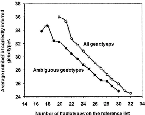
The consensus solution is reported to have a significantly higher accuracy than the

relationship between the numbers of haplotypes used in a solution and the correct number

of inferrals, as depicted in Figure 2.1 [Orzack 03].

36

-jfc </>

8 2L 32 ‘ 'S t

§ 30 -

2 o>

28 - Am biguous genotypes

o>

26

-24

14 16 18 20 22 24 26 28 30 32 34

N um ber o f haplotypes on the reference list

Figure 2.1: The relationship between the average number of correctly inferred haplotype

pairs and the number of reference haplotypes.

Also, it is reported that the solutions that uses the smallest and next-to-smallest

number of distinct haplotypes, the haplotype pairs used with higher frequency were

almost always correct. For instance, genotype resolutions reported above 85% o f the time

in results were correct in most cases. This provides an opportunity to home in on the

inferred haplotypes in results that can be used with confidence. Also, it can be used to

guide the experimental efforts for the detection of true haplotypes so as to minimize the

Proposed Methodology

This thesis presents two new and efficient parallel algorithms for Haplotype Inference

based on Consensus Method proposed by Orzack and Gusfield in [Orzack 03]. One

approach parallelizes the consensus method. Whereas the second parallel algorithm

introduces an improved variation of consensus method. The parallel algorithms are then

further used firstly to systematically investigate the affect of, number of iterations of

Clark’s Inference rule, on the number of accurately inferred genotypes, and secondly to

explore better ways to fish out the results, with higher accuracy, from among the many

results generated by numerous iterations of Clark Inference Rule.

The parallel algorithms were implemented using Message Passing Interface (MPI).

The code was developed in C++. The algorithms divide the computational tasks almost

equally among the number of nodes. The data set remains the same for each processor,

which assists in keeping the communication overhead to a minimum. Thus ensuring

maximum possible speed up, for optimal combination of number of iterations and

number of processors.

The sequential algorithm used as basis for the parallel algorithms is based on Clark’s

3.1 The Sequential Algorithm

The sequential algorithm for consensus method closely follows Clark’s Inference rule,

and resembles variations 4a and 4b of Clark’s algorithm reported by Orzack. The

sequential algorithm however departs from variations 4a and b in that the duplicate

genotypes are not consolidated, and thus could be either resolved identically or

differently from each other.

The algorithm first reads in the input data, consisting of phase unknown ambiguous

genotypes. The input data is then processed to create a Difference Matrix, an array that

stores the number of site differences for each haplotype pair. The difference matrix is

then used to select the haplotype pairs with either none or one site difference i.e.

homozygotes or single site heterozygotes. These haplotype pairs are then used to generate

the Initial Reference List.

The Clark Inference Rule is then applied repeatedly for the specified number of times

to resolve the ambiguous genotypes and the results are integrated to generate the

Consensus Results.

The pseudo code for the sequential algorithm is given below. Also, the sequential

algorithm is depicted in Figure 3.1.

Algorithm:

Read input data

Generate difference matrix Generate reference list

Generate list o f ambiguous genotypes

While less than iterations

Randomize haplotype and ambiguous genotypes lists (only fo r variation 4a) Perform Clark’s Inference Rule

Yes No

Print Results

Finish If Final Iteration „

Main

Assemble Final Consensus

Results

Integrate Results for Consensus Read Input

Make Diff Matrix Make Reference List

Figure 3.1: Flowchart showing sequential algorithm process.

3.2 Parallel Algorithm For Consensus M ethod

3.2.1 Computational Task Distribution

As Consensus method is based on the stochastic behavior of the Clark’s algorithm, it

requires a large number of iterations of Clark’s algorithm. The new algorithm therefore

exploits the parallelism in Consensus method by dividing the required number of

iterations of Clark’s algorithm among the available nodes. Each node thus first performs