GENOMIC SELECTION
Is Structural Equation Modeling Advantageous for
the Genetic Improvement of Multiple Traits?
Bruno D. Valente,*,1Guilherme J. M. Rosa,*,†Daniel Gianola,*,†,‡Xiao-Lin Wu,‡and Kent Weigel‡
*Department of Animal Sciences,†Department of Biostatistics and Medical Informatics, and‡Department of Dairy Science, University of Wisconsin, Madison, Wisconsin 53706
ABSTRACTStructural equation models (SEMs) are multivariate specifications capable of conveying causal relationships among traits. Although these models offer insights into how phenotypic traits relate to each other, it is unclear whether and how they can improve multiple-trait selection. Here, we explored concepts involved in SEMs, seeking for benefits that could be brought to breeding programs, relative to the standard multitrait model (MTM) commonly used. Genetic effects pertaining to SEMs and MTMs have distinct meanings. In SEMs, they represent genetic effects acting directly on each trait, without mediation by other traits in the model; in MTMs they express overall genetic effects on each trait, equivalent to lumping together direct and indirect genetic effects discriminated by SEMs. However, in breeding programs the goal is selecting candidates that produce offspring with best phenotypes, regardless of how traits are causally associated, so overall additive genetic effects are the matter. Thus, no information is lost in standard settings by using MTM-based predictions, even if traits are indeed causally associated. Nonetheless, causal information allows predicting effects of external interventions. One may be interested in predictions for scenarios where interventions are performed,e.g., artificially defining the value of a trait, blocking causal associations, or modifying their magnitudes. We demonstrate that with information provided by SEMs, predictions for these scenarios are possible from data recorded under no interventions. Contrariwise, MTMs do not provide information for such predictions. As livestock and crop production involves interventions such as management practices, SEMs may be advantageous in many settings.
S
TRUCTURAL equation models (SEMs) (Wright 1921; Haavelmo 1943) are multivariate models that account for causal associations between variables. They were adap-ted to the quantitative genetics mixed-effects models set-tings by Gianola and Sorensen (2004). These models can be viewed as extensions of the standard multiple-trait models (MTMs) (Henderson and Quaas 1976) that are capable of expressing functional networks among traits. Gianola and Sorensen also investigated statistical consequences of causal associations between two traits when they are studied in terms of MTM parameters, expressed as functions of SEM parameters. Additionally, these authors developed inference techniques by providing likelihood functions and posterior distributions for Bayesian analysis and addressed identifi -ability issues inherent to structural equation modeling.The work of Gianola and Sorensen (2004) was followed by several applications of SEMs to different species and traits, such as dairy goats (de los Camposet al.2006a), dairy cattle (de los Campos et al. 2006b; Wuet al. 2007, 2008; Koniget al.2008; Heringstadet al.2009; Lopez de Maturana
et al. 2009, 2010; Jamrozik et al. 2010; Jamrozik and Schaeffer 2010), and swine (Varona et al. 2007; Ibanez-Escriche et al.2010). Extensions were proposed to account for heterogeneity of causal models (Wu et al.2007), to in-clude discrete phenotypes via a“threshold”SEM (Wuet al.
2008), to study heterogeneous causal models using mixtures (Wu et al. 2010), and to analyze longitudinal data using random regressions (Jamrozik et al. 2010; Jamrozik and Schaeffer 2010). The likelihood equivalence between MTMs and SEMs was addressed by Varonaet al. (2007). As an attempt to tackle the problem of causal structure selection, Valenteet al.(2010) proposed an approach that adapted the inductive causation (IC) algorithm (Verma and Pearl 1990; Pearl 2000) to mixed-models scenarios, allowing searching for recursive causal structures in the presence of confound-ing resultconfound-ing from additive genetic correlations between
Copyright © 2013 by the Genetics Society of America doi: 10.1534/genetics.113.151209
Manuscript received March 14, 2013; accepted for publication April 11, 2013
1Corresponding author: Department of Animal Sciences, 444 Animal Science Bldg.,
traits. The development and application of such methodol-ogies are reviewed in Wu et al. (2010) and Rosa et al.
(2011).
All aforementioned articles have applied Gianola and Sorensen’s (2004) mixed-effects SEM and inference machin-ery. However, the contrasting of the results from SEMs and MTMs were generally restricted to the usual model compar-ison criteria based on goodness of fit or by exploring the SEM’s greater flexibility in expressing complex associations among phenotypes (e.g., the possibility of distinguishing be-tween direct and indirect effects among traits). Nevertheless, some authors have pointed out that even though reduced SEMs and MTMs may yield similar inferences regarding dis-persion parameters, interpretation and use of the models for selection purposes could differ if causal effects among traits actually exist (de los Camposet al.2006b). Resolving this major issue would indicate how important or useful SEM could be for breeding programs.
Clearly, investigating whether and how selection would differ between a SEM and a MTM applied to a set of phe-notypic traits is of importance and interest. However, this has not been done yet. So far, almost all articles that fol-lowed Gianola and Sorensen (2004) had a similar structure. First, they proposed a specific application of a mixed-effects SEM to study a set of traits assumed to have complex rela-tionships among them, with the rationale that accounting for causal relationships might lead to a better model than the traditional MTM. Then, results in terms of inferences and causal interpretations for the structural coefficients among phenotypes were presented. Finally, they presented inference regarding the remaining parameters in terms of the “reduced”model. To do this, estimates of additive ge-netic effects and associated dispersion parameters pertain-ing to the SEM are “rescaled”in terms of those from the standard MTM to provide meaningful comparisons. While these articles focus on inferences of structural coefficients and their causal interpretations, fitting a SEM and convert-ing its genetic parameters to MTM parameters negates the advantages of using a causal model as a SEM for quantita-tive genetic analysis. Consequently, the application of the SEM loses its appeal, especially as this approach introduces additional complexities such as causal structure selection (Valente et al. 2010) and parameter identifiability issues (Wuet al.2010).
Many questions regarding the use of SEMs in the animal or plant breeding context include, for example, the follow-ing: (1) From a plant and animal breeding standpoint, why do we want to know causal relationships among pheno-types? (2) Does knowledge of the causal model change predictions, or even the set of selected subjects, in a breeding program? And (3) how useful are the additive genetic effects and other parameters pertaining to SEMs?
In this article, we attempt to shed some light on these questions by investigating whether SEMs offer any advan-tages for decision making in a breeding program in comparison with MTMs. The article is structured as follows:
The models to be contrasted are described in the section
Structural Equation Models and Classical Multiple-Trait Mod-els. Before comparing the advantages from using each model, we describe the difference in meaning of the param-eters of each model (e.g., genetic effects and genetic cova-riances) inMeaning of Parameters in the SEM and the MTM. In the next two sections, we compare the usefulness of both models in two different scenarios involving complex rela-tionships between traits. A stable scenario presented in the section Multiple-Trait Settings with Recursive Effects is dis-cussed first. Next, a scenario with external interventions is presented in Consequences of Modifications in the Causal Model. Also in this section, results of a previously published SEM application are reinterpreted under the possibility of interventions. Additional remarks are made inDiscussion.
Structural Equation Models and Classical Multiple-Trait Models
Lettingyibe a vector containing observations fortdifferent traits observed in subject i, a linear mixed-effects SEM, as proposed by Gianola and Sorensen (2004), may be repre-sented as
yi¼LyiþXibþuiþei; (1)
whereLis at·tmatrixfilled with zeros, except for specific off-diagonal entries according to a causal structure (Valente
et al. 2010). These nonnull entries contain parameters called structural coefficients that represent the magnitude of each linear causal relationship between traits. Further-more,bis a vector of“fixed”effects associated with exoge-nous covariables in Xi, ui is a vector of additive genetic effects, and ei is a vector of model residuals. The vectors uiandei are assumed to have the joint distribution
ui ei
eN
0 0
;
G0 0 0 C0
;
whereG0 andC0 are the additive genetic and residual
co-variance matrices, respectively.
By reducing the model via solving (1) foryi(Gianola and Sorensen 2004; Varona et al. 2007), the SEM becomes ðI2LÞyi¼Xibþuiþei, such that
yi¼ ðI2LÞ21 Xibþ ðI2LÞ21uiþ ðI2LÞ21ei
¼u*
i þu*i þe*i; (2)
where
u*
i e*
i
eN
0 0
;
G* 0 0 0 R* 0
; (3)
with G*
0¼ ðI2LÞ2
1G
0ðI2LÞ219 and R*0¼ ðI2LÞ2
1C
0ðI2
LÞ219
Meaning of Parameters in the SEM and the MTM
The reduction of the SEM leads to a MTM parameterized in such a way that both models produce the same joint probability distribution of phenotypes. Therefore, the essential difference between these models cannot be articulated in terms of expressive power of joint distributions or goodness offit. In this context, the only advantage of SEMs is that they can potentially describe more parsimoniously the distribution represented by a standard MTM. However, a fundamental difference between both models is that the SEM not only describes the distribution of data, but also expresses causal relationships among traits. The implication is that each equation should be interpreted as a causal mechanism, where the quantity in the left-hand side is causally de-termined by the quantities in the right-hand side, but not the other way around. Therefore, the causal interpretation of SEM induces viewing the sign“=”in (1) as actually represent-ing an asymmetrical causal connection, although it is still sym-metric regarding the representation of relationships between mathematical quantities. In other words, although the quantity assigned to the trait in the left-hand side (LHS) is the same as the quantity given by the function in the right hand side (RHS), the former is determined by the latter (Pearl 2000, pp. 68 and 69; see also the epilogue for a nontechnical introduction to Pearl’s work). The function in the RHS of one equation may contain traits that are in the LHS in other equations in the same model if traits present causal relationships among themselves. Note that in the process of reducing the SEM into a MTM, some terms are switched from the RHS to the LHS and vice versa, which erodes the expression of causal relationships between traits, although it does not change their statistical association or the mathematical relationship among observations, model parameters, and resid-uals. In MTMs, on the other hand, all associations between traits stem from covariances among random variables that are consid-ered explicitly in the model or among residuals.
Both SEMs and MTMs include additive genetic effects, which are pivotal quantities in animal and plant breeding. However, the meaning of these quantities depends on the model adopted. Take the genetic effects from a SEM,i.e.,ui in (1). As specified, each equation is a description of how the value of a given trait is not only associated, but also defined by its causal parents (the variables that exert a causal effect on such trait). However, the effects from other phenotypic traits (if any) are already accounted for in the equation for a particular trait. In this specification, SEM genetic effects cannot be simply described as effects of genes on a trait, but as the effect of the genome (or of genes) on that trait while ideally holding the value of the remaining traits (physically, not by statistical conditioning) constant (Pearl 2000, Defi -nitions 5.4.2 and 5.4.3 on p. 164). This is equivalent to interpreting the genetic effect as the direct effect of genes on a specific trait, free from genetic effects mediated by other phenotypic traits that may also have causal influence on it. Statistically, these effects could be thought of as standard genetic effects influencing ðI2LÞyi instead of yi (Gianola
and Sorensen 2004), whereðI2LÞyi represents a vector of phenotypes corrected for causal influences among traits. For that reason, the SEM genetic effect could be seen as a“direct” genetic effect, i.e., as part of an“overall”genetic effect that lumps together direct and“indirect”genetic effects. The latter term refers to genetic effects on one trait that are mediated by other traits.
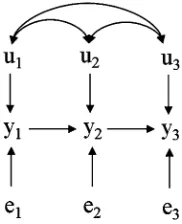
As an example, consider three traits (with phenotypesy1, y2, andy3) having the causal structure depicted in Figure 1,
where u9¼ ½u1; u2; u3 and e9¼ ½e1; e2; e3represent
ad-ditive genetic effects and residual effects, respectively. Rela-tionships among y,u, andecan be described via the SEM
8 < :
y1¼u1þe1
y2¼l21y1þu2þe2
y3¼l32y2þu3þe3;
which is similar to (1) iffixed effects are omitted, and
L¼ 2
4l021 00 00 0 l32 0
: 3 5
In addition, additive genetic and residual covariance struc-tures are given by
VarðuÞ ¼G0 ¼ 2 4 s
2
u1 su1;u2 su1;u3
su1;u2 s2u2 su2;u3
su1;u3 su2;u3 s2u3 3 5
and
VarðeÞ ¼C¼ 2 4s
2
e1 0 0
0 s2e2 0 0 0 s2e3
: 3 5
Note that as Cis diagonal, the parameters of the SEM are identifiable for any acyclic causal structure among traits. The reduced version of the SEM is
y¼ ðI2LÞ21uþ ðI2LÞ21e
¼u*þe*;
yielding:
y1¼u1þe1¼u*1þe*1
y2¼l21ðu1þe1Þ þu2þe2¼ ðl21u1þu2Þ þ ðl21e1þe2Þ ¼u*2þe*2 y3¼l32½l21ðu1þe1Þ þu2þe2 þu3þe3
¼ ðl32l21u1þl32u2þu3Þ þ ðl32l21e1þl32e2þe3Þ ¼u*3þe*3:
Note that u1, u2, and u3 represent genetic effects that
directly affecty1,y2, andy3, respectively. Further, the direct
genetic effect ony2(i.e.,u2) has an indirect effect ony3, and
genetic effects that directly influencey1(i.e.,u1) also affect y2andy3indirectly. In the SEM, the genetic effects represent
the joint effect of all genes directly contributing to variation of each phenotypic trait, but their effects are further“ trans-mitted” to other phenotypes through the causal network. While the SEM distinguishes between the direct and the indirect effects, its reduced form transforms genetic effects into effects pertaining to a model that ignores the causal association among traits, i.e., the MTM. For that reason, a genetic effect pertaining to a MTM [that is, (2) and (3)] represents the overall genetic effect exerted by the genome of the individual over each trait through all causal paths. In the example of Figure 1, the overall genetic influence on trait 2 ðu*
2Þ is obtained by reducing the model, producing
the relationship u*
2¼l21u1þu2. A fraction of u*2 is due to
a direct effect on this trait, which is represented byu2in our
SEM. Other genes may exert direct effects over trait 1 (u1),
which in turn influence trait 2 asl21u1, and therefore their
effects are included in u* 2.
As a hypothetical field example (and disregarding the actual biology involved), suppose that Figure 1 refers to three traits of sows, wherey1is litter size,y2 is the number
of live piglets at 5 days after farrowing, and y3 is total
weight of weaned pigs, all measured as traits of the sow. Because of the discrete nature of y1 and y2, this system
would be better represented by a SEM for discrete traits, but for the sake of simplicity, assume that these traits are approximately multivariate normal. For this scenario, u1
could be seen as the genetic merit of the sow regarding the size of the litter produced, which could be associated to a genetic effect on the size of the sow’s uterus or to the number of ova produced. Further, the number of live piglets at 5 days after farrowing (y2) is represented as causally
affected by litter size at the day of farrowing (y1) and by
a direct genetic effect represented by u2. This construction
implies that direct genetic effects acting over y1 would in-fluencey2indirectly, as the latter trait would also be affected
by the genetic merit for uterine size or ovulation rate. While this effect would be completely mediated by y1, some
addi-tional genetic effects could affect y2 directly (e.g., genes
affecting quality and quantity of colostrum), which are rep-resented byu2. Following the same interpretation,u3 would
represent the effect of genes on total weight of weaned pigs by the sow without mediation of both remaining traits (e.g., genes related to total volume and quality of milk produced). On the other hand, the genetic effect for weight weaned as
given by a MTM would encompass not only the effect repre-sented by u3, but also those related to prolificacy and
colos-trum. This is clear in the reduced model, where u*
3¼
l32l21u1þl32u2þu3. The same would apply tou*2, which
would contain effects of genes related to prolificacy (u*
2¼
l21u1þu2). This example illustrates that the SEM is able to
differentiate between direct and indirect genetic effects, something that cannot be accomplished via the MTM.
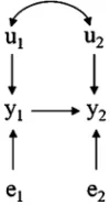
This difference between the natures of the genetic effects represented byuand byu* is reflected in the genetic cova-riances under a MTM or a SEM. In the SEM, genetic covari-ability expresses association between direct effects and can be thought of as due to genes that directly affect two traits simultaneously or to linkage disequilibrium between genes that affect two traits in a similar fashion. This is represented, for example, bysu1;u2 in the recursive model
y1¼u1þe1
y2¼l21y1þu2þe2; (4)
where
u1
u2
eN½0;G;
with
G¼
s2
u1 su1;u2
su1;u2 s2u2
as represented in Figure 2.
However, the scenario imposes a second source of genetic association between the two traits, because the genetic effect represented by u1 also affectsy2 indirectly. This
account for both sources. Therefore, even if the genes that directly affect y1 have no direct effect ony2 and were in
linkage equilibrium with the genes that actually affect y2
directly, the indirect association between u1 and y2 would
be a source of genetic covariance between the two traits under the MTM (covariance between MTM genetic effects) that is not encompassed by genetic covariances under the SEM. Nevertheless, all sources of association among traits are accounted for by the SEM via the causal connections among phenotypes. The relationship between the covarian-ces from the two models is given by
s*
u1;u2¼cov
u*
1;u*2
¼covðu1;u2þl21u1Þ ¼su1;u2þl21s2u1;
wheres*
u1;u2 is the genetic covariance under the MTM, and l21s2u1 represents the indirect genetic association among
traits, a function of the genetic variance of trait 1 and of the magnitude of the causal effect of trait 1 on trait 2.
Multiple-Trait Settings with Recursive Effects
Consider two traits involved in a network described by a recursive SEM as in Figure 2. Here, data can be analyzed by fitting a SEM with known causal structure and identifi -able model parameters or by fitting a MTM. The latter ignores the causal association between traits and is repre-sented in Figure 3.
In a selection program, one is interested in selecting candidates that result in progeny with the best expected phenotypes. Suppose we have all the information available from the SEM, including the causal structure, model param-eters, and genetic values. The vector of SEM genetic effects alone is not sufficient for predicting the expected phenotypes, but this can be done by combining this information with the causal structure and the structural coefficients. For the scenario described, assume that the magnitude of the causal relationship betweeny1 andy2is represented by a structural
coefficient with value20.5 and that both traits have the same positive economic value per unit of measurement so that subjects could be ranked using the sum of pre-dicted phenotypes for both traits as criterion. Suppose three candidates for selection, A, B, and C have SEM breeding values u9A ¼ ½2; 2;u9B¼ ½1; 3; andu9C¼ ½3; 1,
respectively. Predicted phenotypes can be obtained by inputting these values into the SEM, so they would be ranked as B, A, and C (with genetic merits ½1; 2:59, ½2; 19, and½3; 20:59, respectively). This is done by cal-culatingE½yi1;yi2jui1;ui2 ¼ ½ui1;l21ui1þui2and using the sum of predicted phenotypes as a selection criterion. Note that the direct genetic effect on trait 1 exerts a (neg-ative) effect on trait 2, while the direct genetic effect on trait 2 does not affect trait 1.
A similar analysis of the impact of each SEM breeding value on the phenotype is more awkward when the system involves more traits and more complex causal structures. However, a general method of finding the expected phenotypic
con-sequences conditionally on a vector of SEM additive genetic effects is from the relationship u*¼ ðI2LÞ21u. Therefore, the SEM make available more information than the MTM (e.g., causal relationships between traits and distinguishing between direct and indirect genetic effects), which includes the information needed to make phenotypic predictions. However, the relevant information for such predictions is given by the overall genetic effect, which is already provided by the MTM. Therefore, the MTM has the same prediction capabilities regardless of the causal model underlying the traits, which does not even need to be known. In this stan-dard framework, causal network learning would not con-tribute with additional relevant information for a breeding program.
Likewise, what genetic response is to be expected in one trait when selection is applied on the other trait? As mentioned, selection should not be based on SEM genetic effects, but on their overall phenotypic consequences. Suppose, for the same two-trait system described above, a positive correlation between direct genetic effects. If, for example, we select for subjects whose genetic effects result in more favorable y2 (i.e., larger values foru*2 under the
MTM), we would tend to select individuals who have low
u1, because that would result in decreasingy1and,
conse-quently, in an increase in y2 due to the causal association
between traits (i.e.,u1has a negative indirect effect ony2).
However, at the same time we would be selecting individ-uals with highu2, which would imply some indirect
selec-tion for highu1due to the positive SEM genetic correlation.
Therefore, selecting foru*
2would have an outcome
consist-ing of a combination of two antagonistic“influences”onu1
and, consequently, on y1. The magnitude and sign (or
di-rection) of the indirect selection for u1 would depend on
the relative magnitude of the associations represented by each path. Ultimately, the correlated response to selection would depend only on su1;u2þl21s2u1, which results from
the combination of both paths. For any causal model, these consequences can be deduced from the relationship G*
0 ¼ ðI2LÞ2
1G
0ðI2LÞ219. Again, the MTM provides the
relevant genetic covariances regardless of the causal model that generates the data, which does not even need to be known for selection purposes.
Figure 3 Diagram representing the structure of a standard bivariate model involving two traits (y1andy2) influenced by genetic effectsu*
1
andu*
2and residualse*1ande*2. Bidirected arcs connectingu*’s ande*’s
Consequences of Modifications in the Causal Model In the previous section, it was indicated that in standard frameworks of genetic improvement of multiple traits with stable causal models at the level of the phenotypes, there are no advantages from knowing the causal structure and from
fitting a SEM. Nonetheless, knowledge of the causal relation-ship among variables means being able to predict the outcome of external interventions and counterfactuals. For example, a structural equation y2¼l21y1þe2 informs the value y2
would have if the value of y1 was set toy19, but it does not
provide any information about the value ofy1after settingy2
to a different valuey29. Therefore, the advantages of using the
SEM may not be in the realm of probabilistic description of events (as they do not differ from those of the MTM), but in the prediction of effects of local interventions and modifi ca-tions in the phenotypic network (Pearl 2000, section 3.2). Therefore, the SEM can be used not only as a description of a joint distribution, but also as a description of a set of auton-omous causal mechanisms. Consequently, such models allow the prediction of the effect of local modifications in the system by making suitable changes in some equations, while keeping the remaining ones unaltered. The updated probability func-tion represents the consequences of the modification. These interventions range from changing the functional relationships between traits to simply forcing some variables to take on somefixed values, which would be mirrored as equation prun-ing and substitutprun-ing the manipulated variable by a constant (Pearl 2000, section 5.3.3). Such predictions cannot be per-formed by purely descriptive statistical models, lacking infor-mation about causal relationships among traits.
To illustrate this, assume the model with structure as in Figure 2 and suppose the same aforementioned three sub-jects A, B, and C, whose two-trait SEM breeding values given byu9A¼ ½2; 2;u9B¼ ½1; 3andu9C¼ ½3; 1, respectively, are
to be ranked. Next, consider a situation where the causal relationship between traits can be changed, for example, by an external intervention. To obtain the overall genetic effects resulting from such modifications, one can still use u*
i ¼ ðI2LÞ2
1
ui, but making suitable changes in the magni-tudes of structural coefficients inL. For example, if l21 is
changed from 20.5 to 20.9, the three ranked subjects would present MTM breeding values of ½1; 2:19,½2; 0:29, and ½3; 21:79for B, A, and C, respectively, as opposed to ½1; 2:59,½2; 19, and ½3; 20:59, respectively, for the same individuals. Note that this modification influences the expected phenotype (and consequently the expected pheno-types of the offspring), increasing the magnitude of the dif-ferences between subjects.
If the causal influence is blocked somehow, the edge between traits is removed, and the SEM becomes
y1¼u1þe1
y2¼u2þe2;
such that every entry of L would be 0, and u*
i ¼
ðI2LÞ21u
i¼ui. In this circumstance, variables that affect
trait 1 (including genetic effects represented byu1) would
not have any indirect influence on trait 2, such that genetic effects under both the SEM and the MTM are equivalent. For this scenario, the MTM genetic effects would be ½2; 29, ½1; 39, and ½3; 19 for A, B, and C, respectively, and any choice among these three would be expected to have similar overall economic consequences if the relative economic value is the same for both traits.
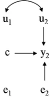
When a modification in the causal model changes the sign of the causal effect between traits, then the role of selection for trait 1 is changed. In this case, increasing the genetic effect for trait 1 would still have a desirable effect on trait 1 while having a desirable effect on trait 2 as well. If the intervention is analogous to, for example, assigning the value 0.5 to the structural coefficient, the MTM breeding values would become [3; 2.5]9, [2; 3]9, and [1; 3.5]9, for C, A, and B, which modifies the ranking for selection (B, A, and C in the original scenario). Finally, if we physically control the value of trait 1 by holding it to a constantc, then the causal influence between traits results in an average shift on trait 2. However, because the value of trait 1 is determined by an external interven-tion, the genetic effects of this trait have no influence on its phenotype (and as a consequence, there is no indirect
in-fluence on trait 2 either). Therefore, the causal structure changes to that shown in Figure 4, mirrored by a“surgery” in the SEM (Pearl 2000), which becomes
y1¼c
y2¼l21cþu2þe2:
Here, the overall mean ofy2 is shifted byl21c and animals
would be selected on the basis of differences for the direct genetic effect over trait 2 alone, because genetic merit for trait 1 does not influence the phenotypes.
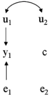
Making predictions when some variables in a causal network are physically held constant is different from making predictions based on simple conditional probabili-ties. To illustrate this, consider a different modification, in which y2 is determined by an external intervention, such
that the model becomes
y1¼u1þe1
y2¼c;
following the causal structure in Figure 5.
Here, asy2is held constant whereasy1is free to vary, the
genetic effects ony1are given byu1, so thatu1would be the
sole criterion for selection. This could be expressed as
E½y1jdoðy2¼cÞ;u2;u1 ¼E½y1ju1, wheredo() denotes that
a variable presents a given value due to external coercion. For this intervention, one might be tempted to predict y1
fromE½y1jy2;u2;u1, but the results would be different.
Ac-tually, this expression would reflect the expected value fory1
given that we observed a certain value for y2. This notion
contrasts withE½y1jdoðy2¼cÞ;u2;u1, which expresses the
expectation ofy1given thaty2 was coerced tocby an
exter-nal intervention. Predictions based onE½y1jy2;u2;u1would
be poor, since under no interventionsy2is affected byy1, so
that observingy2 updates the expectation ofy1. Conversely, y1 has no association withy2 if the value of the latter was
externally imposed, so that it should not have any bearings on the prediction. Actually, even u2 affects E½y1jy2;u2;u1,
since such expectation is expressed conditionally ony2,
mak-ing the pathy1/y2)u2active (Pearl 2000; Spirteset al.
2000). In this case, the magnitude ofu2 would mistakenly
be considered if the scenario depicted in Figure 5 holds. It should be stressed that modifications and interventions on the causal relationships between traits have an impact on the prediction of offspring’s phenotypes, which could even result in reranking of candidates for selection. As men-tioned, predicting genetic merits for scenarios where such modifications take place would not be possible using the MTM, where causal relationships are not accounted for. The modifications in breeding values get more complicated to understand as the networks become more complex, with more traits involved. However, the quantitative representa-tion of this modification can be obtained easily by transform-ing the SEM accordtransform-ing to the modification under which predictions will be made (e.g., by modifying structural
coef-ficients values or removing edges and assigning afixed value to phenotypes) and then computingðI2LÞ21ui. Therefore, the key pieces of information needed to predict breeding values under interventions in the causal model are (1) knowing how to represent the intervention or modification in theLmatrix and (2) inferring the direct genetic effect on each trait. Fitting a SEM with a suitable causal structure is necessary for that. By inferring SEM genetic effects, one could potentially predict how the genetic merits of different subjects change under a huge number of potential interven-tions or modifications in the causal relationships among traits, which is impossible when studying such systems with standard MTMs.
Following the example given inMeaning of Parameters in the SEM and the MTM, suppose that predictions are required for total weight of piglets at weaning (y3). Given the model
assumed, the genetic merit for this trait (u*
3) would be a
com-bination of direct genetic effects on the three traits in the model. However, suppose further that predictions are nec-essary for a production system that applies cross-fostering, which is an external intervention where a constant value is assigned toy2 (i.e., the same number of piglets in each litter
at 5 days after farrowing), so that this variable is no longer affected byu2 ory1 and has a constant effect ony3. Under
this intervention, the causal graph is as in Figure 6, which can be represented by the following SEM:
y1¼u1þe1
y2¼c
y3¼l32cþu3þe3:
By physically holding the value ofy2 to a constant, the
genetic effectsu1 andu2 have no indirect effects ony3; this
makes sense, as after cross-fostering, sows have an equal litter size no matter how prolific they are (which could be represented byy1) and regardless of their genetic merit for
piglet survival rate in thefirst 5 days after farrowing (which would be indicated by y2 under no intervention). Genetic
merit for total weight of weaned pigs would then depend only on direct genetic influence on this trait,e.g., via genetic merit for milk production (which could be represented by
u3). Prediction of genetic merit in such a scenario would be
possible if a study under the nonintervention scenario was made using the SEM, which would provide direct genetic effects. On the other hand, predictions based on the MTM are expected to be poor.
Another scenario illustrating the usefulness of SEM applications is that provided by studies offirst and second lactation milk yield (MY) in cows, as suggested by Gianola and Sorensen (2004). Perhaps cows with high first MY records may receive preferential nutrition and management, affecting the second lactation milk yield. This relationship consists of a positive causal influence from first to second lactation MY, with a causal structure the same as that depicted in Figure 2, wherey1 andy2 are thefirst and
sec-ond lactation MY records, respectively. The magnitude of the structural coefficient reflects the intensity of the preferential treatment. Studying the problem using the SEM instead of the MTM would allow one to predict genetic merit (or off-spring performance) of individuals in settings with different magnitudes of preferential treatment or in scenarios without preferential treatment at all, assuming there is no further source of direct causation between traits. This could be done by choosing a value of l21 that describes the scenario for
Gianola (1998), by use oft-distributed residuals in a mixed model. This may alleviate the bias in the prediction of the
“true”genetic effect, which is considered to be the genetic effect in the absence of preferential treatment. The construc-tion made here by using the SEM enables one to predict the direct genetic effects and, therefore, to obtain predictions of genetic merit that apply not only in the absence of prefer-ential treatment (the goal in Stranden and Gianola 1998), but also under different levels of preferential treatment. Furthermore, by using heterogeneous causal structures (Wuet al.2007), the various levels of preferential treatment could be accommodated in the same analysis.
Inferences for scenarios with modifications could be made also to investigate genetic association patterns. As discussed in Multiple-Trait Settings with Recursive Effects, in a simple two-trait SEM with a negative causal effect at the phenotypic level and a positive covariance between the SEM genetic effects, the sign and magnitude of a correlated response to selection applied to one trait are given by combining two antagonist paths, i.e.,su1;u2þl21s2u1. A modification in the
causal relationships among phenotypes would alter the MTM genetic covariance and, consequently, the magnitude or even the direction of the correlated response to selection. Changes in MTM genetic variances and covariances could be predicted by knowing the dispersion parameters of SEM genetic effects as well as the new value forl21. For more complex networks,
however, the consequences of modifications in the dispersion of MTM genetic effects are more difficult to follow, regardless of whether these modifications correspond to changing the magnitude of causal relationships or physically coercing a phe-notype to have a constant value. Consequences would follow from the relationshipG*
0¼ ðI2LÞ2
1
G0ðI2LÞ219. Therefore,
one can compute, for example, the magnitudes of correlated responses and heritabilities for scenarios with modified causal relationships among traits, which could not be attained by using the MTM.
Following the results of the investigation here described, we present next some examples of how the concept of intervention can make the results from previous applications of the SEM in quantitative genetics more meaningful for the context of breeding programs.
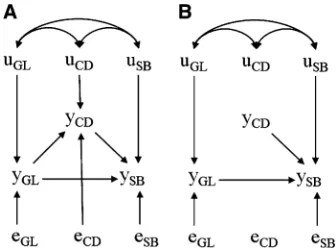
López de Maturanaet al.(2009) proposed to study three birth-related traits of primiparous Holstein cows: gestation
length (GL), calving difficulty (CD), and stillbirth (SB). CD and SB were considered as categorical traits affected by a liability variable, following a threshold model framework. A mixed-effects threshold SEM was applied, assuming a re-cursive causal structure where GL directly affected liabilities of both CD and SB directly, and the liability of CD affected the liability of SB as well. The structure considered is partially presented in Figure 7A, where systematic environmental effects and other random variables are omitted for simplicity. Due to the nonlinear relationship between GL and the re-maining traits, the magnitudes of causal associations were allowed to be heterogeneous, so that specific sets of structural coefficients were assigned according to four different inter-vals of GL values: 261–267 days, 268–273 days, 274–279 days, and 280–291 days. Although all other SEM parameters were regarded as homogeneous, assuming structural coeffi -cient heterogeneity basically results in allowing for heteroge-neity of many parameters of a reduced model.
From this causal model, it is implied that genetic effects (represented by sire genetic effects in this study) on GL affect SB via two paths: through the direct causal association between both traits (or more precisely, through the direct causal as-sociation between GL and liability for SB) and also indirectly through the liability of CD. Posterior means of inferred structural coefficients indicate that if the phenotype for GL is between 280 and 291 days, genetic effects for longer gestation would increase liability to CD, which would in turn increase liability to SB. Additionally, large genetic effects for GL in this same scenario would also increase liability for SB through the direct connection between both traits. Individual overall ge-netic effects for each trait could be obtained fromfitting a GL interval-specific MTM. However, in a context where cows undergo cesarean sections, the difficulties in calving would be externallyfixed for all females, so that gestation length would no longer affect it. Furthermore, CD would no longer be affected by its SEM genetic effects, which could possibly encompass effects of genes on pelvic area or calf frame size. By externally fixing CD, genetics would affect SB differently, because genetic effects coming from CD would be blocked, and genetic effects of GL would affect SB only through a single path instead of two. This intervention results in changing individual genetic merits for SB, but information presented by Lopez de Maturanaet al.(2009) is sufficient to predict these changes, as demonstrated next.
By fitting the SEM presented by these authors, a vector u9i¼ ½uGLi; uCDi; uSBi is assigned to each sire i.
Overall sire effect for SB could be computed as u*
SBi¼
uSBiþlSB;CDuCDiþ ðlSB;GLþlCD;GLlSB;CDÞuGLi. For GL
rang-ing from 280 to 291 days, the posterior means inferred for structural coefficients were 0.47, 0.23, and 0.60 forlCD;GL, lSB;GL, and lSB;CD, respectively. In the context under
the aforementioned intervention, the model should be mod-ified as presented in Figure 7B, such that sire effects for SB should be compared using u*
SBi¼uSBiþlSB;GLuGLi.
For example, two sires with SEM genetic effects u9A¼ ½1; 0:4; 20:04 and u9B¼ ½1; 20:4; 0:04 would have Figure 6 Hypothetical recursive causal structure as in Figure 1 after an
overall genetic effects asu*
SBA¼0:712 andu*SBB ¼0:312 on
a standard scenario, but the intervention would invert the ranking of their effects on SB, which would be then
u*
SBA ¼0:19 and u
*
SBB¼0:27, respectively. Note that
per-forming a cesarean section would result in an average shift on SB, but quantifying this shift is not necessary to compare sires’overall genetic effects for the modified scenario. Also, following the concepts presented, it is possible to study how the dispersion of random effects would change in a scenario where calvings are assisted through cesarean section. For example, the sire variance for SB would be expected to change from 2.66 to 0.56.
For the considered range of GL, lower uGLi would have
a desirable effect on SB, but individuals with low uGLi are
also more likely to present GL ,280 days. Inferences indi-cated that in this case, the causal relationship between GL and SB is expected to be modified, so that lSB;GL would
become negative. Under these circumstances, lower genetic effects for GL would have undesirable effects on SB instead of desirable effects. The information provided by this anal-ysis allows one to compare sire genetic effects, considering not only modifications due to external interventions (e.g., cesarean sections) but also those under spontaneous changes in causal relationships (controlled by the phenotype for GL) or under combinations of both types of modifications.
Similar interpretations could apply to other studies. For example, Koniget al.(2008) proposed a mixed-effects SEM with three traits measured in Holstein cows, where the in-cidence of claw disorders is affected by the test-day MY before the occurrence, but it also affects the test-day MY after the occurrence, resulting in a causal structure similar to the one displayed in Figure 1. The causal structure sug-gests that the overall genetic effect of a test-day MY can be, in part, due to genetic effects affecting incidence of claw disorders (since claw disorders affect subsequent milk
pro-duction) and also due to the genetic effect for prior milk production (since it affects the incidence of claw disorders). Fitting this model allows one to predict how eradicating claw disorders through external intervention would change genetic effects for milk production. For example, such in-tervention would be expected to change the genetic variance of test-day MY and the covariance between consecutive re-cords for this trait.
Finally, Heringstadet al.(2009) proposed a mixed-effects SEM with causal structure similar to the one presented in Figure 7A to study three traits of Norwegian Red cows: Liability to incidence of certain diseases was considered as affecting the interval from calving tofirst insemination and the liability to nonreturn rate after 56 days afterfirst insem-ination. Additionally, these two last variables presented a causal connection directed from the former to the latter. Inferences for SEM parameters would allow, for example, one to predict and compare sire effects for situations in which diseases are eradicated or in which a timed artificial insemination program would externally coerce a value for the time interval between calving and first insemination. The authors also mention that different environmental con-ditions could alter the magnitudes of causal relationships between phenotypes. By expressing the expected change as a new value for structural coefficients, one can compare overall genetic effects for many different scenarios. That would allow one to have a single set of predicted direct genetic effects and to account for genotype ·environment interaction, if such interaction can be articulated in terms of modifications in the causal relationships between traits.
Discussion
According to the theory of SEMs and MTMs, even when there are complex causal relationships among phenotypes, selecting based on breeding values and estimating corre-lated responses to selection do not require knowing the causal model. The traditional MTM would do the job by expressing the information that is necessary for this task: the overall effects of the subject’s genes over different traits and the linear associations between those effects within the same individual. However, using the SEM in a scenario with stable causal relationships among traits allows predictions of the genetic merit and of correlated response to selection conditionally on a hypothetical modification or external in-tervention in the causal model. This would be important, since inferences made under a specific scenario may not apply to different scenarios. Additionally, magnitudes of her-itabilities and covariability of breeding values for different traits could change due to intervention. Such predictions are made by representing the intervention on the causal struc-ture among phenotypes and by knowing the genetic effect directly on each trait, as well as the dispersion parameters that describe their joint distribution, which is possible by
fitting a SEM. Performing such predictions would not be possible if the analysis is done using the MTM.
As obtaining predictions for different scenarios consists essentially of predicting overall genetic effects for modified networks, one could reasonably argue that the same predic-tions could be achieved by adjusting a MTM for this new scenario or treating the same trait measured in different scenarios as distinct traits within a single MTM. In this case, accounting for causal associations between phenotypes, as well as distinguishing between direct and indirect genetic effects, would not be necessary for predictions. Nevertheless, the information carried by a mixed-effects SEM would provide two advantages: (1) Predictions for a different scenario with modifications on the phenotypic network would not require data obtained from extra scenarios, while the approach with the MTM would; and (2) even small networks can suffer a huge number of possible interventions or combinations of interventions, so that obtaining data from each possible scenario andfitting the MTM to each scenario are not feasible. On the other hand, the original SEM contains sufficient information to attain predictions that are valid for all these modified networks, and this information can be expressed parsimoniously by assigning just one set of direct genetic ef-fects for each subject (while the MTM approach would assign scenario-specific genetic effects).
By bringing up the concept of external interventions and combining it with the causal meaning of the SEM, the usefulness of this modeling approach for animal breeding applications gets clearer. Conversely, this method could be useful for other tasks, such as predicting phenotypes for individuals, instead of predicting their additive genetic effects (i.e., the expected mean phenotype of their offspring). For this purpose, combining the SEM and genomic information could allow predictions of a different effect stemming from genes: the genotypic effect (possibly accounting for nonadditive effects such as dominance and epistasis), instead of additive genetic effects as considered throughout this manuscript. From a management point of view, the information conveyed by genotypic effects would be more convenient than that from additive genetic effects for the following reason: Deciding whether each young individual should be culled, kept under standard conditions, or kept and raised under personalized management conditions depends on the effects of genes on its phenotype and not on the mean phenotype of its offspring (the latter effect would be relevant for a selection program). These two effects are not identical if nonadditive effects take place. A SEM that accounts for genotypic effects would enable predictions of phenotypes in a scenario with interventions or modifications in the causal network among phenotypes. These predictions would aid in deciding what types of system (and its external interventions) would be more suitable to each individual, as well as aiding in the aforementioned manage-ment decisions (i.e., culling, standard treatment, personalized treatment, etc.), depending on how external interventions take place.
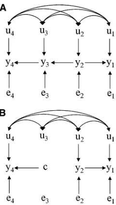
Another possible application of the concepts presented here is accounting for heterogeneous causal structures among phenotypes (Wuet al.2007), given that some of the structures
are a result of external interventions, and data are collected under different circumstances. That could be applied to the study of, for example, a system containing milk yield ðy1Þ,
feed intakeðy2Þ, incidence of estrusðy3Þ, and a fertility trait
ðy4Þ, following that feed intake affects milk yield and
inci-dence of estrus (e.g., through the active metabolism of pro-gesterone in the liver), and estrus affects fertility. Two different structures to be simultaneously accounted for in the model would be standard circumstances (Figure 8A) and a timed artificial insemination program (Figure 8B), con-sidering that in the last setting there is an external interven-tion on incidence of estrus. In this case, although the SEM would carry a single set of trait-specific direct genetic effects, both causal structures would be accounted for in the analysis and predictions for both scenarios would arise naturally, changing according to how reproduction is managed. One important issue about this system regards the uncertainty of the nature of the negative association between milk yield and reproduction: It is not established if it is as displayed in Figure 8A or if there is a direct causal effect from milk yield toward fertility. Inference of causal relationships between phenotypes is a topic currently under research by the authors, but it is outside the scope of the present article.
In this study, it was assumed that the information carried by the SEM was completely known. As the goal of this study involved understanding the usefulness of causal models that can be uncovered based on data and prior knowledge, we considered causal structures that would allow parameter identifiability from the likelihood function. Specifically, we presented recursive structures with independent residuals. In most applications that followed Gianola and Sorensen (2004), causal structures among traits were assumed known on the basis of prior knowledge on how traits are biologi-cally associated or according to temporal information. In the framework of these applications, the choice of causal struc-tures could be aided by algorithms that explore spaces of acyclic graphs (Pearl 2000; Spirteset al.2000; Valenteet al.
2010) driven by data.
It should be stressed that the aforementioned assump-tions cannot be avoided, because many distinct causal models can generate exactly the same distribution, so that the effects of interventions are not unambiguously discern-ible from data alone. Causal assumptions are necessary to establish the connection between the causal effect to be inferred and some function of data. For the SEM applica-tions, knowing the causal structures among traits is one of these assumptions, but it is not sufficient to guarantee identifiability of the causal effects. Take as an example data generated from a SEM structured as depicted in Figure 1. If inferences of causal effects are intended to be made by fi t-ting a SEM with correct causal relationship between pheno-typic traits ðy1/y2/y3Þ, but without imposing any
pair of traitsy1andy2, the requirement for the identification
of direct causal effects between them (relative to a set of traits and a causal graphGthat contains them) is given by the single-door criterion (Pearl 2000, Theorem 5.3.1). According to this criterion, and using thed-separation con-cept, the causal effecty1/y2is given by the observed
asso-ciation betweeny1andy2conditionally on a set of variablesZ
that does not contain a descendant ofy2and thatd-separates
them in a graphGl, which isGafter removing the connection
between y1 and y2. Take as an example the causal effect
betweenyGLandySBin Figure 7A. If the edge between these
traits is removed from the graph, both traits are still associ-ated through two paths: one representing the indirect effect ofyGLonySBthroughyCDand also a back-door path through
the associated genetic effects. The direct causal effects be-tween yGL andySB in a SEM structured as in Figure 7A are
identifiable because the equation forySB, aside from
present-ingyGLin the RHS, would additionally account for bothyCD
and sire effects forySB ði:e:; uSBÞ, which act as a setZ that
satisfies the conditions of the single-door criterion. In general, by postulating an acyclic causal structure and independent residuals for the SEM, this criterion would be met for the inference of every structural coefficient. However, this would not apply if residuals were not assumed as independent. For the example given, dropping this assumption would add a back-door path through eGL and eSB that could not be
blocked and would then confound inference of structural coefficients.
Considering that residuals in the SEM represent a set of the effects of variables that affect the trait in the LHS of structural equations but are not explicitly modeled, residual covariance would represent that some of these variables
affect two traits simultaneously. Accordingly, the causal meaning of postulating independent residuals is assuming that every common causal parent of two or more traits is already accounted for in the model. In the applications that followed Gianola and Sorensen (2004), the diagonal struc-ture of residual covariance matrices is generally presented as something adopted for the sake of statistical identifiability of parameters while its causal meaning is scarcely discussed. However, the causal content of this assumption is generally difficult to be absolutely guaranteed in real-world applica-tions, especially in studies of observational data, as gener-ally is the case in animal breeding.
Evidently, the assumptions involved in inferring causal effects from observational data are stronger than those required by models used simply for describing probabilities or making predictions under no interventions. However, these difficulties are actually key motivations for the study presented here. Before making decisions about using or not such models in the context of animal and plant breeding, it is imperative to investigate whether they offer any advan-tages in such contexts. It is obvious that if there were no advantages, there would be no point in using a model that accounts for causality, especially considering the challenges in meeting the requirements for identifiability of causal effects. Here, we have attempted to conduct this investiga-tion, answering the questions ofifandwhenthe information provided by such models is useful. To check how fruitful this modeling strategy can potentially be, it is important to carry out this study in the best-case scenario, where all assump-tions hold. Nevertheless, it should be stressed that we con-sidered no further or stronger assumptions in comparison to the SEM applications that followed Gianola and Sorensen (2004). As the goal of this study was to understand the relevance of these studies for breeding purposes, we ac-cepted their terms, followed their assumptions, and, using the concept of intervention, made clearer what their results would mean for breeding programs.
Because of these extra assumptions required to infer causal effects from observational data, it is harder to obtain results with the same level of certainty as, say, an estimated correlation. Conversely, standard statistical models are not exactly an alternative, because they do not provide the same information. As presented here, from data recorded under no interventions or modifications in the causal relationships between traits, predictions for genetic effects valid for scenarios under interventions cannot be provided by the MTM, regardless of how much easier it is to accept its assumptions. Additionally, abandoning the task of causal inference because assumptions cannot be absolutely guar-anteed ignores that assumptions may present a whole range of degrees of certainty. Because absolute ignorance is not the only alternative to absolute knowledge, it seems reasonable to still perform such studies with suitable care, while understanding the meaning of their assumptions and how trustworthy they are. Under more difficult situations, the SEM (and graph models in general) could still be used to Figure 8 Hypothetical recursive causal structures involving four traits (y1,
evaluate and generate hypotheses or to identify variables to be measured so that causal effects identifiability could be achieved with more confidence in future studies or even to articulate why a given causal effect is impossible to be inferred (Pearl 2000).
We focused on advantages of using the SEM in animal and plant breeding applications, where the target is to obtain predictions of genetic effects. In this regard, some extensions seem possible,e.g., developing selection index (Hazel 1943) methodologies coupled with a SEM that account for such interventions and modifications in causal networks. Here, not only the location effects may be expressed differently as direct and overall effects, but also the economic values of each trait. On the other hand, the advantages of the SEM are even clearer if the focus of the study is to explore the causal relationships among phenotypic traits, because these generally cannot be assessed via randomized experiments (Shipley 2002). By performing causal modeling involving economically important traits, it is possible to make pre-dictions of effects of external interventions, and this could be useful for farm management decisions and veterinary practices such as application of drugs and related issues.
Acknowledgments
The authors thank the two anonymous reviewers for their valuable suggestions. B.D.V. and G.J.M.R. acknowledge support from the Agriculture and Food Research Initiative Competitive grant 2011-67015-30219 from the U.S. De-partment of Agriculture National Institute of Food and Agriculture.
Literature Cited
de los Campos, G., D. Gianola, P. Boettcher, and P. Moroni, 2006a A structural equation model for describing relationships between somatic cell score and milk yield in dairy goats. J. Anim. Sci. 84: 2934–2941.
de los Campos, G., D. Gianola, and B. Heringstad, 2006b A struc-tural equation model for describing relationships between so-matic cell score and milk yield in first-lactation dairy cows. J. Dairy Sci. 89: 4445–4455.
Gianola, D., and D. Sorensen, 2004 Quantitative genetic models for describing simultaneous and recursive relationships between phenotypes. Genetics 167: 1407–1424.
Haavelmo, T., 1943 The statistical implications of a system of simultaneous equations. Econometrica 11: 12.
Hazel, L. N., 1943 The genetic basis for constructing selection indexes. Genetics 28: 476–490.
Henderson, C. R., and R. L. Quaas, 1976 Multiple trait evaluation using relative records. J. Anim. Sci. 43: 1188–1197.
Heringstad, B., X. L. Wu, and D. Gianola, 2009 Inferring relation-ships between health and fertility in Norwegian Red cows using recursive models. J. Dairy Sci. 92: 1778–1784.
Ibanez-Escriche, N., E. L. de Maturana, J. L. Noguera, and L. Varona, 2010 An application of change-point recursive models to the relationship between litter size and number of stillborns in pigs. J. Anim. Sci. 88: 3493–3503.
Jamrozik, J., and L. R. Schaeffer, 2010 Recursive relationships between milk yield and somatic cell score of Canadian Holsteins fromfinite mixture random regression models. J. Dairy Sci. 93: 5474–5486.
Jamrozik, J., J. Bohmanova, and L. R. Schaeffer, 2010 Relationships between milk yield and somatic cell score in Canadian Holsteins from simultaneous and recursive random regression models. J. Dairy Sci. 93: 1216–1233.
Konig, S., X. L. Wu, D. Gianola, B. Heringstad, and H. Simianer, 2008 Exploration of relationships between claw disorders and milk yield in Holstein cows via recursive linear and threshold models. J. Dairy Sci. 91: 395–406.
Lopez de Maturana, E., X. L. Wu, D. Gianola, K. A. Weigel, and G. J. M. Rosa, 2009 Exploring biological relationships between calving traits in primiparous cattle with a Bayesian recursive model. Ge-netics 181: 277–287.
Lopez de Maturana, E., G. l. Campos, X. L. Wu, D. Gianola, K. A. Weigel et al., 2010 Modeling relationships between calving traits: a comparison between standard and recursive mixed models. Genet. Sel. Evol. 42: 1.
Pearl, J., 2000 Causality: Models,Reasoning and Inference. Cam-bridge University Press, CamCam-bridge, UK.
Rosa, G. J. M., B. D. Valente, G. l. Campos, X. L. Wu, D. Gianola
et al., 2011 Inferring causal phenotype networks using struc-tural equation models. Genet. Sel. Evol. 43: 6.
Shipley, B., 2002Cause and Correlation in Biology. Cambridge Uni-versity Press, Cambridge, UK/London/New York.
Spirtes, P., C. Glymour, and R. Scheines, 2000 Causation, Predic-tion and Search. MIT Press, Cambridge, MA.
Stranden, I., and D. Gianola, 1998 Attenuating effects of prefer-ential treatment with Student-t mixed linear models: a simula-tion study. Genet. Sel. Evol. 30: 565–583.
Valente, B. D., G. J. M. Rosa, G. de los Campos, D. Gianola, and M. A. Silva, 2010 Searching for recursive causal structures in multivariate quantitative genetics mixed models. Genetics 185: 633–644.
Varona, L., D. Sorensen, and R. Thompson, 2007 Analysis of litter size and average litter weight in pigs using a recursive model. Genetics 177: 1791–1799.
Verma, T., and J. Pearl, 1990 Equivalence and synthesis of causal models, pp. 255–268 inProceedings of the 6th Conference on Uncertainty in Artificial Intelligence, Cambridge, MA 1990. Wright, S., 1921 Correlation and causation. J. Agric. Res. 201:
557–585.
Wu, X. L., B. Heringstad, Y. M. Chang, G. de los Campos, and D. Gianola, 2007 Inferring relationships between somatic cell score and milk yield using simultaneous and recursive models. J. Dairy Sci. 90: 3508–3521.
Wu, X. L., B. Heringstad, and D. Gianola, 2008 Exploration of lagged relationships between mastitis and milk yield in dairy cows using a Bayesian structural equation Gaussian-threshold model. Genet. Sel. Evol. 40: 333–357.
Wu, X. L., B. Heringstad, and D. Gianola, 2010 Bayesian struc-tural equation models for inferring relationships between phe-notypes: a review of methodology, identifiability, and applications. J. Anim. Breed. Genet. 127: 3–15.