GENOMIC SELECTION
Genetic Mapping and Genomic Selection Using
Recombination Breakpoint Data
Shizhong Xu1
Department of Botany and Plant Sciences, University of California, Riverside, California 92521
ABSTRACTThe correct models for quantitative trait locus mapping are the ones that simultaneously include all significant genetic effects. Such models are difficult to handle for high marker density. Improving statistical methods for high-dimensional data appears to have reached a plateau. Alternative approaches must be explored to break the bottleneck of genomic data analysis. The fact that all markers are located in a few chromosomes of the genome leads to linkage disequilibrium among markers. This suggests that dimension reduction can also be achieved through data manipulation. High-density markers are used to infer recombination breakpoints, which then facilitate construction of bins. The bins are treated as new synthetic markers. The number of bins is always a manageable number, on the order of a few thousand. Using the bin data of a recombinant inbred line population of rice, we demonstrated genetic mapping, using all bins in a simultaneous manner. To facilitate genomic selection, we developed a method to create user-defined (artificial) bins, in which breakpoints are allowed within bins. Using eight traits of rice, we showed that artificial bin data analysis often improves the predictability compared with natural bin data analysis. Of the eight traits, three showed high predictability, two had intermediate predictability, and two had low predictability. A binary trait with a known gene had predictability near perfect. Genetic mapping using bin data points to a new direction of genomic data analysis.
Q
UANTITATIVE trait loci (QTL) can be mapped to chro-mosome regions, due to the discovery of molecular markers. Early studies had few and widely spaced markers, leading to poor estimation of QTL effects. Lander and Botstein’s (1989) interval mapping has revolutionized genetic map-ping and made it possible to locate QTL in intervals be-tween observed markers. Increased marker density, along with increased sample size, can further increase the resolu-tion of QTL mapping (Wright and Kong 1997). We are now in a situation that is opposite to interval mapping: we need to delete markers with the same information content. A ge-nome is easily saturated with a few million SNPs and, as such, interval mapping is no longer required. One can simply ana-lyze markers one at a time and scan the entire genome for significant markers. This type of one-dimensional marker anal-ysis does not present a computational challenge. However, the approach is technicallyflawed if there are more than one QTL in the genome. Various modifications of the one-dimensionalscan have been proposed, such as the composite-interval map-ping (CIM) procedure (Jansen and Stam 1994; Zeng 1994). The goal of CIM is to estimate one major QTL that is detect-able and, at the same time, to correct effects from other major QTL (detectable) and the“polygenic effects”that are not de-tectable. The CIM method also faces a new challenge regard-ing how to choose the cofactors to capture the background information. The results are often unstable because different markers selected as cofactors can lead to different results.
A better approach of QTL mapping has been the multiple-interval mapping (MIM) procedure (Kao et al. 1999), in which all intervals are included as candidate regions and the actual QTL-associated intervals are searched via a step-wise regression analysis. When the marker density is too high, the number of intervals can be huge, presenting a great computational problem for the method. Therefore, the MIM method, in its original form, is no longer the best option. If one evaluates only a fixed number of positions in the ge-nome, the model dimension will not change as the marker density increases. In this case, high-density markers will further reduce the uncertainty of genotype inferences for the positions evaluated. The model dimension will increase as the number of evaluated positions increases. However, the model dimension cannot be larger than the sample size, Copyright © 2013 by the Genetics Society of America
doi: 10.1534/genetics.113.155309
Manuscript received July 12, 2013; accepted for publication August 14, 2013 Supporting information is available online athttp://www.genetics.org/lookup/suppl/ doi:10.1534/genetics.113.155309/-/DC1.
which is due to the intrinsic limitation of the maximum-likelihood method.
The Bayesian method is a better alternative to the MIM procedure (Satagopanet al.1996; Sillanpää and Arjas 1998, 1999). One major advantage of the Bayesian method is the ability to assign informative prior distribution to QTL param-eters, especially QTL effects. An informative prior will pe-nalize large estimated effects and thus shrink estimated QTL effects toward zero. The consequence of using shrinkage pri-ors is the ability to handle high-dimensional models. The MCMC-implemented Bayesian methods involve changes in model dimension, which presents another challenge because the Markov chains often take a long time to converge. In addition, the computational complexity increases when we have to manage millions of markers.
Meuwissenet al.(2001) adopted a new Bayesian method with afixed model dimension to evaluate the entire genome, using high-density SNP markers. Their purpose was not to detect QTL, but rather to predict breeding values, a new form of marker-assisted selection. Their work was not well recog-nized until recently when high-density markers became widely available in many organisms. The approach is known as “ ge-nomic selection”and has become very popular in animals and plants (Hayes et al. 2009; Heffneret al.2009) as well as in humans (Yanget al.2010) and laboratory animals (Oberet al. 2012). Xu (2003) and Wang et al.(2005) realized that this idea can be applied to line-crossing experiments for both QTL detection and genomic selection. In genomic selection, all ge-nomic positions are considered, although there is some adjust-ment for linkage disequilibrium, such as forcing positions to be atdcM apart, wheredmay be 1 or 2 (Meuwissenet al.2001). The least absolute shrinkage and selection operator (LASSO) method (Tibshirani 1996) is an alternative Bayesian method that can achieve the same goal of handling large models but has avoided MCMC samplings. In terms of computational speed, the LASSO method implemented in the GlmNet/R program (Friedmanet al.2010) is the fastest one among all other software packages. Unfortunately, even the GlmNet/R program cannot produce satisfactory results for a model con-taining a few million SNPs (Huet al.2012). It appears that statistical approaches have reached a plateau and further studies of genetic mapping via new statistical methods alone may lead nowhere.
Two research teams led by Qifa Zhang and Bin Han in China pioneered a ground-breaking work in genetic map-ping (Huang et al. 2009; Xieet al. 2010; Yu et al. 2011). They used high-density SNP markers to infer recombination breakpoints and then converted the breakpoint data into bin data. All markers within a bin have the same segregation pattern. Each bin is considered a new marker. QTL mapping is then performed using the bin data. Since the number of bins in afinite population is alwaysfinite and can be sub-stantially smaller than the original number of markers, ge-netic mapping using the bin data is much easier than that using the original markers. The model dimension can be substantially smaller, yet without loss of information. This
is an alternative dimensional reduction technique that requires no comprehensive statistical methods. The bin data analysis is potentially more useful than the original marker analysis in detection of epistatic effects (G3G) and G3E interactions. This study aims to investigate the properties of bin data and use bin data to perform QTL mapping and genomic selection.
Materials and Methods
Definition of bins
Breakpoints:We now use a recombinant inbred line (RIL)
derived from the cross of two inbred lines (diploid plants) as an example to describe the breakpoint data. Let GG3RR be the mating type of the two founding lines that initiate the cross. An RIL derived from a single-seed descent of an F1
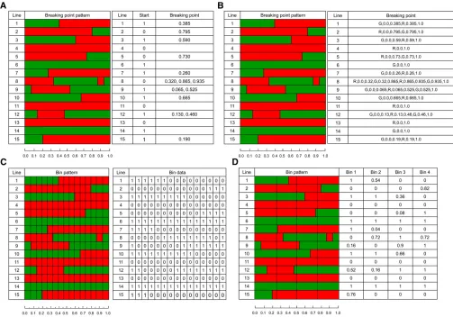
plant (GR) will be either GG or RR in genotype at this locus. If the genotypes of an RIL are color-coded green for the G genome and red for the R genome, a chromosome of the RIL will be a mosaic of the two parents, as shown in Figure 1A. Figure 1A shows the mosaic patterns of a hypothetical chro-mosome (1 M) of 15 lines. Take line 1, for example; thefirst segment (0.385 M) of the chromosome is inherited from the green parent and the second segment (0.615 M) is inherited from the red parent. The breakpoint occurs at the position where the color changes from green to red (at 0.385 M). Therefore, the genotype data of line 1 for this chromosome can be represented by a letter indicating the color of thefirst segment (G) and a single right breakpoint (0.385). If we use 1 to indicate G and 0 to indicate R, the genotype of line 1 for this chromosome is represented by two numbers, [1, 0.385]. For line 2, the genotype is represented by [0, 0.795] because the initial segment is R and the breakpoint occurs at position 0.795 M of the chromosome. Line 4 carries the entire R chromosome and thus is represented by [0] because no breakpoint exists. The genotype of line 8 can be represented by [0, 0.320, 0.865, 0.935] since it starts with R followed by three breakpoints. The breakpoint data of all 15 lines for this hypothetical chromosome are also given in Figure 1A. The initial SNP data of this chromosome may contain the geno-types of several thousand SNPs. An alternative way to pres-ent the breakpoint data is shown in Figure 1B. Each segmpres-ent is denoted by a letter (G or R) followed by the starting and ending points of the segment. For example, line 1 carries two segments, one denoted by G, 0.0, 0.385, meaning that thefirst segment comes from the G parent with starting and ending points of 0.0 and 0.385, respectively. The second segment comes from the R parent with starting and ending points of 0.385 and 1.0, respectively. Thus, the second seg-ment is denoted by R, 0.385, 1.0.
breakpoints are considered new genomic data. Development of statistical methods for breakpoint data analysis represents a new direction of quantitative genomics.
Natural bins: Breakpoint data must be converted into bin
data prior to QTL analysis (Yuet al.2011). A bin is defined as a segment that has no breakpoints within the segment across all lines in the entire RIL population. For any partic-ular bin, a line takes either the G or the R genome but not a mosaic of both. Figure 1C illustrates 15 bins for the hypo-thetical chromosome of the 15 lines. Using 1 and 0 to denote the G and R genomes, respectively, the bin genotype data for the 15 lines are illustrated in Figure 1C also. Each bin is considered a “synthetic marker”. We now have bin type data for the RIL population. The new data (bin geno-types) are then used for QTL study.
A bin defined this way is called a natural bin. Since there are no breakpoints allowed within a bin, the sizes of natural bins vary randomly from very small to very large, depending on the sample size. Natural bins are also sample specific. Introducing a new plant to the current sample may introduce new breakpoints and thus introduce new bins. Although QTL
mapping using natural bins has been proved to be very powerful (Yuet al.2011), the result may not be directly ap-plicable to marker-assisted breeding and genomic selection. Suppose that we have a natural bin with an estimated effect 3:060:25 cm in height of a crop. A plant with the green genome of this bin will be 3:060:25 cm taller than a plant that carries the red genome. If a new plant is introduced, we can predict the height of this plant based on whether this plant carries the green or the red genome for this bin. Since recom-bination events are random, by chance a breakpoint may be present in this bin for this plant, resulting in no predicted value for this plant. We may define the genotype of the new plant for this bin as the proportion of the green genome within the bin. But this will need a revision of the bin definition.
Artificial bins: In this study, we extend the bin definition to allow breakpoints to happen within bins, the so-called artificial bins. The sizes of artificial bins can be arbitrarily set according to the preference of the investigator. With the artificial bins, we can control the sizes of the bins. In ad-dition, adding new individuals will not change the pre-viously defined bins. Therefore, analysis of artificial bins can
facilitate marker-assisted breeding and genomic selection. Figure 1D shows the hypothetical chromosome with four artificial bins. The size of each bin is 0.25 M, a constant bin size. The sum of the sizes of all four bins is 1 M, equiv-alent to the length of the hypothetical chromosome.
The genotype of an artificial bin is coded differently from that of a natural bin if it contains breakpoints. It takes the proportion of the green genome of the bin. For example, thefirst bin of line 1 contains all the green genome and thus the genotype of bin 1 for line 1 is 1. The genotype of bin 2 for line 1 is 0.54 because 54% of the second bin is made of the green genome. The genotype coding of the four bins for the 15 lines is shown in Figure 1D. We now have four user-defined bins. It is important to note that genotypes of artificial bins are plant specific because they are defined as proportions. The number of artificial bins is a fixed number and does not depend on the sample size and the number of SNP markers. Clearly, adding new lines to the population will not change the number and sizes of the predefined artificial bins, making marker-assisted selec-tion more convenient.
Estimation of bin effects
Continuous genome model: Letyjbe the phenotypic value
of a quantitative trait of linejforj51;. . .; n, wherenis the number of lines. The linear model foryjis
yj5Xjb1
Z L
0
Zjlgldl1ej5Xjb1gj
L1ej; (1)
where l is a genomic location expressed as a continuous quantity, ZjðlÞ is a binary indicator variable defined as ZjðlÞ51 if j carries the green genome at position l and ZjðlÞ5 21 otherwise,gðlÞis the genetic effect at location l expressed as a function of l, Xj and b represent some covariates and their effects (systematic effects) that must be included in the model to reduce the residual error, and ejNð0;s2Þis the residual error with an unknown variance s2. The integral in Equation 1, also denoted by g
jðLÞ, is called the genomic or breeding value for individualj. This model is the continuous genome model proposed by Hu et al. (2012). The model is also called a marker-based in-finitesimal model because it implies an infinite number of loci along the genome. Their interest was to estimate the genetic effect functiongðlÞand use this function to predict the total genomic value of new lines that have not yet been phenotyped.
The model given in Equation 1 is a type of functional linear model (Cardot et al.2003; Muller and Stadtmuller 2005) in which the response variable is a scalar and the covariate is a function, which is different from the functional linear model of QTL mapping developed by Wuet al. (2004), who dealt with a functional response variable,e.g., longitudinal trait QTL mapping. Splines and polynomial curve fitting techniques commonly used in functional data analysis cannot be applied here because the QTL effect functiongðlÞis not smooth and
can be arbitrarily rough. In other words,gðl1Þandgðl2Þmay
not be correlated, even in the situation wherel1is close tol2.
In fact, there is no biological evidence that genetic effects of different loci are correlated in any form.
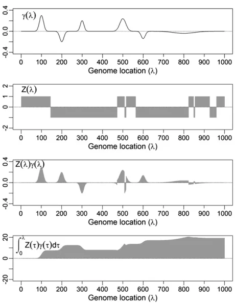
Figure 2 shows an example ofgðlÞ,ZjðlÞ,ZjðlÞgðlÞ, and the genomic value up to locationldenoted by the integral
gjl5
Z l
0
Zjtgtdt: (2)
When l5L, i.e., l reaches the end of the genome, the above integral is gjðLÞ, the genomic value for individual j. Although there is only one function for QTL effectgðlÞper population,ZjðlÞis individual specific and so is the genomic value. Function ZjðlÞ is a continuous-time discrete Markov process under certain crossover assumptions. The genomic value for this example (Figure 2, bottom) isgjðLÞ518:5.
Numerical integration: Because the function gðlÞ is un-known, the integral is not explicit and thus a form of nu-merical integration is required. Here, we used the Lebesgue– Stieltjes integral that reduces the integral into the sum of afinite number of bin effects,
yjXjb1X m
k51
Zjlk
glk
Dk1ej; (3)
Figure 2 An example showing the shapes of several variables expressed as functions of the genome location (l). The genomic value of the dem-onstrated individual isgðLÞ5RL
wheremis the number of bins,ZjðlkÞis the averageZjfor all loci within bink,gðlkÞis the average effect of all loci within this bin, andDkis the bin size. The bins can be natural bins or artificial bins defined by investigators. For equal-sized artificial bins,Dk5D for all k51;. . .; m. The symbollk represents the central location (midpoint) of the kth bin. Let us rewrite the genotype of bin k for individual j by Zjk5ZjðlkÞ and define gk5gðlkÞDk as the total genetic effect of the kth bin. We now have the following working model to estimate the genetic effect of each bin:
yj5Xjb1
Xm
k51
Zjkgk1ej: (4)
When we replace the sum of products by the product of sums, a term has been ignored, which has been explained by Hu et al.(2012) using the summation. InSupporting Information,
File S1, we provide a proof directly using the integral. Please seeFigure S1,Figure S2,Figure S3,Figure S6andFigure S7, as well asTable S5for additional information.
The model in Equation 4 has afinite dimension ofmand we have converted the infinitely high-dimensional genomic problem into a manageable working model with a finite di-mension. The statistics are now based on measured values,
which is a common theme in nonparametric and semipara-metric problems. Letqbe the length of thefixed-effect vector b. Ifm1q,n, the ordinary least-squares method can be used for parameter estimation. Ifm1q.n, a penalized regression method can be used. We choose the LASSO method devel-oped by Tibshirani (1996) and implemented in the GlmNet/R program (Friedmanet al.2010) to perform parameter estima-tion. Of course, any methods that efficiently handlen individ-uals andmbins can be used for parameter estimation. Significance tests of bin effects
Let ^gk be the estimated effect for binkand varðg^kÞ be the variance of g^k. The most convenient test is the Wald test defined as
Wk5 ^gk varð^gkÞ;
(5)
which is similar to the likelihood-ratio test (LRT) statistic, and the two are often used interchangeably ifg^kis normally distributed. The LRT can be converted into the log of odds (LOD) score, using
LODk5 Wk 2lnð10Þ
Wk
4:61: (6)
Two issues need to be addressed for the test. One is how to calculate varð^gkÞfor the shrinkage estimate and the other is how to correct multiple tests for genome-wide study. By shrinkage estimates of bin effects, we refer to the LASSO estimates of all bin effects in a simultaneous manner. If m1q,n and a multiple-regression method is applied, varðg^kÞ has a standard formula. When m1q.n and the LASSO method is applied, there is no explicit formula to calcu-late varðg^kÞ. Letg^kbe the LASSO estimate and varðg^kÞbe the variance of the estimate. They are interpreted as the Bayesian posterior mean and posterior variance, respectively. We pro-pose the following approximate method to calculate varð^gkÞ,
var^gk
5 s^2ks^2 ^
s21s^2
kZTkZk
; (7)
where
^
s251
n
y2X^b2Z^gTy2Xb^2Z^g (8)
is the estimated residual variance and
^
s2
k5 ^
g2
kZTkZk1
ffiffiffiffiffiffiffiffiffiffiffiffiffiffiffiffiffiffiffiffiffiffiffiffiffiffiffiffiffiffiffiffiffiffiffiffiffiffiffiffiffiffiffiffiffiffiffiffiffiffiffi
^
g2kZT kZk
2
14s^2g^2
kZkTZk
q
2ZkTZk (9)
is a“prior”variance ofgk. Derivations of the above formulas are given inFile S2. The principle underlying the derivation is the Bayesian posterior variance. The critical value of the Wald test used to declare statistical significance is drawn from the permutation test (Churchill and Doerge 1994). How-ever, as shown in Results, multiple-tests correction seems to be unnecessary under the shrinkage estimation, which is in contrast to genome-wide QTL detection under the single-marker model analysis.
Genomic selection
The bin data can be used to predict breeding values. The method of parameter estimation remains the same as described before. Here, we skip the bin effect detection step and use all bins, regardless of the sizes of the bin effects, to predict the genomic values of future individuals that have yet to be phenotyped. In genomic selection, artificial bins must be used because newly added individuals will in-troduce new bins whose effects are not yet evaluated in the testing sample. Note that artificial bins are used only for genomic selection and not for QTL detection because there are no breakpoints within natural bins (across individuals). As is well known in regression analysis, it is harder to de-tect the regression coefficient for a predictor with a small variance across observations than that for a predictor with a large variance. On the other hand, combining small bins together may substantially reduce the model dimension, which in turn may increase the model stability and thus improve predictability relative to the natural bin analysis. The variance of an artificial bin is inversely related to the bin
size. If an artificial bin is not substantially large, the variance reduction may be trivial and thus lead to negligible loss in predictability. For an RIL population initiated from two inbred lines withZjðlÞ51 andZjðlÞ5 21 representing the two alternative genotypes, the variance of the artificial bin genotype indicator for bin kis
varðZkÞ5var½ZðDkÞ
5 1
2D2k n
j21 2e22Dk
12ln2Dk1121 h
6ðlnð2ÞÞ22p2
io
;
(10)
where
j2x5X N
i51
xi
i2 (11)
is the dilogarithm function. Derivation of Equation 10 along with the variances in various other populations is given in
File S3. The limits of the variance are lim Dk/0
var½ZðDkÞ51
and lim Dk/N
var½ZðDkÞ50. The situation ofDk/0 is
equiva-lent to a single fully informative marker with the maximum variance of 1. When the bin size is 0.01 M, i.e.,Dk50:01, the corresponding variance is var½Zð0:01Þ50:98685, which presents a negligible reduction. A genome with 30 M in length would give 3000 equal-sized bins with a length of 1 cM. A model with 3000 effects can be easily handled by most penalized regression methods.
In real data analysis, the bin size can be determined using theK-fold cross-validation. The ideal bin size should be the one that gives the smallest mean squared error (MSE),
MSE51 n
Xn
j51
yj2Xjb^2X m
k51
Zjkg^k
2
: (12)
This cross-validation-generated MSE differs froms^2, the
es-timated residual error variance, in that individuals predicted never contribute to the estimation of parameters used to
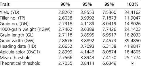
Table 1 Empirical threshold values of the likelihood-ratio test statistics of the LASSO method
Trait 90% 95% 99% 100%
Yield (YD) 2.8262 3.8553 7.5360 34.4162
Tiller no. (TP) 2.6038 3.9392 7.1873 11.9047
Grain no. (GN) 2.7318 4.1189 8.0419 14.8026
1000-grain weight (KGW) 2.7462 3.6388 7.7426 24.1423
Grain length (GL) 2.7118 3.8595 6.9517 16.2033
Grain width (GW) 2.8676 3.8892 7.4573 39.4850
Heading date (HD) 2.6652 3.7093 6.3158 41.9847
Apicule color (OsC1) 2.8999 4.1446 8.0874 18.4805
Mean threshold 2.7566 3.8943 7.4150 25.1774
Theoretical threshold 2.7055 3.8414 6.6349 N
predict the phenotypes of these individuals. The estimated residual error variance is often close to zero because the model overfits the data. To get a more useful sense of model uncertainty, we use cross-validation to draw MSEs. A smaller MSE means a higher predictability. Two alternative measure-ments of model predictability are cross-validation-generated R2obtained through
R21512MSE MSP andR
2 25
cov2y;^y
varðyÞvarð^yÞ; (13)
where MSP5varðyÞ is the observed phenotypic variance and varð^yÞis the variance of the predicted phenotypic val-ues. The secondR2is simply the squared Pearson correlation
coefficient between the observed and predicted trait values. A higherR2means a better predictability.
We expected that the natural bin analysis would perform better than the artificial bin analysis in terms of minimizing MSE or maximizingR2. We hope tofind suitable equal-sized
artificial bins so that the MSE is close to that of the natural bin analysis. This will justify the artificial bin analysis as an efficient substitute for the natural bin analysis so that the result of artificial bin analysis can be applied conveniently to genomic selection.
Experimental material
We used 210 recombinant inbred lines of rice (Oryza sativa) with eight traits (Yu et al.2011) to illustrate the method. The two founders were Zhenshen97 and Minghui63, and both areindica subspecies. A total of 270,820 high-quality SNPs were identified in the experiment, yielding a genome-wide SNP density of1 SNP/1.37 kb. These SNPs were used to infer the breakpoints of each RIL, resulting in a total of 1619 natural bins (no breakpoints within bins). The frequency distribution of the bin size is shown in Figure 3, top, which appears to be exponential. The distribution of the log bin size is shown in Figure 3, bottom. The minimum and maximum sizes of the natural bins are 0.006 Mb and 7.95 Mb, respec-tively, with a mean of 0.23 Mb. In the original analysis of Yu et al.(2011), each bin was treated as a marker. Genetic link-age analysis of these bins showed that the total length of the rice genome is 1625.5 cM in length, equivalent to 1.0 cM per bin. The physical length of the rice genome is430 Mb (Chen et al.2002). The starting and ending points of each natural bin were also provided by the original authors (Yuet al.2011).
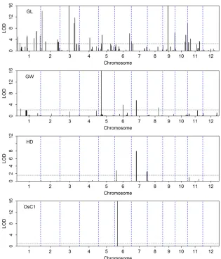
Eight traits were analyzed, including yield per plant (YD), tiller number per plant (TP), grain number per panicle (GN), 1000-grain weight (KGW), grain length (GL), grain
width (GW), heading date (HD), and apicule color (OsC1). The first seven traits are quantitative and the last one is binary. The binary color trait is controlled by a single gene on chromosome 6 (bin 868), named OsC1, and has been cloned by the authors. Thefirst four traits (YD, TP, GN, and KGW) were replicated four times (two locations in 2 years), and GL and GW were replicated twice (2 different years). HD was replicated three times (3 different years). OsC1 was not replicated. For traits with replications, the phenotypic value took the average of the replicates, after adjusting for the systematic differences of the replicates as fixed effects. Therefore, we detected only the main effects and ignored the potential G3E interaction effects.
Results
Detection of associated bins
The sample size isn5210 and the number of natural bins is m51619. The model for the natural bin analysis is given in Equation 4, where b is the intercept because the environ-mental effects were already removed prior to the analysis. We used the LASSO method implemented in GlmNet/R
(Friedman et al.2010) for data analysis. After the analysis of the original data, we performed permutation tests. We generated 1000 permuted samples where the phenotypic values of the 210 lines were randomly shuffled so that the association of the phenotype with any bin is purely caused by chance. For each permuted sample, we recorded the largest Wald test score among the 1619 bins. The largest Wald test scores from the 1000 permuted samples formed a null distribution. We choose the 95th percentile of this null distribution as the critical value. These threshold values are shown in Table 1 along with the thresholds of 90th, 95th, 99th, and 100th percentiles. To our surprise, the average 95% threshold value of the eight traits is 3.8943, which is not much different from 3.8414, the theoretical 95% thresh-old of a Chi-square distribution with one degree of freedom. This may be coincidental, but all eight traits show similar threshold values (with very little variation). This implies that there is no need for multiple-test correction under the shrinkage method. Of course, more investigation will be needed to draw a general conclusion. A nominal P50:05 can be used to declare statistical significance for all bins with the LASSO method. If investigators prefer a more conserva-tive test, the 99% critical value can be used. The average
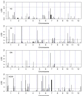
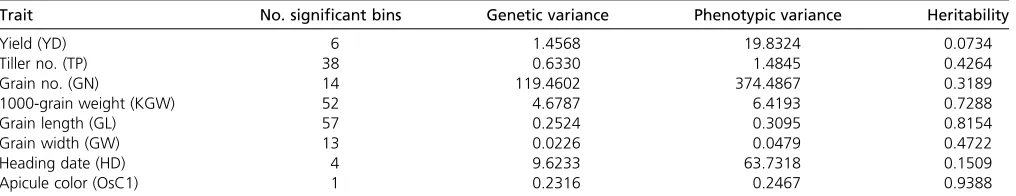
99% threshold value for the eight traits is 7.415, slightly over 6.6349, the theoretical value of 99% for the Chi-square distribution with one degree of freedom (see Table 1). Using trait-specific 95% threshold values, we present the LOD score test statistics for thefirst four traits (YD, TP, GN, and KGW) in Figure 4 and for the last four traits (GL, GW, HD, and OsC1) in Figure 5. The number of bins detected and the proportion of phenotypic variance explained by the associated bins are listed in Table 2 for each of the eight traits. YD and HD are low-heritability traits and the numbers of associated bins are also small for the two traits (6 and 4). All 6 bins associated with yield have LOD score,2 and collectively explain only 7% of the trait variation. If more stringent (conservative) criteria were used, none of them would be significant. TP, GN, and GW have intermediate heritability with intermediate numbers of associated bins (38, 14, and 13). KGW and GL are highly heritable with a large number of associated bins for each trait (52 and 57). The apicule color trait is known to be controlled by a cloned gene (OsC1), which is indeed detected by the LASSO method with a LOD score near 50,000. The reason that the proportion of phenotypic variance explained by this single bin is not 100% is due to the fact that we treated the binary trait as continuous and ignored the binary nature of the trait. Including this single-gene-controlled binary trait in the analysis proved that the LASSO method is efficient in QTL detection for both polygenic and monogenic traits.
The estimated effects, the standard errors, the LOD scores, and theP-values for all 1619 bins are provided inFile S4. Yu et al.(2011) reported QTL mapping results for thefirst four traits (YD, TP, GN, and KGW) and the binary color trait (OsC1), using the CIM procedure (Jansen and Stam 1994; Zeng 1994). We compared our LOD scores with theirs and discovered some similarities and differences between the two analyses. In principle, the two analyses are not comparable because they aimed to detect environment-specific QTL and we targeted main-effect QTL. Yuet al.(2011) did notfind any QTL that appeared in two or more environments for YD and TP; i.e., all QTL are environment specific for the two traits. However, they detected three QTL for GN and six QTL for KGW that occurred at least in two environments and some occurred in all four environments. These so-called “ main-effect”QTL detected by Yuet al.(2011) are all detected in our analysis. For example, we detected a large main-effect QTL for KGW on chromosome 5 (bin 729) with a LOD score.150
and explaining 15.4% of the phenotypic variance. This large QTL was detected in all four environments by Yuet al.(2011).
Comparison with composite-interval mapping
As requested by a reviewer and the editor, we used the CIM method implemented in the R/qtl program (Broman et al. 2003) to reanalyze the eight traits. The cim() function of the program was used with default settings for the argument values. We compared the LASSO method with the CIM method only for the natural bin data (not the artificial bins). In addition, we also compared the results with the interval mapping (IM) procedure for the natural bins. First, we ex-amined the permutation-generated percentiles for the LRT test statistics for the IM procedure (seeTable S1). There is very little variation across different traits for each percentile. The average percentile values across traits are 13.82, 15.45, 19.11, and 25.67, respectively, for 90%, 95%, 99%, and 100%. These values are way over the nominal thresholds for the Chi-square distribution with one degree of freedom. To control the genome-wide type I error rate at 0.05, the LRT must be.15.45, much higher than the theoretical nom-inal level of 3.84. This critical value converts to a LOD score of 15:45=4:6153:35. For the CIM procedure, the permutation-generated threshold values are, on average across traits, 17.46, 19.52, 23.74, and 29.78, respectively, for 90%, 95%, 99%, and 100%. To our surprise, they are even higher than those for the IM method. We can declare significance for a bin only if its LOD score is .19:52=4:6154:23. At this point, we feel more confident that the low critical value drawn from the LASSO method is not coincidental. The trait-specific thresholds in the additional analyses are listed inTable S1for the IM procedure and inTable S2for the CIM procedure.
The LOD score profiles for the eight traits obtained from the three methods (LASSO, CIM, and IM) are plotted in
Figure S4(thefirst four traits) andFigure S5(the last four traits). Overall, many regions of the genome consistently show significant peaks for the three methods. The LASSO LOD score profiles often show very sharp peaks and detected substantially more bins than the other two methods. The LOD score profiles of the IM procedure always show wider peaks than the LOD score profiles of the CIM procedure, further proving the advantages of CIM over the IM proce-dure. But neither method is competitive with the LASSO
Table 2 Numbers of natural bins associated with eight traits in rice
Trait No. significant bins Genetic variance Phenotypic variance Heritability
Yield (YD) 6 1.4568 19.8324 0.0734
Tiller no. (TP) 38 0.6330 1.4845 0.4264
Grain no. (GN) 14 119.4602 374.4867 0.3189
1000-grain weight (KGW) 52 4.6787 6.4193 0.7288
Grain length (GL) 57 0.2524 0.3095 0.8154
Grain width (GW) 13 0.0226 0.0479 0.4722
Heading date (HD) 4 9.6233 63.7318 0.1509
Apicule color (OsC1) 1 0.2316 0.2467 0.9388
method. We now use YD and KGW as examples to illustrate the differences among the three methods. For trait YD, the LASSO method detected at least six significant bins while CIM detected only one wide region on chromosome 7. The IM procedure detected one more bin on chromosome 1, in addi-tion to the same region on chromosome 7. Both regions (chro-mosomes 1 and 7) were detected by the LASSO method. For trait KGW, the bin with the largest LOD score on chromosome 5 was detected by all three methods. The LASSO method pointed to a single bin but the IM and CIM procedures showed a wide region of significance and their LOD scores are not as high as that of the LASSO method. The actual LOD score test statistics for the IM procedure along with the permutation-generatedP-values for all 1619 bins are provided inFile S5. The corresponding LOD scores andP-values for the CIM pro-cedure are listed inFile S6. Interested readers may download
File S5andFile S6for further comparisons.
Genomic selection
Wefirst evaluated genomic selection for natural bins, using the 10-fold cross-validation to draw MSEs andR2’s. The results are
listed in Table 3 (top section). The two types of R2are very
close to each other. Therefore, we focus on the PearsonR2only
in subsequent discussion. TheR2values are all higher than the
heritability estimates presented early in the association study except for trait GL, where the heritability is 0.815 but the cross-validation-generatedR2¼0.79. Another important
dis-covery is that the heritability estimate for GW is 0.47 but the cross-validation-generatedR2¼0.73, a dramatic increase. This
trait would benefit the most by performing genomic selection. TheR2value for OsC1 is 0.98, a nearly perfect prediction.
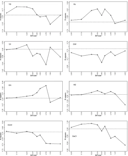
In reality, artificial bins have to be used to perform genomic selection because the bin sizes are predefined by breeders via cross-validation studies. We evaluated the following sizes of bins to select the“optimal”bin size for each trait: 0.05, 0.1, 0.2, 0.3, 0.4, 0.5, 0.75, 1.0, and 2.0, where the bin size is measured in megabases for convenience. The numbers of bins corresponding to these sizes are 7451, 3729, 1869, 1247, 938,
750, 501, 379, and 191. Figure 6 gives the plot of the squared Pearson correlation coefficient against bin size for each trait. The predictabilities of all bin sizes are less than that of the natural bin analysis for trait GW. The optimal bin size that gives the closestR2to the natural bin analysis is 2.0 Mb with
R2¼0.7291 while theR2of the natural bin analysis is 0.7344.
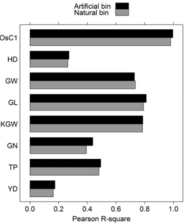
This reduction of predictability is almost negligible. According to the 0.23-Mb/1-cM ratio reported by Yu et al.(2011), 2.0 Mb is equivalent to 2:0=0:2358:6956 cM, corresponding to Dk50:086956 and var½ZðDkÞ50:8971. This reduction in variance (from 1.0 to 0.8971) may contribute to the reduction in predictability (from 0.7344 to 0.7291). The KGW trait anal-ysis also showed that artificial bin analysis does not improve the predictability compared with natural bin analysis. The op-timal bin size is 0.05 Mb with predictability 0.7871, almost the same as predictability 0.7848 in the natural bin analysis. Each of the remaining traits showed improvement in predictability at some bin sizes evaluated relative to the natural bin analysis. We did not expect to see such improvement when we started this project. The improvement may come from the merge of some very small natural bins into a larger artificial bin. The MSEs andR2’s of artificial bin analysis under the optimal bin
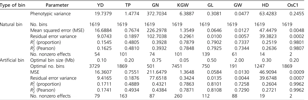
sizes are listed in Table 3 (bottom section), in which the pre-dictability of artificial bin analysis is numerically compared with that of the natural bin analysis for each trait. The corre-sponding graphical comparison is illustrated in Figure 7. The comparisons between artificial bin analysis and natural bin analysis for the estimated heritability are given inFigure S8. The estimated effects, the standard errors, the LOD scores, and theP-values for all the artificial bins are provided inFile S7, where the number of bins varies across the traits.
Discussion
Existing methods are hampered by the scale of computation introduced by dense markers. These dense markers primar-ily provide breakpoints, and data-reduction methods that take advantage of this are sorely needed. This is actually
Table 3 Comparison of natural bin and artificial bin analyses for eight traits in rice
Type of bin Parameter YD TP GN KGW GL GW HD OsC1
Phenotypic variance 19.7379 1.4774 372.7034 6.3887 0.3081 0.0477 63.4283 0.2455
Natural bin No. bins 1619 1619 1619 1619 1619 1619 1619 1619
Mean squared error (MSE) 16.6884 0.7674 226.2978 1.3549 0.0646 0.0127 47.4479 0.0048
Residual error variance 9.0743 0.1897 102.7038 0.2961 0.0100 0.0057 39.3823 0.0002
R2
1(proportion) 0.1545 0.4805 0.3928 0.7879 0.7902 0.7337 0.2519 0.9801
R2
2(Pearson) 0.1625 0.4810 0.3932 0.7848 0.7925 0.7344 0.2636 0.9807
No. nonzero effects 54 101 74 101 139 61 14 2
Artificial bin Optimal bin size (Mb) 0.10 0.20 0.75 0.05 0.50 2.00 0.30 0.20
Optimal no. bins 3729 1869 501 7451 750 191 1247 1869
MSE 16.3607 0.7551 211.6479 1.3648 0.0584 0.0130 46.9094 0.0009
Residual error variance 9.4165 0.1876 77.6518 0.3424 0.0135 0.0044 39.6748 0.0007
R2
1(proportion) 0.1711 0.4889 0.4321 0.7863 0.8101 0.7258 0.2604 0.9962
R2
2(Pearson) 0.1741 0.4934 0.4384 0.7871 0.8108 0.7290 0.2721 0.9962
No. nonzero effects 79 163 87 260 112 88 19 2
YD, yield per plant; TP, tiller number per plant; GN, number of grains per panicle; KGW, 1000-grain weight; GL, grain length; GW, grain width; HD, heading date; OsC1, apicule color (a binary trait controlled by a single gene that has been cloned);R2
1(proportion)¼1–MSE/phenotypic variance (proportion of phenotypic valiance explained by markers);R2
a statistical problem, although it uses the biological process of recombination. Using the biological process, we may divide the genome into a finite number of intervals and select one representative marker from each interval (Ober et al.2012). This type of marker selection is subjective and may not guarantee that all information is extracted from the markers. The bin data analysis is the optimal approach of data reduction without loss of information. For example,
the 270,000 SNPs of the rice population investigated in this study are fully represented by the 1619 bins. Any penalized regression methods currently available should work well for a model with this size. We choose the LASSO method (Tibshirani 1996) because the GlmNet/R program (Friedmanet al.2010) is extremely fast and we were able to use permutation tests to draw the critical values for the test statistics.
It has been a common practice to correct multiple tests in QTL mapping and genome-wide associate studies (Moskvina and Schmidt 2008; Johnsonet al.2010). The simplest way of correcting multiple tests is the Bonferroni correction, al-though it is known to be too conservative. This study shows that if QTL effects are estimated and tested simultaneously using a shrinkage method, no Bonferroni correction should be used. The nominal P-value of 0.05 should be used to declare significance for all effects of the entire genome, re-gardless of how many effects are tested. This conclusion was obtained empirically from the results of permutation tests (see Table 1), not from theoretical derivation. An intuitive explanation is that when all effects are included in a single model, the estimated effects and the test statistics tend to be small due to shrinkage, which has implicitly taken into ac-count multiple tests.
If a slightly more conservative test is preferred, one can use an alternative Bonferroni correction that uses the effective number of tests to correct the multiple tests (Moskvina and Schmidt 2008). The effective number of tests is estimated based on the linkage relationship of the markers and can be substantially smaller than the actual number of tests. How-ever, the LASSO or Bayesian shrinkage method tends to generate many zero or close to zero estimated effects. This suggests a different way of drawing the effective number of tests (Mackay 1992; Tipping 2001), where each effect is assigned a degree of confidence that is determined by the complement of the ratio of the posterior variance to the prior variance. The sum of the confidences of all effects gives the effective number of tests (seeFile S2for details). The degree of confidence is quite similar to the QTL intensity of the reversible-jump MCMC-implemented Bayesian method (Sillanpää and Arjas 1998, 1999). The effective numbers of tests for all
eight traits are listed in Table S3. For example, the OsC1 trait is known to be controlled by a single gene and the effective number of tests is 1.21, which is substantially less than 1619. The Bonferroni-correctedP-value at the 0.05 level should be 0:05=1:2150:04125;i.e., a bin can be declared as significant if the calculated P-value is,0.04125. The num-bers of significant bins using this (effective number) Bonferroni-corrected test are listed inTable S4. There is no significant bin for the yield trait. This test is more conservative than the one without the multiple-test correction.
We investigated the breakpoint and bin data analysis, using an RIL population derived from two parents as an example. Extension to multiple-parents-initiated RIL populations is straightforward. These types of data are already available in the collaborative cross (CC) mouse population (Collaborative Cross Consortium 2012) and the diversity outcross (DO) panel derived from the CC mice (Svensonet al.2012). Application of the method to the multiparent advanced-generation intercross (MAGIC) population (Kover et al. 2009) is also simple. The breakpoint pattern, the natural bins, and the artificial bins of a small hypothetical sample of a MAGIC population are illus-trated in Figure S9. There is an urgent need to develop cor-responding statistical methods for QTL mapping using bin data in this type of population.
For random populations where breakpoints are not available, we may still define bins using linkage disequilib-rium (LD) as the criterion. For example, we may calculate all pairwise linkage disequilibrium parameters for all markers of the genome. We then define a bin so that all markers within the bin have an average LD greater than a fixed number (LD criterion). A low LD criterion means a high number of bins and vice versa. The bin genotype indicator variable is the mean of the genotype indicator variables for all markers within the bin. For example, let
Zjs5
8 < :
11 0
21 for for for
A1A1
A1A2
A2A2
(14)
be the genotype indicator variable for individualjat SNPs within a bin of interest. Let nb be the total number of
markers within this bin; the bin genotype indicator variable for this individual is then defined by
Zj51 nb
Xnb
s51
Zjs: (15)
If markers within the bin are in low LD, positive and negative marker genotype indicator variables tend to cancel out each other, leading to a close to zeroZj. However, if the markers are in high LD, the majority of the markers will take the same values (coded values in the same direction), andZj will be informative to represent the bin. This explains why high LD is required to construct bins and perform the bin model association studies. In the situation where the LD level is extremely low, the number of bins can still be very
large. A weighted average bin indicator may be used, as demonstrated by Huet al.(2012).
For thefirst time, we investigated the properties of bins in terms of theoretical variance of the mean genotype indicator variable and showed how this variance affects the result of bin data analysis. We also proposed the concept of“artificial bin”to control the bin sizes and to facilitate genomic selec-tion. The artificial bin data analysis showed that it is often more efficient than the natural bin data analysis. The gain cannot be through dividing a large natural bin into several smaller artificial bins; rather, it is more likely achieved by combining several small natural bins into a larger artificial bin. This work will stimulate more theoretical and experimen-tal studies of bin data.
Acknowledgments
The author is grateful to two anonymous reviewers for their detailed comments on the manuscript. The author also appreciates Qifa Zhang for sharing some additional data beyond the data posted on the journal website for the RIL population of rice. This project was supported by the U.S. Department of Agriculture National Institute of Food and Agriculture grant 2007-02784.
Literature Cited
Broman, K. W., H. Wu, S. Sen, and G. A. Churchill, 2003 R/qtl: QTL mapping in experimental crosses. Bioinformatics 19: 889– 890.
Cardot, H., F. Ferraty, and P. Sarda, 2003 Spline estimators for the functional linear model. Stat. Sin. 13: 571–591.
Chen, M., G. Presting, W. B. Barbazuk, J. L. Goicoechea, B. Blackmon
et al., 2002 An integrated physical and genetic map of the rice genome. Plant Cell 14: 537–545.
Churchill, G. A., and R. W. Doerge, 1994 Empirical threshold values for quantitative trait mapping. Genetics 138: 963–971. Collaborative Cross Consortium, 2012 The genome architecture
of the Collaborative Cross mouse genetic reference population. Genetics 190: 389–401.
Friedman, J., T. Hastie, and R. Tibshirani, 2010 Regularization paths for generalized linear models via coordinate descent. J. Stat. Softw. 33: 1–22.
Hayes, B. J., P. J. Bowman, A. J. Chamberlain, and M. E. Goddard, 2009 Invited review: genomic selection in dairy cattle: prog-ress and challenges. J. Dairy Sci. 92: 433–443.
Heffner, E. L., M. E. Sorrells, and J.-L. Jannink, 2009 Genomic selection for crop improvement. Crop Sci. 49: 1–12.
Hu, Z., Z. Wang, and S. Xu, 2012 An infinitesimal model for quantitative trait genomic value prediction. PLoS ONE 7: e41336.
Huang, X., Q. Feng, Q. Qian, Q. Zhao, L. Wanget al., 2009 High-throughput genotyping by whole-genome resequencing. Ge-nome Res. 19: 1068–1076.
Jansen, R. C., and P. Stam, 1994 High resolution of quantitative traits into multiple loci via interval mapping. Genetics 136: 1447–1455.
Johnson, R. C., G. W. Nelson, J. L. Troyer, J. A. Lautenberger, B. D. Kessing et al., 2010 Accounting for multiple comparisons in a genome-wide association study (GWAS). BMC Genomics 11: 724.
Kao, C.-H., Z.-B. Zeng, and R. D. Teasdale, 1999 Multiple in-terval mapping for quantitative trait loci. Genetics 152: 1203–1216.
Kover, P. X., W. Valdar, J. Trakalo, N. Scarcelli, I. M. Ehrenreich
et al., 2009 A multiparent advanced generation inter-cross to
fine-map quantitative traits in Arabidopsis thaliana. PLoS Genet. 5: e1000551.
Lander, E. S., and D. Botstein, 1989 Mapping Mendelian factors underlying quantitative traits using RFLP linkage maps. Genet-ics 121: 185–199.
MacKay, D. J. C., 1992 Bayesian interpolation. Neural Comput. 4: 415–447.
Meuwissen, T. H. E., B. J. Hayes, and M. E. Goddard, 2001 Prediction of total genetic value using genome-wide dense marker maps. Genetics 157: 1819–1829.
Moskvina, V., and K. M. Schmidt, 2008 On multiple-testing cor-rection in genome-wide association studies. Genet. Epidemiol. 32: 567–573.
Muller, H.-G., and U. Stadtmuller, 2005 Generalized functional linear models. Ann. Stat. 33: 774–805.
Ober, U., J. F. Ayroles, E. A. Stone, S. Richards, D. Zhu et al., 2012 Using whole-genome sequence data to predict quantita-tive trait phenotypes inDrosophila melanogaster. PLoS Genet. 8: e1002685.
Satagopan, J. M., B. S. Yandell, M. A. Newton, and T. C. Osborn, 1996 A Bayesian approach to detect quantitative trait loci using Markov chain Monte Carlo. Genetics 144: 805– 816.
Sillanpää, M. J., and E. Arjas, 1998 Bayesian mapping of multiple quantitative trait loci from incomplete inbred line cross data. Genetics 148: 1373–1388.
Sillanpää, M. J., and E. Arjas, 1999 Bayesian mapping of multiple quantitative trait loci from incomplete outbred offspring data. Genetics 151: 1605–1619.
Svenson, K. L., D. M. Gatti, W. Valdar, C. E. Welsh, R. Cheng
et al., 2012 High-resolution genetic mapping using the
mouse diversity outbred population. Genetics 190: 437– 447.
Tibshirani, R., 1996 Regression shrinkage and selection via the Lasso. J. R. Stat. Soc. B 58: 267–288.
Tipping, M. E., 2001 Sparse Bayesian learning and the relevance vector machine. J. Mach. Learn. Res. 1: 211–244.
Wang, H., Y. Zhang, X. Li, G. L. Masinde, S. Mohan et al., 2005 Bayesian shrinkage estimation of quantitative trait loci parameters. Genetics 170: 465–480.
Wright, F. A., and A. Kong, 1997 Linkage mapping in experimental crosses: the robustness of single-gene models. Genetics 146: 417–425. Wu, R. L., C. X. Ma, M. Lin, and G. Casella, 2004 A general frame-work for analyzing the genetic architecture of developmental characteristics. Genetics 166: 1541–1551.
Xie, W., Q. Feng, H. Yu, X. Huang, Q. Zhaoet al., 2010 Parent-independent genotyping for constructing an ultrahigh-density linkage map based on population sequencing. Proc. Natl. Acad. Sci. USA 107: 10578–10583.
Xu, S., 2003 Estimating polygenic effects using markers of the entire genome. Genetics 163: 789–801.
Yang, J., B. Benyamin, B. P. McEvoy, S. Gordon, A. K. Henderset al., 2010 Common SNPs explain a large proportion of the herita-bility for human height. Nat. Genet. 42: 565–569.
Yu, H., W. Xie, J. Wang, Y. Xing, C. Xuet al., 2011 Gains in QTL detection using an ultra-high density SNP map based on popu-lation sequencing relative to traditional RFLP/SSR markers. PLoS ONE 6: e17595.
Zeng, Z.-B., 1994 Precision mapping of quantitative trait loci. Genetics 136: 1457–1468.