Improving the Accuracy and Efficiency of Identity-by-Descent Detection in Population Data

(1)

INVESTIGATION

Improving the Accuracy and Ef

ﬁ

ciency

of Identity-by-Descent Detection in Population Data

Brian L. Browning*,1_{and Sharon R. Browning}†

*Department of Medicine, Division of Medical Genetics, and†Department of Biostatistics, University of Washington, Seattle, Washington 98195

ABSTRACTSegments of indentity-by-descent (IBD) detected from high-density genetic data are useful for many applications, including long-range phase determination, phasing family data, imputation, IBD mapping, and heritability analysis in founder populations. We present Refined IBD, a new method for IBD segment detection. Refined IBD achieves both computational efficiency and highly accurate IBD segment reporting by searching for IBD in two steps. The first step (identification) uses the GERMLINE algorithm tofind shared haplotypes exceeding a length threshold. The second step (refinement) evaluates candidate segments with a probabilistic approach to assess the evidence for IBD. Like GERMLINE, Refined IBD allows for IBD reporting on a haplotype level, which facilitates determination of multi-individual IBD and allows for haplotype-based downstream analyses. To investigate the properties of Refined IBD, we simulate SNP data from a model with recent superexponential population growth that is designed to match United Kingdom data. The simulation results show that Refined IBD achieves a better power/accuracy profile than fastIBD or GERMLINE. Wefind that a single run of Refined IBD achieves greater power than 10 runs of fastIBD. We also apply Refined IBD to SNP data for samples from the United Kingdom and from Northern Finland and describe the IBD sharing in these data sets. Refined IBD is powerful, highly accurate, and easy to use and is implemented in Beagle version 4.

S

EGMENTS of indentity-by-descent (IBD) may be detected in population samples, using high-density genetic data. Such segments delineate haplotypes that are shared by in-heritance from a recent common ancestor. By definition, an IBD segment must be inherited from a single ancestor. Con-sequently, when detecting an IBD segment in population data, the IBD segment must have sufficient length to provide con-fidence that the segment is not a fusion of multiple short IBD segments from different ancient common ancestors, while al-lowing for some error in precisely identifying the segment end-points. This length constraint implies that for detected IBD segments, the shared common ancestor will be a recent ancestor. Detectable IBD segments are ubiquitous in genome-wide SNP data from population samples (B. L. Browning and S. R. Browning 2011). Because IBD is fundamental in genetics,

detected IBD segments have a wide variety of applications (Browning and Browning 2012), including long-range phase determination (Kong et al. 2008), phasing family data (S. R. Browning and B. L. Browning 2011), imputation (Jonssonet al.

2012), detecting signals of natural selection (Albrechtsenet al.

2009; Cai et al. 2011; Han and Abney 2013), inferring past demographic history (Campbellet al.2012; Gusevet al.2012; Palamara et al. 2012; Ralph and Coop 2012), IBD mapping (Purcellet al.2007; Gusevet al.2011; Browning and Thompson 2012), and heritability analysis in founder populations (Price

et al.2011; Zuket al.2012; Browning and Browning 2013). A variety of methods exist for IBD segment detection. Probabilistic methods including Beagle IBD (Browning and Browning 2010), IBD_Haplo (Brown et al. 2012), RELATE (Albrechtsen et al. 2009), IBDLD (Han and Abney 2011), and PLINK (Purcellet al.2007) ﬁt a hidden Markov model (HMM) for IBD status and determine posterior probabilities of IBD. Computation times for these methods scale quadrat-ically with increasing sample size, and all except PLINK are too computationally intensive for very large data sets (Browning and Browning 2012). PLINK requires prior thinning of genetic markers to reduce linkage disequilibrium (LD), which discards information (Browning and Browning 2010).

Manuscript received February 1, 2013; accepted for publication March 26, 2013 Available freely online through the author-supported open access option. Supporting information is available online athttp://www.genetics.org/lookup/suppl/ doi:10.1534/genetics.113.150029/-/DC1.

1_{Corresponding author: Department of Medicine, Division of Medical Genetics, Health}

(2)

Several nonprobabilistic IBD-detection methods have been developed for use on large data sets. GERMLINE (Gusev et al. 2009) introduced an efficient dictionary ap-proach to IBD detection that scales much better with increas-ing sample size. This dictionary approach was adopted by fastIBD (B. L. Browning and S. R. Browning 2011) and is used here to detect candidate IBD tracts for evaluation by the Refined IBD algorithm. The nonprobabilistic methods dif-fer in their criteria for recognizing IBD: GERMLINE uses ge-netic length of a segment, fastIBD uses haplotype frequency, and Refined IBD uses genetic length and a likelihood ratio for an IBDvs.a non-IBD model.

Because Refined IBD incorporates modeling of LD, it is able to make powerful use of the data. In particular, Refined IBD does not require thinning of markers to reduce LD, and it does not incur an increase in false positive rates due to unmodeled LD. Refined IBD achieves higher accuracy than GERMLINE because it includes a refinement step that applies a probabilistic approach rather than using only lengths of haplotype sharing. Refined IBD’s probabilistic approach gives higher accuracy than fastIBD’s haplotype frequency approach because it better accounts for haplotype phase uncertainty. Refined IBD is computationally efficient and can be used on large data sets.

We compare the results of Reﬁned IBD with those of GERMLINE, fastIBD, and Beagle IBD on simulated data. We also apply Reﬁned IBD to two large data sets: the Wellcome Trust Case Control Consortium phase 2 control data (5000 individuals from the United Kingdom genotyped on 1 million SNPs) (Barrett et al.2009) and the Northern Finland Birth Cohort (5000 individuals from Northern Finland genotyped on 300,000 SNPs) (Sabattiet al.2009).

Methods

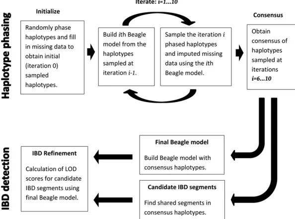
Overview of the Reﬁned IBD algorithm

Figure 1 gives an overview of the Refined IBD algorithm. The first part of the algorithm (top row in Figure 1) estimates haplotype phase. Subsequent to haplotype phase determina-tion, there are two steps in the Refined IBD algorithm (bot-tom row in Figure 1). Thefirst is identification of candidate IBD segments. The candidate segments are regions in which two individuals share an identical statistically phased hap-lotype segment that is longer than a specified threshold. In the second step, we use the phased haplotypes to build a haplotype frequency model, and for each candidate IBD segment we calculate the likelihood of an IBD model (one haplotype shared IBD) and of a non-IBD model (no haplo-types shared IBD). We compute the LOD score, which is the base 10 log of the likelihood ratio. Candidate segments hav-ing LOD score greater than a specified threshold (the default threshold is 3.0) are reported as IBD segments.

It is possible to run Reﬁned IBD several times with different random-number seeds and to merge the resulting IBD seg-ments. Except as otherwise noted, all results presented here

are from a single run. IBD segments from multiple runs for a sample pair are combined by taking the union of the IBD segments from the multiple runs and merging overlapping IBD segments in the union. Merging is performed sequentially on pairs of overlapping segments. Whenever a pair of overlapping segments is found, the pair of IBD segments is replaced with the merged IBD segment. The merged IBD segment’s chromo-some interval is the union of the overlapping intervals, and the merged segment’s LOD score is the maximum LOD score of the overlapping intervals. Merging IBD segments from multi-ple runs results in greater power to detect long IBD segments at the cost of increased run time and loss of haplotype information.

Refined IBD reports the index (1 or 2) of the IBD haplotype in each individual. Each index identifies one of the two ordered consensus haplotypes of an individual that are reported by Beagle. However, when IBD segments from multiple runs are merged, the haplotype identification is lost as the estimated haplotype phase typically differs slightly between runs.

Identiﬁcation of candidate IBD segments

When applying the GERMLINE algorithm to detect candi-date IBD segments, we do not permit any mismatching alleles in the shared haplotype. Each candidate IBD segment is deﬁned by its starting and ending genome coordinates, the pair of sample identiﬁers, and the haplotype index (1 or 2) of the shared haplotype for each sample.

The ibdwindow parameter in Beagle version 4 deter-mines the number of markers included in each window when using the GERMLINE algorithm toﬁnd candidate IBD segments. The ibdwindow parameter is equivalent to the GERMLINE bits parameter. Too large a value may result in missing short segments of IBD, while too small a value will increase computation time. The default value of 64 is suitable for SNP arrays with 1 million SNPs across the genome, as at this marker density, 64 markers correspond to 0.2 cM, which is signiﬁcantly shorter than the default threshold on IBD segment length. For SNP array data, we recommend setting this parameter to approximately the average number of markers per 0.2 cM.

The ibdcm parameter in Beagle version 4 controls the minimum genetic length of a candidate IBD segment. A value that is too small will result in increased computing time while not contributing much to IBD detection as small candidate segments are unlikely to pass the LOD score threshold. The default value of 1.0 cM was chosen based on the relatively low power to detect smaller segments in SNP array data (see

Results).

Haplotype frequency models for IBD and non-IBD

(3)

Browning 2009). We calculate the probability of the observed genotype data for a pair of individuals under a non-IBD model (the likelihood of non-IBD), using the HMM for un-related individuals, and we calculate the probability of the observed genotype data for a pair of individuals under an IBD model (the likelihood of IBD), using the HMM for a parent– offspring pair since a parent–offspring pair also shares one haplotype identical by descent.

A HMM is deﬁned by its state space, initial probabilities, transition probabilities, set of emitted symbols, and emission probabilities (Rabiner 1989). Since the Beagle HMMs for unrelated individuals and parent–offspring pairs have been fully described previously (S. R. Browning and B. L. Brown-ing 2007, 2009), we give only a brief description of these HMMs here. In the Beagle HMM, there is a set of haploid hidden states Sm corresponding to each marker m. Each haploid hidden state corresponds to a cluster of haplotypes that are locally similar around marker m. The hidden state for a diploid individual at markermis an elementðs1;s2Þ 2S2m, wheres1 is the state of theﬁrst haplotype, ands2 is the state

of the second haplotype of the individual. The hidden state of a parent–offspring pair at marker m is an element ðs1;s2;s3Þ 2S3m, whereðs1;s2Þis the hidden state of the

par-ent,ðs1;s3Þis the hidden state of the offspring, ands1 is the

hidden state of the shared haplotype.

In the Beagle HMM, each haploid hidden state at marker

mis labeled with one of the marker’s alleles (more than one hidden state at marker m can be labeled with the same allele). The emission probability for the labeled allele is 1, while the emission probability for any other allele is 0. For parent–offspring pairs, this means that the probability of the observed genotypes given the hidden stateðs1;s2;s3Þ 2S3mis 1 if the alleles labeling s1 and s2 are consistent with the

observed genotype of the parent at markermand the alleles labelings1ands3are consistent with the observed genotype

of the offspring at markerm; the probability is 0 otherwise.

Each haplotype used to build the Beagle HMM has a unique path through the model. Thus each haploid state has an associated count of how many haplotypes pass through the state, and similarly each possible transition has an associated count. Consider a haploid transition in the Beagle HMM. Call the state that the transition starts from at markermthe “source”state and the state that the transition goes to at markermþ1 the“destination”state. The transition proba-bility is the count associated with that transition divided by the count associated with the source state for the transition. In other words, of those haplotypes passing through the source state, the transition probability is the proportion that transitions into the destination state. Given a starting markerm, the initial probability for a haploid state at marker

mis equal to the proportion of haplotypes that pass through that state, which is the count associated with that state di-vided by the total number of haplotypes used to build the model. Transition and initial probabilities for unrelated dip-loid individuals (pairs of hidden states) or parent–offspring pairs (triples of hidden states) are obtained by multiplying the corresponding haploid probabilities.

Since IBD segments are typically much shorter than their corresponding chromosome, we reduce computation time by calculating likelihoods using only genotype data in the interior of the candidate IBD segment. In this way, we can also avoid modeling the recent recombination events that demarcate the boundaries of the IBD segment. It is difﬁcult to identify the IBD segment endpoints with high accuracy. Incorrectly including some non-IBD markers at the ends of a real IBD segment can result in a severely reduced LOD score for the segment, while incorrectly removing small parts of the ends of a real IBD segment tends to result in only a small drop in LOD score. We thus trim a smallﬁxed number of markers from each end of the candidate IBD segment and compute likelihoods of the non-IBD and IBD models in the trimmed genomic interval. The trimmed markers are restored to the

(4)

IBD segment after calculation of the likelihoods. The number of markers to trim when calculating the LOD score is con-trolled by the ibdtrim parameter in Beagle version 4. In-creasing the trim number will reduce power to detect short segments. When a short candidate segment is trimmed there may not be enough markers left to provide sufﬁcient in-formation to be conﬁdent of IBD. The default trim value (40) was chosen based on analyses of the Wellcome Trust Case Control Consortium 2 data, by looking for a value that would maximize the amount of IBD detected (data not shown). For SNP array data we recommend setting the trim value to approximately the average number of markers per 0.15 cM.

The likelihoods for the IBD and non-IBD models are calculated using Baum’s forward algorithm (Baum 1972). For the non-IBD model, the probability of the observed data for a pair of individuals is the product of the probabilities for each individual.

Other improvements to Beagle in version 4

As well as implementing Reﬁned IBD, Beagle version 4 has improvements to haplotype phasing and to general usability. Beagle version 4 reports the consensus haplotype for each individual. Other haplotype phasing programs also use consensus haplotypes (Scheet and Stephens 2006; Li et al.

2010). Previous versions of Beagle have used the Viterbi algorithm (Viterbi 1967) to generate the reported phased haplotypes. However, we have found the consensus haplo-types to be more accurate than the haplohaplo-types obtained from the Viterbi algorithm.

For consensus haplotypes, haplotypes are estimated at multiple iterations (or from multiple runs) of the phasing algorithm, and the results are merged. The top row of Figure 1 illustrates the procedure for obtaining consensus haplo-types in Beagle version 4. The haplotype phasing module involves multiple iterations of estimating (sampling) haplo-types based on a provisional model and then updating the model based on the new estimated haplotypes. By default, four pairs of haplotypes are sampled per individual per iter-ation. Haplotypes estimated in thefirst few iterations are not likely to be very accurate, because the provisional model is still in the initial stages of converging toward a good solu-tion. Thus, in Beagle version 4, the consensus haplotypes are obtained from all sampled haplotypes after a specified num-ber of burn-in iterations (five burn-in iterations and five additional iterations by default). Under default settings there are 20 pairs of sampled haplotypes per individual that are used for obtaining the consensus haplotypes (4 pairs per iteration·5 iterations after burn-in).

Theﬁrst step in obtaining the consensus haplotypes is to obtain consensus genotypes for those genotypes that were missing. Consensus genotypes are obtained by taking the most frequently sampled genotype, breaking ties randomly. After consensus genotypes are obtained, the consensus phasing for an individual is obtained by working along the chromosome, one pair of successive heterozygous genotypes at a time. A pair of successive heterozygous genotypes has

no intervening heterozygous genotypes. Only sampled hap-lotype pairs having the consensus heterozygous genotype at both markers are used to determine the consensus phasing. The consensus phasing of two successive heterozygous ge-notypes is determined by majority vote, breaking ties ran-domly. For example, in phasing the genotypes AC and TG, if 16 sampled haplotype pairs have AT/CG phase, while 4 sampled haplotype pairs have AG/CT phase, the consensus haplotypes will have the AT/CG phase.

Beagle version 4 uses Variant Call Format for input and output dataﬁles (Daneceket al.2011). Variant Call Format is a standard, widely used format for genotype data (1000 Genomes Consortium 2010), and use of this format will re-duce the need for tedious dataﬁle format conversion.

Beagle version 4 also uses a sliding marker window that makes the memory usage independent of the number of markers in the data set. Decreased accuracy near the edge of the marker windows is avoided by using overlapping win-dows and trimming half of the overlap from each window prior to merging data in adjacent windows. Haplotypes in adjacent marker windows are aligned using a heterozygote near the middle of the overlap.

Scale factors

The Beagle HMM is represented by a directed acyclic graph. When the model is constructed, a process of node merging occurs. Two nodes of the graph, xandy, are merged if the maximum difference in downstream frequencies is less than a threshold (B. L. Browning and S. R. Browning 2007). The threshold is

mðn21x þny21Þ1=2þb; (1)

wheremis the scale factor,bis the shift parameter, andnx andnyare the numbers of haplotypes whose path through the graph includes nodes x and y, respectively. The scale and shift parameters were originally introduced to control the degree of parsimony of the ﬁtted Beagle model when performing association testing (B. L. Browning and S. R. Browning 2007). Larger values of these parameters result in more merging of nodes and hence a more parsimonious model. Without the added parsimony, each haplotype clus-ter may contain very few observations, reducing power to detect an association.

(5)

values $2 is somewhat arbitrary, provided that appropriate compensatory adjustment is made to the threshold for signifi -cance of the fastIBD score or the Refined IBD LOD score (data not shown). However, as the sample size changes, the optimal choice of IBD scale factor for afixed score threshold changes. For a given choice of IBD scale parameter, as more individuals are added to the data, the fitted model becomes larger (less parsimonious). A larger model allows for higher precision in haplotype frequency estimation, resulting in fewer false posi-tives. On the other hand, the requirement that shared haplo-types must traverse the same path through the model to be declared IBD becomes more onerous as the model size increases, and detection rates can drop.

Therefore, to have a single LOD score threshold regard-less of sample size, the IBD scale factor must increase as the sample size increases and the size (complexity) of thefitted Beagle model must stay approximately constant, to maintain power to detect IBD as sample size increases. Since model complexity is controlled by the merging threshold given in Equation 1, when the sample size increases by a factor ofk, the IBD scale factor can be increased by a factor of pffiffiffik to keep the typical threshold at approximately the same level, resulting in a similar size of model. We chose to make the default setting for the IBD scale factorpffiffiffiffiffiffiffiffiffiffiffiffiffiffin=100, when the sample size,n, is.400. This results in IBD scale factors of 2.2 for 500 samples, 4.5 for 2000 samples, and 7.1 for 5000 samples. For sample sizes,400, we set the default IBD scale factor to 2, as decreasing the IBD scale factor below 2 can reduce power to find IBD.

In summary, with reference to Equation 1 and Figure 1, a scale factor of 1 is used for model building during haplo-type phasing (top row of Figure 1). However, an IBD scale factor.1 is used for building theﬁnal Beagle model for IBD reﬁnement (bottom row of Figure 1), as described above. A shift of 0 is used in all cases.

Simulated SNP data

To assess false positive and true positive IBD detection rates, we simulated data. In our simulation data, we attempted to match both current and historical effective population sizes, to obtain a good match with real data. Ancient historical population sizes affect the number of common variants and the extent of LD between them. The extent of LD affects power to detect IBD and can affect false positive IBD detection rates. Current and very recent population sizes affect the number of rare variants and the amount of detectable IBD. The amount of detectable IBD in the simulation is critical. Our method is designed for large outbred populations in which the amount of detectable IBD is low, so we want the simulated data to reﬂect this.

Recent analyses of the allele frequency spectrum, with particular attention paid to the rare end of the spectrum, have shown that explosive population growth has occurred in the past few hundred generations (Keinan and Clark 2012). In our view, previous modelsﬁtted to sequence data do not go far enough in modeling this growth, as they allow

only for a single rate of recent growth, resulting in growth rate estimates of 2% (Nelson et al.2012) or 9% (Coventry

et al. 2010) per generation. In contrast, census data show that the rate of population growth has accelerated in the past few hundred generations and is currently 30% per generation globally (Keinan and Clark 2012).

We used Fastsimcoal (Excofﬁer and Foll 2011) to simu-late sequence data that we then thinned to obtain simusimu-lated SNP array data. We simulated 10 regions, each with 30 Mb of sequence on 2000 diploid individuals. We used a mutation rate of 2.5·1028_{(Nachman and Crowell 2000) and a}

re-combination rate of 1028₍_i.e._{, 1 Mb = 1 cM). Our}

simula-tion scheme was designed with European populasimula-tions in mind, as our available real data are from European pop-ulations. The effective population size was initially (prior to expansion beginning 300 generations ago) 3000 diploid individuals. This reﬂects the European effective population size estimated using LD between common variants (Tenesa

et al.2007). In our simulations, the effective population size began to grow 300 generations ago (timing reflects the ad-vent of large-scale organized agriculture) at a rate of 1.8% per generation (reflecting, e.g., the 1.7% growth rate esti-mate in Nelsonet al.2012), reaching 270,000 by 50 gener-ations ago. We modeled population growth rate increases in the past 50 generations based on English census data, as shown in Supporting Information,Figure S1. At 50 gener-ations ago, we increased the growth rate to 5%, giving ef-fective population size 2 million at 10 generations ago. We increased the growth rate further, to 25% per generation, for the final 10 generations, yielding an effective population size of 24 million ð2·106_·_expð0_:₂₅_·_10ÞÞ _{at the current}

generation.

After generating the sequence data, we created simulated SNP array data from it by removing all variants with more than two alleles and all variants with frequency ,2%, and by selecting variants from those remaining to obtain1000 variants per 30-Mb region (corresponding to a SNP density of 1 million SNPs genome-wide) with minor allele frequen-cies uniformly distributed between 2% and 50%. We then added genotype error at a rate of 0.05%, reﬂecting the very high accuracy seen in current genotyping arrays after apply-ing standard quality control ﬁlters (Steemers et al. 2006). Genotype error was introduced by converting homozygote genotypes to heterozygote and by converting heterozygote genotypes to a randomly chosen homozygote genotype. We also removed haplotype phase information.

(6)

different random-number seeds and merged the results. We ran Beagle IBD (Beagle version 3.3.1) (Browning and Browning 2010) with 10 different random-number seeds, with the default IBD scale of 2 for 500 individuals. We did not run Beagle IBD with all 2000 individuals due to its long computing times.

We ran GERMLINE version 1.5.1 (Gusevet al.2009) with parameters used in Gusevet al.(2011). Speciﬁcally, we used options“-haploid -min_m 1 -bits 32 -err_hom 1 -err_het 1”. The“-min_m 1”option means that GERMLINE reports only IBD segments with estimated length$1 cM. The“-haploid” option ensures that GERMLINE makes use of the haplotype phase information. Our previous published analyses with GERMLINE used GERMLINE’s default setting that does not use haplotype phase information (B. L. Browning and S. R. Browning 2010, 2011). As seen by comparing the results presented here with the results in our earlier work,

utili-zation of haplotype phase information greatly improves GERMLINE’s performance on SNP array data. We used the phased haplotypes output from the Beagle Reﬁned IBD anal-ysis as input to GERMLINE. These haplotypes are based on a consensus of haplotypes sampled at different iterations of the Beagle phasing algorithm, as described above, and have accuracy higher than that from previous versions of Beagle run with default settings. The high SNP density (equivalent to a SNP array with 1 million SNPs) also contributes to high phasing accuracy. The high accuracy of these haplotypes facil-itates the strong performance of GERMLINE in these data.

We used the full simulated phase-known sequence data to determine the true IBD status, so that we could assess the accuracy of the IBD estimated from the thinned, phase-agnostic SNP data. When determining the true IBD, we ignored variants with#10 copies in the 2000 individuals, as very recent mutations disrupt sequence identity. For two IBD

(7)

haplotypes separated bymmeioses, looking along the chro-mosome, recombination ends the IBD at rate m times the recombination rate, while new mutations disrupt the se-quence identity at rate mtimes the mutation rate. In our simulation, the mutation rate is 2.5 times the recombination rate, so in any IBD segment we expect an average of 2.5 identity-disrupting new mutations. Ignoring variants with

#10 copies, we declared pairs of haplotypes with identical sequence for at least 0.1 cM to be segments of true IBD for the purpose of assessing IBD detection accuracy.

Simulated sequence data

Using the simulated phased sequence data described above, we also created simulatedﬁltered, unphased sequence data with genotype errors. We removed variants with more than two alleles or with minor allele frequency ,0.5%, added genotype error at a rate of 0.1%, and removed information

about genotype phase. The minor allele frequency filter of 0.5% was chosen to be higher than the threshold used to determine true IBD (0.25%). This allows the variants with frequency in the 0.25–0.5% range to be used to assess ac-curacy of the detected IBD segments. Error rates in sequence data vary considerably, depending on the depth of sequence coverage. We chose to use a per-variant error rate twice that of the simulated SNP data. The number of genotype errors occurring in an IBD segment is also increased in sequence data since there are more variants and thus more opportunities for error. We analyzed 500 individuals of the simulated unphased filtered sequence data, using Refined IBD with a minimum segment length of 0.2 cM and LOD scores of 4 and 5.

Wellcome Trust Case Control Consortium 2 data

The Wellcome Trust Case Control Consortium phase 2 con-trols consist of 5200 individuals from the United Kingdom

(8)

genotyped on a custom Illumina array (Barrett et al.2009). After quality control, including removal of SNPs not in Hardy–Weinberg equilibrium (P,1025_{) and SNPs with}

mi-nor allele frequency,1%, 885,127 autosomal SNPs remained for analysis. We ran Reﬁned IBD with a minimum genetic length threshold of 0.5 cM. We used windows of 10,000 markers (window = 10,000) with 1000-marker overlap be-tween adjacent windows (overlap = 1000). Other parameters were left at their default values. Genetic lengths of detected IBD segments in these data and in the Finnish data (described below) were determined using the estimated genetic distances provided by the International Haplotype Map Consortium (Frazeret al.2007).

Northern Finland Birth Cohort data

The Northern Finland Birth Cohort data consist of 5402 individuals from Northern Finland, born in 1966, with geno-types on 320,981 autosomal SNPs from an Illumina Infinium SNP array (Sabatti et al.2009). We excluded 503 individuals with close relatives (relatedness equivalent to first cousins or closer) in the data, as described previously (Browning and Browning 2013), leaving 4899 individuals for analysis. Due to the relatively low density of SNPs in these data, we used a smaller number of SNPs for the IBD detection windows in the GERMLINE algorithm (ibdwindow = 32) and a smaller than usual trim for the likelihood-ratio score (ibdtrim = 30). To reduce memory requirements, we took advantage of the windowing built into Beagle 4 and used 2000 marker win-dows (20 Mb) with a 400-marker overlap between adja-cent windows (4 Mb). Other parameters for Refined IBD were left at their default values.

Results

Simulation study

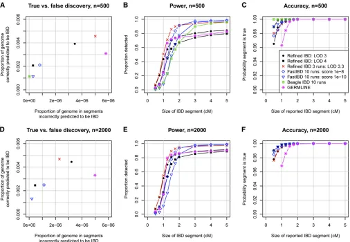
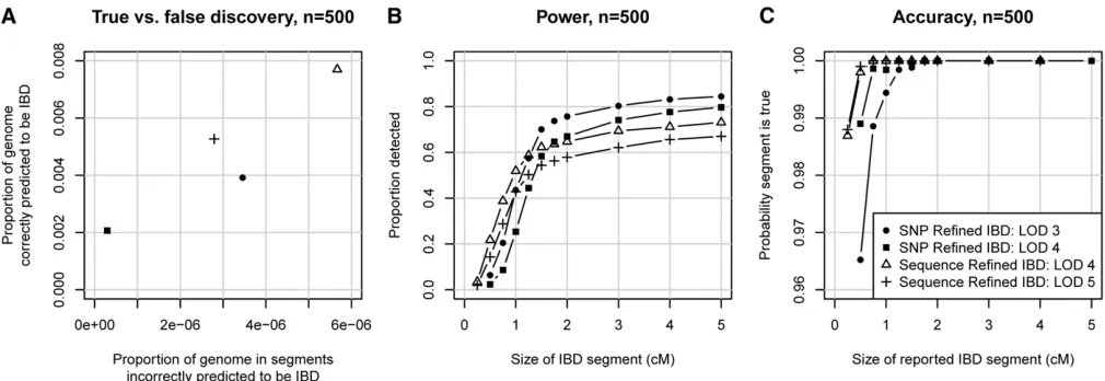
To compare the proposed Refined IBD method with existing methods, we generated simulated SNP data (seeMethods) on ten 30-Mb regions, with 500 and with 2000 simulated individuals. Figure 2 summarizes the accuracy of the meth-ods. Figure 2, A and D, shows that Refined IBD with LOD score threshold 3 has higher accuracy and higher power than GERMLINE. Figure 2, B, C, E, and F, shows that Re-fined IBD has higher power than fastIBD to detect short (,1–2 cM) IBD segments for comparable levels of accuracy. In contrast, fastIBD has better ability to detect close to 100% of the larger segments (.2 cM) whereas Refined IBD typi-cally misses 10–20% of these larger segments. FastIBD does a good job of not missing parts of large segments because the algorithm is run 10 times, so that phasing errors in one run may be avoided in a different run. When we ran Refined IBD 3 times with different random-number seeds and merged the results, much of the missed IBD was recovered (Figure 2). Similar results can be obtained with less compu-tation by joining high-confidence IBD segments with nearby low-confidence segments from a single run of Refined IBD

(data not shown). Overall accuracy for all the methods con-sidered here is very high, with at least 94% of reported segments reﬂecting true underlying IBD. For several of the methods, depending on parameter settings, power is high to detect segments of size$1 cM, particularly when the larger sample size is used.

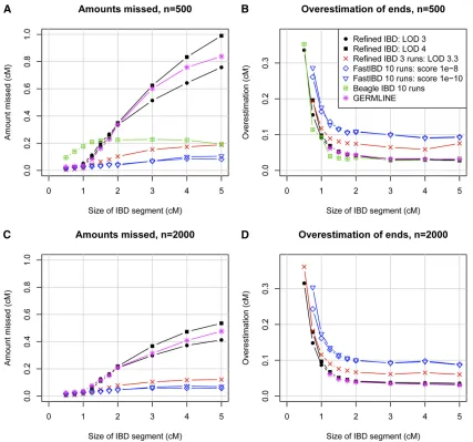
The most challenging part of IBD detection is determi-nation of the IBD endpoints. Inferred haplotype allele identity may extend beyond the true IBD region, leading to overestimation of IBD endpoints. Furthermore, determina-tion of haplotype phase is difficult at the IBD endpoints because the recent recombination demarcating the IBD endpoints disrupts the haplotypes, and consequent phase errors lead to incorrect determination of IBD endpoints. In Figure 2, we classified a reported IBD segment as true or false by whether it at least partly reflected some underlying IBD. This approach was designed to avoid conflating accuracy at the boundaries of the reported segment with accuracy of the segment itself. In Figure 3, we consider under- and over-estimation of the IBD segment. Both types of error are pri-marily due to incorrect determination of segment endpoints. Overestimation is always on the ends of an IBD segment, while underestimation can occur in the middle of an IBD segment (if two or more short segments are reported, with intervening gaps, instead of one long segment) as well as at the ends. It can be seen that fastIBD with the recommended 10 iterations tends to significantly overestimate endpoints

(9)

and misses very little of the true underlying segments when the segments are at least partly found. In contrast, GERMLINE and Reﬁned IBD have much less overestimation of endpoints, but tend to miss large parts of the segment. Reﬁned IBD with three runs is almost as good as fastIBD with respect to underestimation and is better than fastIBD with respect to overestimation. It also has a better true vs.

false discovery profile than fastIBD due to better ability to detect short segments (Figure 2). Refined IBD with a single run misses much less IBD from longer segments with a sam-ple size of 2000 individuals than with a samsam-ple size of 500 individuals. This is probably because haplotype phase esti-mation accuracy increases with sample size (S. R. Browning and B. L. Browning 2007), and increased haplotype phase accuracy increases the ability tofind most or all of a larger IBD segment.

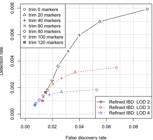
Depending on the application, one may wish to be conservative in reporting the IBD segment endpoints. One approach is to trim aﬁxed number of markers from each end of the detected segments. Figure 4 shows how the accuracy (including overestimation and falsely detected segments) and the true IBD detection rate vary by LOD score threshold and amount trimmed. The optimal combination depends on the level of accuracy required. For higher detection at the cost of lower accuracy, a less stringent LOD score threshold such as 2 combined with a light to moderate level of trim-ming (up to 100 markers) is best. For high accuracy, such as a false discovery rate,1%, one needs a stringent LOD score threshold such as 4 combined with a high level of trimming ($100 markers). A high level of trimming both removes potential overestimation from the detected segments and removes short segments that are slightly less likely to reﬂect true underlying IBD (Figure 2, C and F).

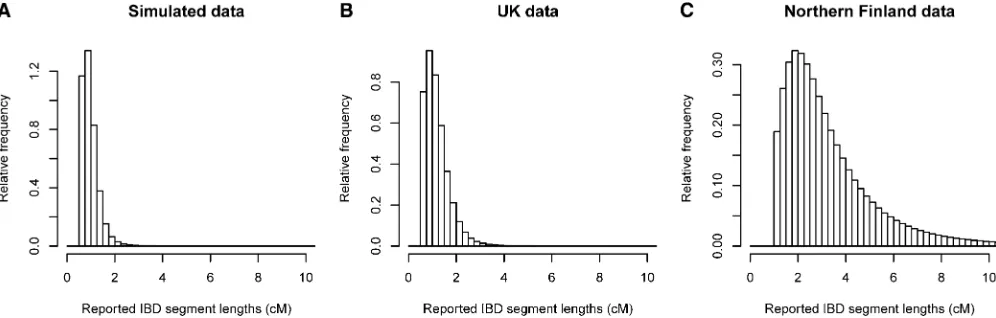
When using a LOD score threshold of 3 (to match the threshold used in the United Kingdom and Finnish data analyses), we found IBD at a rate of 0.0043. (The IBD detection rate is the probability that a randomly chosen pair of individuals has detectable IBD at a randomly chosen position.) The distribution of IBD segment lengths is shown

in Figure 5A. Overall, the simulated data have a slightly higher rate of IBD detection and a somewhat lower average IBD segment size compared to the United Kingdom data (see United Kingdom results below).

In the results described above, the rate of genotype error was very low (0.05%), which reflects the high level of accuracy that can be achieved with quality-control–filtered SNP array data. InFigure S2, we investigate the effects of a higher rate of error (0.5%) on IBD segment detection with Refined IBD. We find that increasing the genotype error rate does not adversely decrease accuracy, but does decrease power to detect IBD.

Simulated sequence data

We generated simulated sequence data on 500 individuals. For the Reﬁned IBD analysis, we excluded all variants with minor allele frequency #0.5% and added genotype error at a rate of 0.1%, which is twice that of the SNP data. Figure 6 compares IBD detection results for the simulated sequence data with those for the simulated SNP data. In the sequence data we found we needed to use a higher LOD score threshold than in SNP data to control false IBD seg-ment discovery to a similar level. However, it should be noted that the overall level of reported segments is much higher in the sequence data, so the ratio of false to true discoveries is still well controlled with a LOD score of 3. For the same false positive IBD detection level, we detect 50% more true IBD in the sequence data (Figure 6A). Figure 6B shows that the increase in power is due to in-creased ability to detect segments ,1 cM. On the other hand, some of the IBD in segments.2 cM is being missed. One reason for the missed parts of long segments is the higher level of genotype error, due to both a higher error rate per variant and a higher density of variants. The phasing of the sequence data may also have a higher number of switch errors per centimorgan because low-frequency variants are generally more difﬁcult to phase than high-frequency variants. Figure 6C shows that the accuracy of the IBD segments detected from the simulated sequence data is very high, even for segments as short as 0.25 cM.

(10)

Wellcome Trust Case Control Consortium 2 data

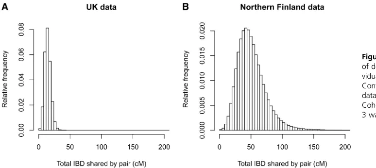
We analyzed900,000 autosomal SNPs genotyped on 5200 individuals from the United Kingdom. The average amount of IBD detected on the autosomes was 14.4 cM per pair of individuals. This equates to an IBD detection rate of 0.0041. Only 224 pairs (0.0017% of pairs) had no detected IBD. Figure 5B shows the distribution of detected IBD lengths, while Figure 7A shows the distribution of the amount of detected IBD per pair of individuals.

Northern Finland Birth Cohort data

We analyzed300,000 autosomal SNPs genotyped on 4899 individuals from Northern Finland after excluding close rel-atives. The average amount of IBD detected on the auto-somes was 51.5 cM per pair of individuals. This equates to an IBD detection rate of 0.015, which is 3.6 times as high as that in the United Kingdom data, even though the United Kingdom data have much higher SNP density and thus much better power to detect small IBD segments. Only 675 pairs (0.0056% of pairs) had no detected IBD. Figure 5C shows the distribution of detected IBD lengths, while Figure 7B shows the distribution of the amount of detected IBD per pair of individuals.

Computation time

Computing requirements for IBD detection with Reﬁned IBD are the same order of magnitude as the Beagle phasing time for the data sets we analyzed, although the actual IBD de-tection time depends on the amount of IBD found in the data, which in turn depends on the minimum IBD length parameter, the SNP density, the effective size of the popula-tion from which the sample was drawn, and the sample size. For example, in the United Kingdom data on chromosome 1, phasing took 78 hr while IBD detection took 94 hr with a minimum IBD length parameter of 0.5 cM. In the Northern Finland data on chromosome 1, phasing took 28 hr while IBD detection took 55 hr with a minimum IBD length parameter

of 1.0 cM. In the simulated SNP data with 2000 individuals on 30 Mb, phasing took 113 min while IBD detection took 158 min with a minimum IBD length parameter of 0.5 cM. In simulated SNP data with 500 individuals on 30 Mb, phasing took 10 min while IBD detection took 7 min. In simulated sequence data with 500 individuals on 30 Mb, phasing took 68 min while IBD detection took 70 min with a minimum IBD length parameter of 0.2 cM. All computation times are from runs on a 2.4-GHz computer.

In general, computation time scales linearly with the chro-mosome length and quadratically in the number of individ-uals. Candidate IBD segments are efﬁciently identiﬁed using the GERMLINE hashing algorithm (Gusevet al.2009), while calculation of LOD scores is linear in the number of candidate segments and hence quadratic in the number of individuals.

Discussion

In our simulated SNP data, Refined IBD has significantly higher power than existing computationally efficient IBD detection methods while maintaining the same high level of accuracy. The gain in power is seen primarily in the smaller segment sizes, such as 0.5–1 cM. This makes Refined IBD useful for analyses in outbred populations, in which there are few long IBD segments but many short IBD segments. The additional detected short IBD segments will improve the power of IBD mapping (Browning and Thompson 2012), facilitate haplotype phasing in population samples (Kong

et al. 2008), and permit higher resolution when estimating population structure (Gusev et al. 2012; Palamara et al.

2012).

When accurate detection of long (e.g.,.3 cM) segments of IBD is required, we recommend merging results from multiple runs of Refined IBD andfilling any short (e.g.,,2 cM) gaps between IBD segments. This approach greatly increases power to find the complete long segment of IBD, but can result in a small amount of overestimation of the length of the segment (see Figure 3).

(11)

Our analysis of simulated sequence data shows that Re-ﬁned IBD can be used for IBD detection in sequence data. However, further development of IBD detection methodology for sequence data is needed. Such methods should be designed to take full advantage of the information contained in rare variants while accounting for both the higher ge-notype error rate in sequence data and the possibility of mutations occurring in an IBD segment since the common ancestor.

Our analysis of data from United Kingdom individuals found significantly more IBD than a previous study. Here we found IBD at a rate of 0.0041 (probability that a randomly chosen pair of individuals has detectable IBD at a randomly chosen position), whereas the previous rate was 0.00035 (B. L. Browning and S. R. Browning 2011). This difference is due in part to the improved sensitivity of Refined IBD over that of fastIBD (see Figure 2). An even more significant contributing factor is the relative SNP densities in the two anal-yses. The earlier analysis was of500,000 SNPs genome-wide, while the analysis presented here uses almost twice as many SNPs. At higher SNP densities, power to detect small seg-ments increases. While small segseg-ments individually contrib-ute little IBD, there are many more small segments than large, since the number of ancestors of an individual can increase exponentially with the number of generations to the ancestors. Thus SNP density can have a large effect on the rate of IBD detected.

Compared to the United Kingdom data, the Northern Finland data show a much higher rate of detected IBD (0.015vs.0.0041). This high level of IBD is to be expected in an isolated population. A high level of detected IBD enables the application of IBD-based heritability estimation. In pre-vious IBD-based heritability analysis of these data, we found signiﬁcant heritability for cholesterol and fasting glucose levels (Browning and Browning 2013).

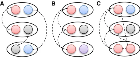
The haplotype-based output of Reﬁned IBD is useful for downstream analyses. In individual-based IBD detection, one does not know whether three individuals who are all IBD with each other are IBD for the same haplotype or not, as illustrated in Figure 8. A previous approach to the

multi-individual IBD problem was joint analysis of multiple indi-viduals (Moltkeet al.2011); however, this is computationally demanding. With haplotype-based IBD, there is some uncer-tainty in determining the multi-individual haplotype IBD be-cause some IBD is not detected, while false positive IBD can occur. Gusevet al.(2011) apply clustering to deal with this issue. With determination of multi-individual IBD, it becomes possible to extend IBD mapping from the existing pairwise approaches (Purcell et al. 2007; Browning and Thompson 2012) to a multi-individual approach (Gusev et al. 2011), potentially making better use of the information in the data. Another advantage of haplotype-based output is that one can directly match the haplotypes to the IBD, so that if oneﬁnds an interesting pattern of IBD sharing, one can identify the underlying shared haplotypes.

Web resources

The Beagle webpage ishttp://faculty.washington.edu/browning/ beagle/beagle.htmlVariant call format speciﬁcation:http:// vcftools.sourceforge.net/specs.html.

Acknowledgments

The Northern Finland Birth Cohort (NFBC1966) Study is conducted and supported by the National Heart, Lung, and Blood Institute (NHLBI) in collaboration with the Broad Institute, University of California at Los Angeles (UCLA), University of Oulu, and the National Institute for Health and Welfare in Finland. This article does not necessarily reﬂect the opinions or views of the NFBC1966 Study Investigators, Broad Institute, UCLA, University of Oulu, the National Institute for Health and Welfare in Finland, and the NHLBI. This study makes use of data generated by the Wellcome Trust Case Control Consortium. A full list of the investi-gators who contributed to the generation of the data is available from www.wtccc.org.uk. Funding for the project was provided by the Wellcome Trust under awards 076113 and 085475. This study was supported by research grants HG004960, HG005701, GM099568, and GM075091 from the National Institutes of Health.

(12)

Literature Cited

1000 Genomes Consortium, 2010 A map of human genome var-iation from population-scale sequencing. Nature 467: 1061– 1073.

Albrechtsen, A., T. S. Korneliussen, I. Moltle, T. V. Hansen, F. C. Nielsenet al., 2009 Relatedness mapping and tracts of relat-edness for genome-wide data in the presence of linkage disequi-librium. Genet. Epidemiol. 33: 266_–274.

Barrett, J. C., J. C. Lee, C. W. Lees, N. J. Prescott, C. A. Anderson

et al., 2009 Genome-wide association study of ulcerative co-litis identi_ﬁes three new susceptibility loci, including the HNF4A region. Nat. Genet. 41: 1330–1334.

Baum, L. E., 1972 An inequality and associated maximization technique in statistical estimation for probabilistic functions of Markov processes, pp. 1–8 inInequalities III: Proceedings of the Third Symposium on Inequalities held at the University of Califor-nia,Los Angeles,September 1–9,1969, edited by O. Shisha. Ac-ademic Press, San Diego.

Brown, M. D., C. G. Glazner, C. Zheng, and E. A. Thompson, 2012 Inferring coancestry in population samples in the pres-ence of linkage disequilibrium. Genetics 190: 1447–1460. Browning, B. L., and S. R. Browning, 2007 Efﬁcient multilocus

association testing for whole genome association studies using localized haplotype clustering. Genet. Epidemiol. 31: 365_–375. Browning, B. L., and S. R. Browning, 2009 A uni_ﬁed approach to genotype imputation and haplotype-phase inference for large data sets of trios and unrelated individuals. Am. J. Hum. Genet. 84: 210_–223.

Browning, B. L., and S. R. Browning, 2011 A fast, powerful method for detecting identity by descent. Am. J. Hum. Genet. 88: 173–182.

Browning, S. R., and B. L. Browning, 2007 Rapid and accurate haplotype phasing and missing-data inference for whole-genome association studies by use of localized haplotype clus-tering. Am. J. Hum. Genet. 81: 1084–1097.

Browning, S. R., and B. L. Browning, 2010 High-resolution de-tection of identity by descent in unrelated individuals. Am. J. Hum. Genet. 86: 526–539.

Browning, S. R., and B. L. Browning, 2011 Haplotype phasing: exist-ing methods and new developments. Nat. Rev. Genet. 12: 703–714. Browning, S. R., and B. L. Browning, 2012 Identity by descent between distant relatives: detection and applications. Annu. Rev. Genet. 46: 617_–633.

Browning, S. R., and B. L. Browning, 2013 Identity-by-descent-based heritability analysis in the Northern Finland Birth Cohort. Hum. Genet. 132: 129–138.

Browning, S. R., and E. A. Thompson, 2012 Detecting rare variant associations by identity-by-descent mapping in case-control studies. Genetics 190: 1521–1531.

Cai, Z., N. J. Camp, L. Cannon-Albright, and A. Thomas, 2011 Identiﬁcation of regions of positive selection using Shared Genomic Segment analysis. Eur. J. Hum. Genet. 19: 667–671.

Campbell, C. L., P. F. Palamara, M. Dubrovsky, L. R. Botigue, M. Fellouset al., 2012 North African Jewish and non-Jewish pop-ulations form distinctive, orthogonal clusters. Proc. Natl. Acad. Sci. USA 109: 13865_–13870.

Coventry, A., L. M. Bull-Otterson, X. Liu, A. G. Clark, T. J. Maxwell

et al., 2010 Deep resequencing reveals excess rare recent var-iants consistent with explosive population growth. Nat. Com-mun. 1: 131.

Danecek, P., A. Auton, G. Abecasis, C. A. Albers, E. Banks et al., 2011 The variant call format and VCFtools. Bioinformatics 27: 2156–2158.

Excofﬁer, L., and M. Foll, 2011 fastsimcoal: a continuous-time coalescent simulator of genomic diversity under arbitrarily com-plex evolutionary scenarios. Bioinformatics 27: 1332–1334. Frazer, K. A., D. G. Ballinger, D. R. Cox, D. A. Hinds, L. L. Stuve

et al., 2007 A second generation human haplotype map of over 3.1 million SNPs. Nature 449: 851–861.

Gusev, A., J. K. Lowe, M. Stoffel, M. J. Daly, D. Altshuler et al., 2009 Whole population, genome-wide mapping of hidden re-latedness. Genome Res. 19: 318_–326.

Gusev, A., E. E. Kenny, J. K. Lowe, J. Salit, R. Saxena et al., 2011 DASH: a method for identical-by-descent haplotype mapping uncovers association with recent variation. Am. J. Hum. Genet. 88: 706–717.

Gusev, A., P. F. Palamara, G. Aponte, Z. Zhuang, A. Darvasiet al., 2012 The architecture of long-range haplotypes shared within and across populations. Mol. Biol. Evol. 29: 473–486.

Han, L., and M. Abney, 2011 Identity by descent estimation with dense genome-wide genotype data. Genet. Epidemiol. 35: 557– 567.

Han, L., and M. Abney, 2013 Using identity by descent estimation with dense genotype data to detect positive selection. Eur. J. Hum. Genet. 21: 205–211.

Jonsson, T., J. K. Atwal, S. Steinberg, J. Snaedal, P. V. Jonsson

et al., 2012 A mutation in APP protects against Alzheimer’s disease and age-related cognitive decline. Nature 488: 96– 99.

Keinan, A., and A. G. Clark, 2012 Recent explosive human pop-ulation growth has resulted in an excess of rare genetic variants. Science 336: 740_–743.

Kong, A., G. Masson, M. L. Frigge, A. Gylfason, P. Zusmanovich

et al., 2008 Detection of sharing by descent, long-range phas-ing and haplotype imputation. Nat. Genet. 40: 1068–1075. Li, Y., C. J. Willer, J. Ding, P. Scheet, and G. R. Abecasis,

2010 MaCH: using sequence and genotype data to estimate haplotypes and unobserved genotypes. Genet. Epidemiol. 34: 816–834.

Moltke, I., A. Albrechtsen, T. V. Hansen, F. C. Nielsen, and R. Nielsen, 2011 A method for detecting IBD regions simulta-neously in multiple individuals–with applications to disease ge-netics. Genome Res. 21: 1168–1180.

Nachman, M. W., and S. L. Crowell, 2000 Estimate of the muta-tion rate per nucleotide in humans. Genetics 156: 297–304. Nelson, M. R., D. Wegmann, M. G. Ehm, D. Kessner, P. St Jean

et al., 2012 An abundance of rare functional variants in 202 drug target genes sequenced in 14,002 people. Science 337: 100_–104.

(13)

Palamara, P. F., T. Lencz, A. Darvasi, and I. Pe’er, 2012 Length distributions of identity by descent reveal ﬁne-scale demo-graphic history. Am. J. Hum. Genet. 91: 809–822.

Price, A. L., A. Helgason, G. Thorleifsson, S. A. McCarroll, A. Kong

et al., 2011 Single-tissue and cross-tissue heritability of gene expression via identity-by-descent in related or unrelated indi-viduals. PLoS Genet. 7: e1001317.

Purcell, S., B. Neale, K. Todd-Brown, L. Thomas, M. A. R. Ferreiraet al., 2007 PLINK: a tool set for whole-genome association and popu-lation-based linkage analyses. Am. J. Hum. Genet. 81: 559–575. Rabiner, L. R., 1989 A tutorial on hidden Markov-models and

se-lected applications in speech recognition. Proc. IEEE 77: 257_–286. Ralph, P., and G. Coop, 2012 The geography of recent genetic

ancestry across Europe. arXiv:1207.3815 [q-bio.PE].

Sabatti, C., S. K. Service, A. L. Hartikainen, A. Pouta, S. Ripatti

et al., 2009 Genome-wide association analysis of metabolic traits in a birth cohort from a founder population. Nat. Genet. 41: 35–46.

Scheet, P., and M. Stephens, 2006 A fast and ﬂexible statistical model for large-scale population genotype data: applications to inferring missing genotypes and haplotypic phase. Am. J. Hum. Genet. 78: 629–644.

Steemers, F. J., W. Chang, G. Lee, D. L. Barker, R. Shen et al., 2006 Whole-genome genotyping with the single-base exten-sion assay. Nat. Methods 3: 31–33.

Tenesa, A., P. Navarro, B. J. Hayes, D. L. Duffy, G. M. Clarkeet al., 2007 Recent human effective population size estimated from linkage disequilibrium. Genome Res. 17: 520–526.

Viterbi, A. J., 1967 Error bounds for convolutional codes and an asymptotically optimum decoding algorithm. IEEE Trans. Inf. Theory 13: 260.

Zuk, O., E. Hechter, S. R. Sunyaev, and E. S. Lander, 2012 The mystery of missing heritability: genetic interactions create phan-tom heritability. Proc. Natl. Acad. Sci. USA 109: 1193–1198.

(14)

GENETICS

Supporting Information

http://www.genetics.org/lookup/suppl/doi:10.1534/genetics.113.150029/-/DC1

Improving the Accuracy and Ef

ﬁ

ciency

of Identity-by-Descent Detection in Population Data

Brian L. Browning and Sharon R. Browning

(15)

Figure S1 Recent census population size of England. Population figures from 1500 to 1900 are from Bacci [1] Table 1.1.

Population estimate in 1086 is from the Domesday book, cited in Bacci [1], page 5. Population in 1951 is from the census of

England and Wales; census report downloaded from

http://www.visionofbritain.org.uk/text/chap_page.jsp?t_id=SRC_P&c_id=3&cpub_id=EW1951PRE. The value for Wales from

Table C of the report was subtracted from the value for England and Wales to obtain the census value for England. The

superimposed lines represent 0.2% growth per year (before 1730) and 1% growth per year (after 1730). Assuming a generation

length of 25 years, this corresponds to 25% growth per generation in the 9 generations between 1730 and 1955, and 5% growth

(16)

Figure S2 Effect of genotype error on detection of IBD with Refined IBD. Genotype error was added at rate 0.0005 (black;

results same as those in main text) and 0.005 (red). Parts A‐C of the figure are for a sample size of 500 individuals, while parts

D‐F are for 2000 individuals. Parts A and D show true versus false discovery. False discovery (x‐axis) is measured by the average

proportion of the genome that, for a pair of individuals, is in detected IBD segments that are determined to be false. Here

falsely detected IBD segments are segments for which at most 25% of the detected segment is true IBD as determined from the

simulated phase‐known sequence data. True discovery (y‐axis) is measured by the average proportion of the region that, for a

pair of individuals, is in detected IBD that is also true IBD. Any part of a detected IBD segment that is not part of a true IBD

segment is not included in this measure. Parts B and E show power to detect IBD as a function of the underlying size of the true

IBD segment. The average proportion of the segment that is detected is shown on the y‐axis. Undetected segments

(proportion 0) are included in this measure. Parts C and F measure the accuracy of detected segments of a given reported size.

The y‐axis gives the probability that a reported segment is true, which is defined here as the probability that at least 50% of the

segment is true IBD.

Literature Cited

1. Bacci ML (2000) The population of Europe. Oxford: Blackwell.