Boosting Gene Mapping Power and Efficiency with Efficient Exact Variance Component Tests of Single Nucleotide Polymorphism Sets

(1)

HIGHLIGHTED ARTICLE

| INVESTIGATION

Boosting Gene Mapping Power and Ef

ﬁ

ciency with

Ef

ﬁ

cient Exact Variance Component Tests of Single

Nucleotide Polymorphism Sets

Jin J. Zhou,*,1_{Tao Hu,}†,‡_{Dandi Qiao,}§_{Michael H. Cho,**},††,‡‡_{and Hua Zhou}§§

*Department of Epidemiology and Biostatistics, Mel and Enid Zuckerman College of Public Health, University of Arizona, Tucson, Arizona 85724,†Bioinformatics Research Center, and‡Department of Statistics, North Carolina State University, Raleigh, North Carolina 27695,§Department of Biostatistics, Harvard School of Public Health, Boston, Massachusetts 02115, **Channing Division of Network Medicine, and‡‡Division of Pulmonary and Critical Care Medicine, Department of Medicine, Brigham and Women’s Hospital, Boston, Massachusetts 02115,††Harvard Medical School, Boston, Massachusetts, and§§Department of Biostatistics, University of California, Los Angeles, California 90095 ORCID ID: 0000-0001-7983-0274 (J.J.Z.)

ABSTRACTSingle nucleotide polymorphism (SNP) set tests have been a powerful method in analyzing next-generation sequencing (NGS)

data. The popular sequence kernel association test (SKAT) method tests a set of variants as random effects in the linear mixed model setting. ItsP-value is calculated based on asymptotic theory that requires a large sample size. Therefore, it is known that SKAT is conservative and can lose power at small or moderate sample sizes. Given the current cost of sequencing technology, scales of NGS are still limited. In this report, we derive and implement computationally efﬁcient, exact (nonasymptotic) score (eScore), likelihood ratio (eLRT), and restricted likelihood ratio (eRLRT) tests, EXACTVCTEST, that can achieve high power even when sample sizes are small. We perform simulation studies under various genetic scenarios. Our EXACTVCTEST(i.e., eScore, eLRT, eRLRT) exhibits well-controlled type I error. Under the alternative model, eScore

P-values are universally smaller than those from SKAT. eLRT and eRLRT demonstrate signiﬁcantly higher power than eScore, SKAT, and SKAT optimal (SKAT-o) across all scenarios and various samples sizes. We applied these tests to an exome sequencing study. Ourﬁndings replicate previous results and shed light on rare variant effects within genes. The software package is implemented in the open source, high-performance technical computing language JULIA, and is freely available at https://github.com/Tao-Hu/VarianceComponentTest.jl. Analysis

of each trait in the exome sequencing data set with 399 individuals and 16;619 genes takes around 1 min on a desktop computer.

KEYWORDSSNP set tests; linear mixed effect model; exact tests; next-generation sequencing studies; small sample sizes

S

ingle nucleotide polymorphism (SNP) set analysis, also referred to as gene set, pathway, or region-based analysis, has been widely used in the genetic association analysis (Wang et al.2007, 2010). They examine groups of SNPs, each of which might contribute a small and individually undetectable effect to the phenotype. The hypothesis is that, when examined jointly, the combined effect of all the genes would rise to the detectable level. SNP sets are usually predeﬁned according to sliding

win-dows, exons, or canonical pathways. Compared to SNP-level analysis, SNP set analysis has increased power because it re-duces multiple testing burden and aggregates weak signals. Besides its success in genome-wide association studies (GWAS) (Wanget al.2009; Psychiatric GWAS Consortium Bipolar Dis-order Working Group 2011; Chen and Gyllensten 2015), SNP set analysis plays a paramount role in analyzing rare variants in the next-generation sequencing (NGS) studies.

Burden tests are among theﬁrst SNP set analysis tools. Burden tests collapse rare variants in a genetic region into a single burden variable, and then regress the phenotype on the burden variable to test for the cumulative effects of rare variants in the set (Morgenthaler and Thilly 2007; Li and Leal 2008; Madsen and Browning 2009; Priceet al.2010). The sequence kernel associ-ation test (SKAT) is theﬁrst generalized linear mixed model-based method for testing the joint effect of a set of variants on Copyright © 2016 by the Genetics Society of America

doi: 10.1534/genetics.116.190454

Manuscript received April 15, 2016; accepted for publication September 7, 2016; published Early Online September 19, 2016.

Supplemental material is available online atwww.genetics.org/lookup/suppl/doi:10. 1534/genetics.116.190454/-/DC1.

1_{Corresponding author: Department of Epidemiology and Biostatistics, Mel and Enid}

(2)

a quantitative/binary trait in an unrelated sample (Wu et al. 2011). It tests a SNP set as random effects using a quadratic form and uses a mixture of chi-squared distributions as its as-ymptotic null distribution. Compared to burden tests, a linear mixed model (LMM)-based method is more powerful when a genetic region has both protective and deleterious variants or many noncausal variants (Leeet al.2012). However, SKAT may still be underpowered at small sample sizes, as it uses an asymp-totic score test based on large sample theory. In this article we consider exact variance component tests that are applicable to genetic studies with small to moderate sample sizes.

Testing variance components in the LMM framework is challenging and has received considerable attention in the statistical literature (Chen and Dunson 2003; Kinney and Dunson 2007; Grevenet al.2008; Saville and Herring 2009; Drikvandiet al.2013; Quet al.2013). Although likelihood ratio test (LRT) and restricted likelihood ratio test (RLRT) are known to be more powerful than score tests in ﬁnite samples, they impose serious computational challenges to genome-wide studies, as the alternative model has to be ﬁt for each SNP set and the calculation ofP-values is computationally expen-sive. Previous efforts in genetics studies include Zeng et al. (2014, 2015) and Zeng and Wang (2015).

In summary, our contributions in this work are fourfold. First, we develop the exact score (eScore) test that achieves higher power than SKAT at small sample sizes but maintains computational efﬁciency. Second, we examine the computa-tional bottleneck of the exact likelihood ratio test (eLRT) and the exact restricted likelihood ratio test (eRLRT) and design new algorithms that are scalable to genomic studies. Third, we investigate the power of three exact variance component tests under various genetic study scenarios and demonstrate that the exact variance component tests have proper type I error rates in small sample sequencing association studies, and that

eLRT and eRLRT signiﬁcantly boost power in rare variant studies. Last, we develop and freely distribute a user-friendly software for genetic testing using the three exact variance component tests.

Methods

Notations and models

Supposeyis ann31 vector of quantitative phenotypes,Xis ann3pcovariate matrix (e.g., gender, smoking history, prin-cipal components,etc.),Gis ann3mgenotype matrix ofm genetic variants, and W is a prespeciﬁed diagonal weight matrix for genetic variants. We consider a standard LMM

y¼XbþGgþe;

g N0;s2

gW

; e N0;s2eIn

; (1)

wherebareﬁxed effects,gare random genetic effects, and

s2

gands2eare variance component parameters for the SNP set

and environmental effects respectively. Therefore, the phe-notype vectoryhas covariance

V¼s2

gSþs2eIn;

whereS¼GWG9is the kernel matrix capturing effects of the SNP set. The resulting log-likelihood function is

Lb;s2_g;s2_e¼ 2n

2lnð2pÞ2 1

2lndetðVÞ

21

2ðy2XbÞ9V

21_ð_y₂_X_b_Þ_:

(2)

In the following sections, we present the test statistics for the three exact tests along with their null distributions and then outline the computational strategy to scale them to

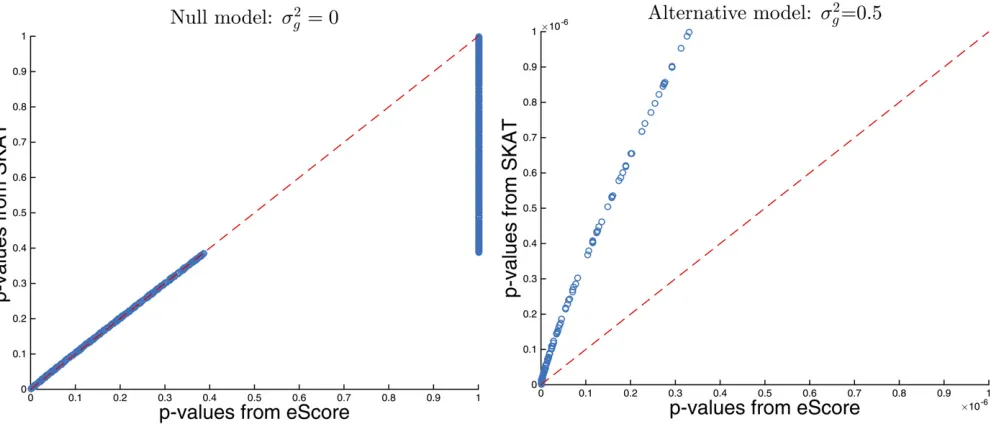
Figure 1 Discrepancy between SKAT and eScore P-values. Left: there is no SNP set effectðnull model; s2

g¼0Þ: Right: there is SNP set effect

ðalternative model; s2

g¼0:5Þ:

(3)

genome-wide studies. Detailed derivations are delegated to the Supplemental Material,File S1.

eScore

The classical score test statistic for testingH0:s2g¼0 (no SNP

set effect)vs. HA:s2g.0 takes the form

Sscore¼

J21 s2

g;s2g

_@

@s2 gL

2 @

@s2

g

L.0

0 @

@s2

g

L#0 ; 8 > > > < > > > :

whereJis the Fisher information matrix relevant to variance components ðs2

g;s2eÞ and _@@_s2

gL is the score function, both

evaluated at the maximum likelihood estimate (MLE) under H0:File S1, section S.2, shows that

Sscore¼max ðy2X ^

bÞ9Sðy2Xb^Þ ðy2Xb^Þ9ðy2Xb^Þ;

trðSÞ n

( )

; (3)

whereb^¼ ðX9XÞ21X9yis the least squares estimate ofﬁxed effects and trðMÞrepresents the sum of diagonal entries of a square matrixM:The exact score test (eScore) rejects the null hypothesis whenSscoreis large.

Lets¼rankðXÞ;PX¼XðX9XÞ21X9be the projection ma-trix onto the column space CðXÞ; and fm1;. . .;mkg be the

strictly positive eigenvalues of ðIn2PXÞSðIn2PXÞ: Under the null hypothesiss2

g¼0;Sscoreis distributed as max

Pk i¼1mkw2i

Pn2s i¼1w2i

;trðSÞ

n

( )

;

wherew1;. . .;wn2sare independent standard normals. The

P-value of observedSScore¼tequals the tail probability

P

Pk i¼1mix21;i

Pn2s i¼1x21;i

$t

!

¼P X k

i¼1

ðmi2tÞx21;i2tx2n2s2k$0

!

;

wherex2

1;1;. . .;x21;k;x

2

n2s2k are independent chi-square

ran-dom variables. Therefore eScoreP-values can be calculated

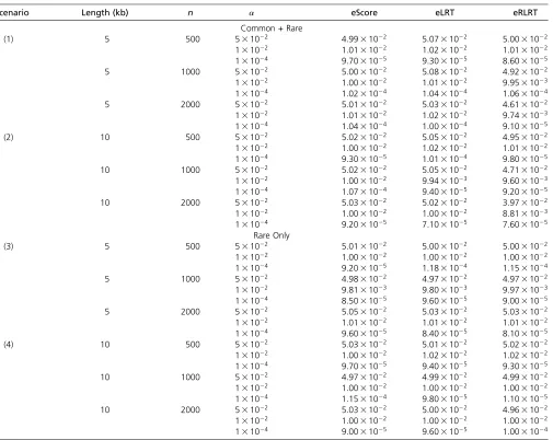
Table 1 Empirical type I error rate of eScore, eLRT, and eRLRT based on 106_{simulation replicates}

Scenario Length (kb) n a eScore eLRT eRLRT

Common + Rare

(1) 5 500 531022 ₄_:₉₉₃₁₀22 ₅_:₀₇₃₁₀22 ₅_:₀₀₃₁₀22

131022 ₁_:₀₁₃₁₀22 ₁_:₀₂₃₁₀22 ₁_:₀₁₃₁₀22 131024 ₉_:₇₀₃₁₀25 ₉_:₃₀₃₁₀25 ₈_:₆₀₃₁₀25 5 1000 531022 ₅_:₀₀₃₁₀22 ₅_:₀₈₃₁₀22 ₄_:₉₂₃₁₀22 131022 ₁_:₀₀₃₁₀22 ₁_:₀₁₃₁₀22 ₉_:₉₅₃₁₀23 131024 ₁_:₀₂₃₁₀24 ₁_:₀₄₃₁₀24 ₁_:₀₆₃₁₀24 5 2000 531022 ₅_:₀₁₃₁₀22 ₅_:₀₃₃₁₀22 ₄_:₆₁₃₁₀22 131022 ₁_:₀₁₃₁₀22 ₁_:₀₂₃₁₀22 ₉_:₇₄₃₁₀23 131024 ₁_:₀₄₃₁₀24 ₁_:₀₀₃₁₀24 ₉_:₁₀₃₁₀25

(2) 10 500 531022 ₅_:₀₂₃₁₀22 ₅_:₀₅₃₁₀22 ₄_:₉₅₃₁₀22

131022 ₁_:₀₀₃₁₀22 ₁_:₀₂₃₁₀22 ₁_:₀₁₃₁₀22 131024 ₉_:₃₀₃₁₀25 ₁_:₀₁₃₁₀24 ₉_:₈₀₃₁₀25 10 1000 531022 ₅_:₀₂₃₁₀22 ₅_:₀₅₃₁₀22 ₄_:₇₁₃₁₀22 131022 ₁_:₀₀₃₁₀22 ₉_:₉₄₃₁₀23 ₉_:₆₀₃₁₀23 131024 ₁_:₀₇₃₁₀24 ₉_:₄₀₃₁₀25 ₉_:₂₀₃₁₀25 10 2000 531022 ₅_:₀₃₃₁₀22 ₅_:₀₂₃₁₀22 ₃_:₉₇₃₁₀22 131022 ₁_:₀₀₃₁₀22 ₁_:₀₀₃₁₀22 ₈_:₈₁₃₁₀23 131024 ₉_:₂₀₃₁₀25 ₇_:₁₀₃₁₀25 ₇_:₆₀₃₁₀25

Rare Only

(3) 5 500 531022 ₅_:₀₁₃₁₀22 ₅_:₀₀₃₁₀22 ₅_:₀₀₃₁₀22

131022 ₁_:₀₀₃₁₀22 ₁_:₀₀₃₁₀22 ₁_:₀₀₃₁₀22 131024 ₉_:₂₀₃₁₀25 ₁_:₁₈₃₁₀24 ₁_:₁₅₃₁₀24 5 1000 531022 ₄_:₉₈₃₁₀22 ₄_:₉₇₃₁₀22 ₄_:₉₇₃₁₀22 131022 ₉_:₈₁₃₁₀23 ₉_:₈₀₃₁₀23 ₉_:₉₇₃₁₀23 131024 ₈_:₅₀₃₁₀25 ₉_:₆₀₃₁₀25 ₉_:₀₀₃₁₀25 5 2000 531022 ₅_:₀₅₃₁₀22 ₅_:₀₃₃₁₀22 ₅_:₀₃₃₁₀22 131022 ₁_:₀₁₃₁₀22 ₁_:₀₁₃₁₀22 ₁_:₀₁₃₁₀22 131024 ₉_:₆₀₃₁₀25 ₈_:₄₀₃₁₀25 ₈_:₁₀₃₁₀25

(4) 10 500 531022 ₅_:₀₃₃₁₀22 ₅_:₀₁₃₁₀22 ₅_:₀₂₃₁₀22

131022 ₁_:₀₀₃₁₀22 ₁_:₀₂₃₁₀22 ₁_:₀₂₃₁₀22 131024 ₉_:₇₀₃₁₀25 ₉_:₄₀₃₁₀25 ₉_:₃₀₃₁₀25 10 1000 531022 ₄_:₉₇₃₁₀22 ₄_:₉₉₃₁₀22 ₄_:₉₉₃₁₀22 131022 ₁_:₀₀₃₁₀22 ₁_:₀₀₃₁₀22 ₁_:₀₀₃₁₀22 131024 ₁_:₁₅₃₁₀24 ₉_:₈₀₃₁₀25 ₁_:₁₀₃₁₀25 10 2000 531022 ₅_:₀₃₃₁₀22 ₅_:₀₀₃₁₀22 ₄_:₉₆₃₁₀22 131022 ₁_:₀₀₃₁₀22 ₁_:₀₀₃₁₀22 ₁_:₀₀₃₁₀22 131024 ₉_:₀₀₃₁₀25 ₉_:₆₀₃₁₀25 ₁_:₀₀₃₁₀24

(4)

using the same numerical methods SKAT uses to evaluate the tail probability of a mixture of independent chi-squares. Moreover, whenever the ratio of two quadratic forms in (3) is less than the threshold n21_tr_ð_S_Þ_; _{it represents evidence} against the alternative hypothesis and the correct P-value should be 1. This saves considerable computation as most test regions are not associated with the trait.

In contrast, SKAT employs the test statistic

SSKAT¼

ðy2Xb^Þ9Sðy2XbÞ ðy2Xb^Þ9ðy2Xb^Þ=ðn2sÞ¼

ðy2Xb^Þ9Sðy2Xb^Þ ^

s2

e

(4)

and calculates its P-value using the null distribution

Pk

i¼1mix21;iofs2e2ðy2Xb^Þ9Sðy2Xb^Þ:Under the null model,

^ s2

e converges to the true s2e as sample size n increases.

ThereforeSSKATis distributed as

Pk

i¼1mix21;ionly

asymptot-ically. Under the alternative modelðs2

g6¼0Þ;however,s^

2

eis

a biased estimator that tends to overestimate the trues2

e:

This bias potentially affects the power ofSSKAT:

eLRT and eRLRT

In this section weﬁrst review the eLRT and eRLRT for testing a single variance component proposed by Crainiceanu and Ruppert (2004), and then discuss the computational chal-lenges for applying them to sequencing studies. Section S.3 inFile S1gives self-contained derivation.

The LRT statistic for testingH0:s2g¼0vs. HA:s2g.0 is

SLRT¼2 sup

HA

Lb;s2_g;s2_e22 sup H0

Lb;s2_g;s2_e: (5)

Under the null models2

g¼0;SLRT has exact distribution

SLRT¼D sup l$0

nln

Xn2s i¼1w

2

i

Xk i¼1

w2

i 1þlmi

þXn2s

i¼kþ1w 2 i 8 > > > < > > > :

2Xl

i¼1

lnð1þljiÞ

)

; (6)

where w1;. . .;wn2s are independent standard normals,

j1;. . .;jℓ are the strictly positive eigenvalues of S; and

fm1;. . .;mkg are the strictly positive eigenvalues of

ðIn2PXÞSðIn2PXÞ:

The RLRT is based on the restricted/residual log-likelihood

RLs2g;s2e

¼ 2n2s

2 lnð2pÞ2 1 2lndet

Q9VQ

21

2y9Q

Q9VQ21Q9y;

(7)

whereI2PX¼QQ9:The RLRT statistic is

SRLRT¼2 sup

HA

RLs2_g;s2_e22 sup H0

RLs2_g;s2_e; (8)

which, under the null models2

g¼0;has exact distribution

SRLRT¼D sup l$0

ðn2sÞln

Xn2s i¼1w

2

i

Xk i¼1

w2_i 1þlmi

þXn2s

i¼kþ1w 2 i 8 > > > < > > > : 2X k

i¼1

lnð1þlmiÞ

)

; (9)

where w1;...;wn2s are independent standard normals and

fm1;. . .;mkg are the strictly positive eigenvalues of

ðIn2PXÞSðIn2PXÞ:

Applying eLRT and eRLRT to NGS studies, which routinely test 103106 genes or SNP sets, incurs serious computa-tional challenges. First we need toﬁnd the MLEðb^;s^2

g;s^

2

eÞ

or restricted maximum likelihood estimate (REML)ðs^2g;s^

2

eÞ

for each SNP set, which requires repeatedly invertingn3n matrices, an expensive operation when n is large. Second, computing the P-value of eLRT or eRLRT for each SNP set is nontrivial. Crainiceanu and Ruppert (2004) propose the straightforward way of simulating B points from the null distribution (6) or (9). That involves solving B univariate optimizations, whereBneeds to be at order of 106_{to obtain} P-values at order of 1024_{with accuracy. This method is hard} to scale to genomic scans with a large number of SNP sets.

Implementation

We attack thefirst computational challenges by an efficient and stable algorithm forfitting the alternative model that avoids repeatedly inverting matrices. We resolve the second challenge by using an accurate approximation that only requires simu-lating a small number of points from the null distributions.

Fast algorithm forﬁtting variance component model

This section describes an efﬁcient algorithm for ﬁtting the variance component Model 2 or restricted-likelihood Model 7. Let S¼Udiagðj1;. . .;jnÞU9be the eigen decomposition of

the SNP set variance matrix. Then

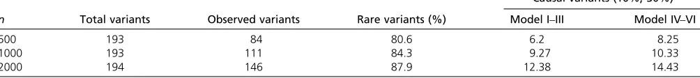
Table 2 Summary of testing regions (average over simulation replicates)

n Total variants Observed variants Rare variants (%)

Causal variants (10%, 30%)

Model I–III Model IV–VI

500 193 84 80.6 6.2 8.25

1000 193 111 84.3 9.27 10.33

2000 194 146 87.9 12.38 14.43

(5)

Lb;s2_e;s2_g¼ 2n

2lnð2pÞ2 1 2

Xn

i¼1

lns2_e þs2_gji

21

2ðy2X~bÞ9diagðwÞð~y2~XbÞ;

where y~¼U9y; X~¼U9X; and w¼ fðs2

eþs2gj1Þ2 1

;...;

ðs2

eþs2gjnÞ2

1_g

Our strategy is to update the mean compo-nents b and variance components ðs2

e;s2gÞ alternately.

Updating b given ðs2

e;s2gÞ is a standard weighted

least-squares problem. To update ðs2

e;s2gÞgivenbð

tÞ_;_{where the}

superscripttis iteration number, we denote the residuals by rðtÞ_¼_~_y₂_X~_bðtÞ_:_{The objective is then}

21

2

Xn

i¼1

lns2_e þs2_gji

21

2

Xn

i¼1

rð_itÞ2s2_e þs2_gji

21

;

which can be maximized by a minorization-maximization (MM) technique (Hunter and Lange 2000). The simple MM updates are

s2ðtþ1Þ

e ¼s2eðtÞ

ffiffiffiffiffiffiffiffiffiffiffiffiffiffiffiffiffiffiffiffiffiffiffiffiffiffiffiffiffiffiffiffiffiffiffiffiffiffiffiffiffiffiffiffiffiffiffiffiffiffiffiffiffiffiffiffiffiffiffi Xn

i¼1r

ðtÞ2

i

s2ðtÞ

e þjis2gðtÞ

₂2

Xn i¼1

s2ðtÞ

e þjis2gðtÞ

₂1 v u u u u t

s2ðtþ1Þ

g ¼s2gðtÞ

ffiffiffiffiffiffiffiffiffiffiffiffiffiffiffiffiffiffiffiffiffiffiffiffiffiffiffiffiffiffiffiffiffiffiffiffiffiffiffiffiffiffiffiffiffiffiffiffiffiffiffiffiffiffiffiffiffiffiffiffiffiffi Xn

i¼1jir

ðtÞ2

i

s2ðtÞ

e þjis

2ðtÞ

g

₂2

Xn i¼1ji

s2ðtÞ

e þjis2gðtÞ

₂1 v u u u u t : (10)

See section S.4 inFile S1for the derivation of the MM up-dates. This algorithm avoids repeatedly invertingn3n ma-trices as only one eigen decomposition is required. Each iteration only involves solving a weighted least squares prob-lem andOðnÞoperations for updating variance components. This algorithm is numerical stable as each update ofband

ðs2

g;s

2

eÞalways increases the log-likelihood value.

For eRLRT, we need toﬁnd the REML for each SNP set. Let B2ℝn3ðn2sÞ _{be an orthonormal basis of} _C_ð_X_Þt_; _e.g._, obtained from the singular value decomposition ofX:Then B9Yis multivariate normal with mean0n2sand covariance

B9VB¼s2

eB9Bþs2gB9SB¼s2eIn2sþs2gB9SB:

Let the eigen decomposition of the covariance matrixB9SBbe

B9V1B¼Gdiagðj1;. . .;jn2sÞG9:

Then the transformed data Y~¼G9B9Y has independent components

~

Y N0n2s;s2eIn2sþs2gdiagðj1;. . .;jn2sÞ

and the restricted log-likelihood function (7) becomes

2n2s

2 lnð2pÞ2 1 2

Xn2s

i¼1

lns2e þs2gji

21

2

X

n2s

i¼1 ~ y2i

s2

e þs2gji

21

:

It becomes clear that the MM updates (10) remain unchanged forﬁnding REML except replacingriby~yiandnbyn2s:

Approximating null distributions of eLRT and eRLRT

Calculation of eLRT and eRLRT P-values relies on drawing samples from the theoretical null distributions (6) and (9). Typical genome scans test 103₁₀5 _{SNP sets. An} exome-wide signiﬁcantP-value at a level of 1026 _{requires drawing} about 107 _{samples from the null distribution and each of} them requires solving a univariate optimization problem. Hence theP-value calculation for eLRT and eRLRT is compu-tationally intensive. We propose an approximation scheme that only requires drawing a small number of samples for each SNP set and thus is highly scalable to genomic scans.

We approximate the exact null distributions (6) and (9) by a mixture distribution of formp0x20:ð12p0Þax2b;where the

point mass p0 at 0, scale parameter a, and the degree of freedombfor the chi-squared distribution need to be deter-mined for each SNP set. We illustrate with eLRT. Denote the expression to be maximized in (6) byfðlÞ:The point mass of the null distribution at 0 is well approximated by the proba-bility offðlÞhaving a local maximum at 0

Probf9ðlÞ#0¼Prob

Xk i¼1miw

2

i

Xn2s i¼1w

2

i

#1 n

Xℓ

i¼1 ji ! ¼Prob 0 B B @ Xk

i¼1

0 B B

@mi2n21

Xℓ

i9¼1 ji9

1 C C A

x2

i 2 n21

Xℓ

i9¼1 ji9

!

x2

n2s2k#0

1 C C A:

Thereforep0 is calculated by either numerically evaluating the cumulative distribution function of the mixture of chi-square distribution at 0 or by the simple Monte Carlo method. To approximate the continuous partax2

bof null distribution,

we simulate a small number (300 by default) of SLRT by numerically maximizing fðlÞusing the Newton–Raphson method, and then estimate parametersaandbby matching theﬁrst two sample moments to those ofax2

b:This

approxi-mation scheme is well known as the Satterthwaite method in statistics (Satterthwaite 1941), which has been used

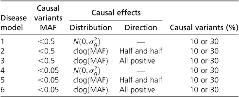
Table 3 Models for simulating phenotypes based on a 10-kb region

Disease model

Causal

variants Causal effects

Causal variants (%)

MAF Distribution Direction

1 ,0.5 Nð0;s2

gÞ — 10 or 30

2 ,0.5 clogðMAFÞ Half and half 10 or 30 3 ,0.5 clogðMAFÞ All positive 10 or 30 4 ,0.05 Nð0;s2

gÞ — 10 or 30

(6)

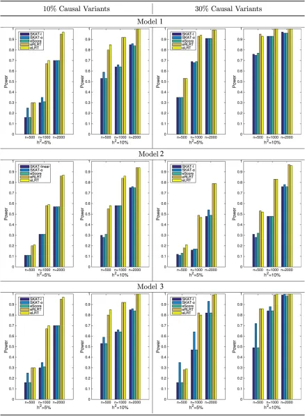
Figure 2 Power comparison when causal variants are both common and rare (Models 1–3). Left panel shows the power when 10% of the variants in the testing region are causal; right panel shows the power when 30% of the variants in the testing region are causal. Heritability is ﬁxed at both 5 and 10%.

(7)

(8)

successfully to approximate the null distributions of many test statistics. The performance of our approximation is in-cluded in the section S.5 inFile S1, which indicates that our approximation method works well for generating P-values and reducing computational burden.

Data availability

Simulated data sets are generated using computing language JULIAand are available upon request. COPDGene exome

se-quencing study (http://www.copdgene.org/) is part of the National Heart, Lung, and Blood Institute (NHLBI) Grand Opportunity Exome Sequencing Project (GO-ESP) and has been deposited to database of Genotypes and Phenotypes (dbGaP) (study accession: phs000296.v3.p2).

Results

Weﬁrst illustrate the subtle differences between SKAT and eScore for the motivation of exact tests. We then conduct a comprehensive simulation study to illustrate the control of type I error rate and the power under various conditions of genetic association. These simulations were designed to eval-uate two primary questions: (1) What is the relative perfor-mance and what are the advantages of using LRT based tests, especially when the causal variants are rare? (2) Can our method still have advantages even when genetic association are not under model assumptions?

Simulation studies

Differences between SKAT and eScore are demonstrated using simulations. Genotypes of n¼200 samples are formed by randomly pairing 400 haplotypes drawn from the haplotype pool distributed with the SKAT software (Wuet al.2011). We used theﬁrst 5 kb as the test region, which contains 61 monomorphic loci, 20 rare variants with MAF (minor allele frequency) ,0.05 (13 with MAFs

,0:01), and 12 common SNPs. 1000 replicates ofy are generated under the null ðs2

g¼0Þ and alternative model

ðs2

g¼0:5Þ; respectively. Under the alternative

hypothe-ses, causal variants are chosen using criterion MAF

,0:05:For simplicity no covariates are included. Figure 1 displays the discrepancy ofP-values between eScore and SKAT. Under the null model (left panel), SKAT P-values roughly match those from eScore, except 73.1% of the eScore tests haveP-values equal to 1. This reﬂects the fact that s^2e is a fairly accurate estimate ofs2e under the null

model. Under the alternative model (right panel), how-ever, s^2e is a biased estimate and the SKAT P-values are

systematically larger than those from eScore, especially in the region of small P-values. This can lead to loss of power by SKAT in genome scans where a stringentP-value threshold is necessary to correct multiple testing. The dif-ference is more dramatic at smaller sample sizes or stron-ger effect sizes2

g:

For both type I error and power simulation studies, we use the haplotype pool that comes with the SKAT software

(Wuet al.2011) to generate genotypes of study samples. That is, for each simulation replicate, we pair 2n ran-domly drawn haplotypes to form the genotypes of a sample of n subjects. To assess empirical type I error of eScore, eLRT, and eRLRT, we consider combinations of following factors:

1. test region:ﬁrst 5 or 10 kb,

2. samples sizen: 500, 1000, or 2000, and 3. signiﬁcance levela: 0.05, 0.01, or 0.0001.

The average number of variants are 97 and 193 for 5- and 10-kb regions, respectively. We evaluate type I error when both common and rare variants are included in the region as well as when only rare variants (MAF,5%) are included in the region. We generate 106 _{replicates for each simulation} scenario. For each replicate, weﬁrst simulate four continuous covariates from independent standard normals, one binary covariate from Bernoulli(0.5), and then generate phenotypes from Model 1 with b¼1; s2

g¼0; and s2e ¼1: Results in

Table 1 show that the three exact tests control type I error at allalevels.

For power comparisons, we take the ﬁrst 10 kb of the haplotype pool as the test region. Over simulation replicates, testing regions include around 193 variants and 80–150 ob-served variants on average (Table 2). Average proportion of rare variants (MAF ,0.05) are 80.8, 84.3, and 87.9% for sample sizes of 500, 1000, and 2000, respectively. The num-ber of causal variants for different models are also shown in Table 2. This is among the settings where we have evaluated protected type I error. Covariates are generated in the same manner as in the last section and we setﬁxed effects atb¼1: For Models 1 and 4, causal effectsgfollow a normal distri-butionNð0;s2

gIÞ:Models 2, 3, 5, and 6 mimic the simulation

schemes in Wuet al.(2010), where the magnitude of causal effectsgis determined bycjlogðMAFÞj;so that rarer variants have larger effects. In Wuet al.’s (2010) article,cwas set up as 0.4 and in Leeet al.’s (2014) articlecwas set as 0.14, which provides 80% power at levela,1028_{when the sample size} is 50,000. In our simulations, we chose s2

g and c by ﬁxing

heritabilityh2_;_where_h2_¼_Var_ð_G_g_Þ₌_Var_ð_Y_Þ_;_{so that power is} in the comparable ranges for most of methods given sample sizes. Environmental variances2

e wasﬁxed at 1. For Models

1 and 4, we choses2

gto be,

s2

g¼

h2 12h2:

Table 4 The number of gene sets that pass genome-wide signiﬁcant level at FWER 0.05 from the COPDGene exome sequencing study

eScore eRLRT eLRT SKAT SKAT-o

Height 5 8 15 4 3

PackYears 0 0 0 0 0

BMI 0 0 0 0 0

For eScore, eRLRT, eLRT, and SKAT, linear kernel and no weights are adopted.

(9)

Similarly,cwas chosen according to the formula

c¼

ffiffiffiffiffiffiffiffiffiffiffiffiffiffiffiffiffiffiffiffiffiffiffiffiffiffiffiffiffiffiffiffiffiffiffiffiffiffiffiffiffiffiffiffiffiffiffiffiffiffiffiffi

h2

12h2

1

VarðGjlogðMAFÞjÞ

s

:

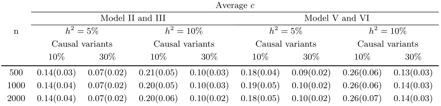
As a comparison we list the mean and standard deviation of our simulatedcover simulation replicated inFile S1(Table S1). It is shown that ourcis smaller compared to Wuet al.(2010) and Leeet al.(2014), which indicates smaller heritability explained by testing regions. We consider the following simulation factors to evaluate power and label them as Models 1–6 in Table 3:

1. sample sizen: 500, 1000, or 2000, 2. heritabilityh2_:_{5 or 10%,}

3. MAF of causal variants: common and rare (MAF,0.5) or rare only (MAF,0.05),

4. percentage of causal variants: 10 or 30%, 5. distribution of causal effects:Nð0;s2

gÞorcjlogðMAFÞj;

6. direction of causal effects: half positive and half negative or all positive.

Significant level a is 1024_: _{We simulate 1000} repli-cates for each scenario. Therefore the largest Monte Carlo standard error for power estimate is controlled below_{ffiffiffiffiffiffiffiffiffiffiffiffiffiffiffiffiffiffiffiffiffiffiffiffiffiffiffiffiffiffiffiffiffiffiffiffiffiffiffiffiffiffiffiffi}

0:53ð120:5Þ=1000

p

0:016:

For simplicity, in both simulation and real data analysis, SNP weights are not incorporated and the linear kernel is adopted for both exact tests and SKAT. SKAT optimal (SKAT-o)

uses the default setting in Lee et al. (2012). Note all exact tests can incorporate variant weights or other kernels just as in SKAT or SKAT-o.

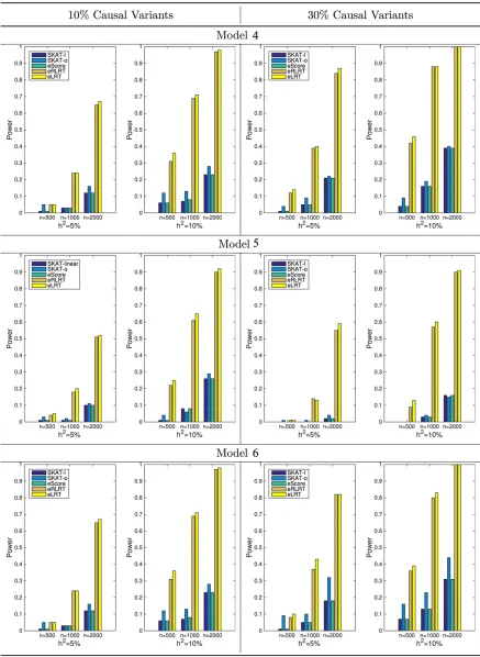
Figure 2 displays the results for Models 1, 2, and 3 (common and rare causal variants) and Figure 3 for Models 4, 5, and 6 (rare causal variants only). Left panels of both ﬁgures are the results when 10% of the variants in the region are causal, while the right panels show powers when 30% of variants are causal. It is clear that (1) performance of score tests (SKAT and eScore) are comparable in these scenarios; (2) eLRT and eRLRT signiﬁcantly boosts power over score tests across all scenarios, especially when causal variants are rare only or sample size is small; and (3) when the causal variants are both common and rare, the SKAT-o method can increase power extensively pared with SKAT method with linear kernel. Its power is com-parable to eLRT and eRLRT (Figure 2).

COPDGene exome sequencing study

We further illustrate our methods using the COPDGene exome sequencing study (http://www.copdgene.org/). It is part of

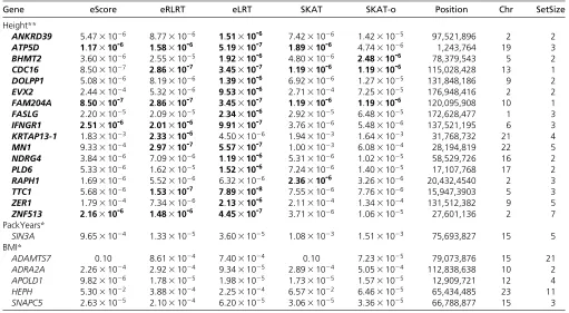
Table 5 Top genes from the COPDGene exome sequencing study usingﬁve different methods

Gene eScore eRLRT eLRT SKAT SKAT-o Position Chr SetSize

Height**

ANKRD39 5:4731026 ₈_:₇₇₃₁₀26 ₁_:₅₁₃_10-6

7:4231026 ₁_:₄₂₃₁₀25 _97,521,896 ₂ ₂ ATP5D 1:17310-6 1:58310-6 5:19310-7 1:89310-6 4:7431026 _1,243,764 ₁₉ ₃ BHMT2 3:6031026 ₂_:₅₅₃₁₀25 ₁_:₉₂₃_10-6

4:8031026 ₂_:₄₈₃_10-6

78,379,543 5 2

CDC16 8:5031027 ₂_:₈₆₃_10-7

3:45310-7 1:19310-6 1:19310-6 115,028,428 13 1 DOLPP1 5:0831026 ₈_:₁₉₃₁₀26 ₁_:₃₉₃_10-6

6:9231026 ₁_:₂₇₃₁₀25 _131,848,186 ₉ ₂ EVX2 2:4431024 ₅_:₃₂₃₁₀26 ₉_:₅₃₃_10-6

2:7131024 ₇_:₂₅₃₁₀25 _176,948,416 ₂ ₂ FAM204A 8:50310-7 ₂_:₈₆₃_10-7 ₃_:₄₅₃_10-7 ₁_:₁₉₃_10-6 ₁_:₁₉₃_10-6 _120,095,908 ₁₀ ₁ FASLG 2:2031025 ₂_:₀₉₃₁₀25 ₂_:₃₄₃_10-6 ₂_:₉₂₃₁₀25 ₆_:₄₈₃₁₀25 _172,628,477 ₁ ₃ IFNGR1 2:51310-6 ₂_:₀₁₃_10-6 ₉_:₉₁₃_10-7 ₃_:₇₆₃₁₀26 ₅_:₄₈₃₁₀26 _137,521,195 ₆ ₃ KRTAP13-1 1:8331023 ₂_:₃₃₃_10-6 ₄_:₅₀₃₁₀26 ₁_:₉₄₃₁₀23 ₁_:₆₄₃₁₀23 _31,768,732 ₂₁ ₄ MN1 9:3331024 ₂_:₉₇₃_10-7 ₅_:₅₇₃_10-7 ₁_:₀₀₃₁₀23 ₆_:₀₈₃₁₀24 _28,194,819 ₂₂ ₅ NDRG4 3:8431026 ₇_:₀₉₃₁₀26 ₁_:₁₉₃_10-6 ₅_:₃₁₃₁₀26 ₁_:₀₂₃₁₀25 _58,529,726 ₁₆ ₂ PLD6 5:3331026 ₁_:₆₂₃₁₀25 ₁_:₅₂₃_10-6 ₇_:₂₄₃₁₀26 ₁_:₄₀₃₁₀25 _17,107,768 ₁₇ ₂ RAPH1 1:6931026 ₅_:₅₂₃₁₀26 ₆_:₃₂₃₁₀26 ₂_:₃₆₃_10-6 ₃_:₂₆₃₁₀26 _20,432,4540 ₂ ₃ TTC1 5:6831026 ₁_:₅₃₃_10-7 ₇_:₈₉₃_10-8 ₇_:₅₅₃₁₀26 ₇_:₇₆₃₁₀26 _15,947,3903 ₅ ₃ ZER1 1:7931024 ₇_:₃₄₃₁₀26 ₂_:₁₃₃_10-6 ₂_:₁₁₃₁₀24 ₁_:₃₄₃₁₀24 _131,512,382 ₉ ₅ ZNF513 2:16310-6 1:48310-6 4:45310-7 3:7131026 ₁_:₀₆₃₁₀25 _27,601,136 ₂ ₇ PackYears*

SIN3A 9:6531024 ₁_:₃₃₃₁₀25 ₃_:₆₀₃₁₀25 ₁_:₀₈₃₁₀23 ₁_:₅₁₃₁₀23 _75,693,827 ₁₅ ₅ BMI*

ADAMTS7 0.10 8:6131024 ₇_:₄₀₃₁₀24 _0.10 ₇_:₂₃₃₁₀25 _79,073,876 ₁₅ ₂₁ ADRA2A 2:2631024 ₂_:₉₂₃₁₀24 ₉_:₃₄₃₁₀25 ₂_:₈₉₃₁₀24 ₅_:₀₅₃₁₀24 _112,838,638 ₁₀ ₂ APOLD1 9:8231026 ₁_:₇₈₃₁₀25 ₁_:₉₈₃₁₀25 ₁_:₇₃₃₁₀25 ₁_:₅₇₃₁₀25 _12,909,721 ₁₂ ₄ HEPH 5:3031022 ₃_:₈₈₃₁₀24 ₂_:₂₅₃₁₀24 ₆_:₅₇₃₁₀22 ₆_:₄₆₃₁₀25 _65,434,485 ₂₃ ₁₁ SNAPC5 2:6331025 ₂_:₁₀₃₁₀24 ₆_:₂₀₃₁₀25 ₃_:₀₆₃₁₀25 ₃_:₃₆₃₁₀25 _66,788,877 ₁₅ ₃

Genes that pass Bonferroni corrected genome-wide signiﬁcance level of 331026_{are in boldface font. Position is the base pair position in the middle of the gene. Chr,}

chromosome of the test region; SetSize, the number of SNPs in the test region.**P,331026_,_*_P_,₁₀24_.

Table 6 Runtimes (in seconds) of different methods

Trait SKAT SKAT-o eScore eLRT eRLRT

eight 61.6 4004.1 53.5 64.8 31.9

PackYears 61.2 4041.3 50.3 56.9 28.4

(10)

NHLBI GO-ESP project (dbGaP study accession: phs000296. v3.p2). After quality control, 399 individuals remain for the analysis (Qiaoet al.2016). We analyze 16;619 genes along the genome and apply different testing methods to three phenotypes: height, cigarette packages per year (PackYears), and body mass index (BMI). Table S2inFile S1 tabulates their descriptive statistics.

For all three phenotypes, we adjust population substruc-ture using the top three eigenvectors generated by the Eigen-strat software (Price et al. 2006), age, and gender. For PackYears, we additionally adjust for current smoking status. Table 4 shows the numbers of gene sets that pass Bonferroni-adjusted exome-wide significance level 331026_: _{Table 5} contains detailed information of gene sets that pass exome-wide significance level for height. It also lists gene sets with P-value ,1024_{for trait PackYears and BMI for the purpose} of side-by-side comparison ofP-values, as none of the gene sets pass the exome-wide significant level.

We make following observations: (1) For the complex trait height, eLRT and eRLRT identify 8 and 15 genes that pass the Bonferroni-adjusted, genome-wide significant level and eScore identifies 5. In contrast, SKAT and SKAT-o only identify four and three respectively. (2) For the other two traits, no genes pass Bonferroni-adjusted genome-wide significance level in all tests. (3) eScoreP-values are universally smaller than SKAT. This agrees with the simulation results in Figure 1 that the asymptotic test by SKAT can lose power at small samples size and strong signals. (4) The optimal kernel in SKAT-o does not show advantage over SKAT with linear ker-nel and no weight in this analysis (Figure S1).

Computational efﬁciency of ExactVC

We compare the computational time of different methods. Table 6 records the run times of each method on a desktop with i7-3770 central processing unit of 3.40 GHz and 16 GB RAM. For each trait, exact tests (eScore and eRLRT) complete the analysis in ,1 min, while eLRT uses around a minute. SKAT takes slightly longer than eScore, while SKAT-o takes signiﬁcantly longer than all of the tests. Note that although LRT and RLRT is considered more computationally intensive compared to the score test, Table 6 shows that the speed of our eLRT test is comparable to eScore and SKAT tests, while eRLRT is even faster.

Discussion

In this report we study and implement computationally effi -cient exact variance component tests (eScore, eLRT, and eRLRT) for testing SNP sets in sequencing studies. Simulation study and real data analysis show that (1) all exact tests control type I error, (2) eScore yields smallerP-values than SKAT at small sample size and strong signal, and (3) eLRT and eRLRT significantly boost power over eScore, SKAT, and SKAT-o, especially when sample size is small or there are plenty of rare variants. By supplying a fast and easy-to-use software package, we hope to boost the power and efficiency

of gene mapping based on current NGS technology. Although the derivation of eLRT and eRLRT require normal assumption of genetic effects within a region, we evaluate the

misspeci-ﬁed distribution and how that will affect power. In all scenar-ios, even without normal assumption, our methods show superior power compared with competing methods. The soft-ware package, EXACTVCTEST, is implemented in the open source, high-performance technical computing language JULIAand is freely available athttps://github.com/Tao-Hu/

VarianceComponentTest.jl.

There are a few directions for future work. One advantage of the asymptotic test by SKAT is that it does not depend on the normality assumption and equally applies to association test-ing of binary traits (Wuet al.2011; Leeet al.2012), while the exact tests depend on the normality assumption. Fortunately many quantitative traits satisﬁes the normality assumption after suitable transformations. Development of LRT and RLRT for binary trait remains a challenge. Another statistical challenge is to develop LRT or RLRT for testing SNP set in related samples. An asymptotic score test has been developed by Chenet al.(2013). Rigorous testing of multiple variance components still remains a statistical challenge (Crainiceanu 2008; Drikvandiet al.2013).

Acknowledgments

COPDGene study is supported by National Institutes of Health R01 HL-089856 and R01 HL-089897. The whole exome sequencing was supported by the National Heart, Lung, and Blood Institute Exome Sequencing Project. J.J.Z. is supported by National Institutes of Health grant K01 DK-106116, M.H.C. is supported by National Institutes of Health grant R01 HL-113264. H.Z. is partially supported by National Institutes of Health grants HG-006139, GM-105785, GM-53275, and National Science Foundation grant DMS-1055210. Full list of chronic obstructive pulmonary disease investigators unit core and clinical centers are included in theFile S1.

Literature Cited

Chen, D., and U. Gyllensten, 2015 Lessons and implications from

association studies and post-gwas analyses of cervical cancer. Trends Genet. 31: 41–54.

Chen, H., J. B. Meigs, and J. Dupuis, 2013 Sequence kernel

asso-ciation test for quantitative traits in family samples. Genet. Epi-demiol. 37: 196–204.

Chen, Z., and D. B. Dunson, 2003 Random effects selection in

linear mixed models. Biometrics 59: 762–769.

Crainiceanu, C. M., 2008 Likelihood ratio testing for zero variance components in linear mixed models, pp. 3–17 inRandom Effect and Latent Variable Model Selection, Vol. 192, edited by D. B. Dunson. Springer, New York.

Crainiceanu, C. M., and D. Ruppert, 2004 Likelihood ratio tests in linear mixed models with one variance component. J. R. Stat. Soc. Series B Stat. Methodol. 66: 165–185.

Drikvandi, R., G. Verbeke, A. Khodadadi, and V. P. Nia, 2013 Testing multiple variance components in linear mixed-effects models. Biostatistics 14: 144_–159.

(11)

Greven, S., C. M. Crainiceanu, H. Küchenhoff, and A. Peters, 2008 Restricted likelihood ratio testing for zero variance com-ponents in linear mixed models. J. Comput. Graph. Stat. 17: 870–891.

Hunter, D. R., and K. Lange, 2000 Quantile regression via an MM

algorithm. J. Comput. Graph. Stat. 9: 60–77.

Kinney, S. K., and D. B. Dunson, 2007 Fixed and random effects

selection in linear and logistic models. Biometrics 63: 690–698. Lee, S., M. J. Emond, M. J. Bamshad, K. C. Barnes, M. J. Riederet al., 2012 Optimal uniﬁed approach for rare-variant association test-ing with application to small-sample case-control whole-exome sequencing studies. Am. J. Hum. Genet. 91: 224_–237.

Lee, S., G. R. Abecasis, M. Boehnke, and X. Lin, 2014 Rare-variant association analysis: study designs and statistical tests. Am. J. Hum. Genet. 95: 5–23.

Li, B., and S. M. Leal, 2008 Methods for detecting associations

with rare variants for common diseases: application to analysis of sequence data. Am. J. Hum. Genet. 83: 311–321.

Madsen, B. E., and S. R. Browning, 2009 A groupwise association

test for rare mutations using a weighted sum statistic. PLoS Genet. 5: e1000384.

Morgenthaler, S., and W. G. Thilly, 2007 A strategy to discover

genes that carry multi-allelic or mono-allelic risk for common diseases: a cohort allelic sums test (cast). Mutat. Res. Fundam.

Mol. Mech. Mutagen. 615: 28–56.

Price, A. L., N. J. Patterson, R. M. Plenge, M. E. Weinblatt, N. A. Shadicket al., 2006 Principal components analysis corrects for stratiﬁcation in genome-wide association studies. Nat. Genet. 38: 904–909.

Price, A. L., G. V. Kryukov, P. I. de Bakker, S. M. Purcell, J. Staples et al., 2010 Pooled association tests for rare variants in exon-resequencing studies. Am. J. Hum. Genet. 86: 832_–838. Psychiatric GWAS Consortium Bipolar Disorder Working Group,

2011 Large-scale genome-wide association analysis of bipolar

disorder identiﬁes a new susceptibility locus near ODZ4. Nat. Genet. 43: 977–983.

Qiao, D., C. Lange, T. H. Beaty, J. D. Crapo, K. C. Barnes et al.,

2016 Exome sequencing analysis in severe, early-onset chronic

obstructive pulmonary disease. Am. J. Respir. Crit. Care Med. 193: 1353–1363.

Qu, L., T. Guennel, and S. L. Marshall, 2013 Linear score tests for variance components in linear mixed models and applications to genetic association studies. Biometrics 69: 883–892.

Satterthwaite, F. E., 1941 Synthesis of variance. Psychometrika 6: 309–316.

Saville, B. R., and A. H. Herring, 2009 Testing random effects in the linear mixed model using approximate bayes factors. Bio-metrics 65: 369–376.

Wang, K., M. Li, and M. Bucan, 2007 Pathway-based approaches

for analysis of genomewide association studies. Am. J. Hum. Genet. 81: 1278_–1283.

Wang, K., M. Li, and H. Hakonarson, 2010 Analysing biological

pathways in genome-wide association studies. Nat. Rev. Genet. 11: 843–854.

Wang, K., H. Zhang, S. Kugathasan, V. Annese, J. P. Bradﬁeldet al.,

2009 Diverse genome-wide association studies associate the

il12/il23 pathway with crohn disease. Am. J. Hum. Genet. 84: 399–405.

Wu, M. C., P. Kraft, M. P. Epstein, D. M. Taylor, S. J. Chanocket al.,

2010 Powerful SNP-set analysis for case-control genome-wide

association studies. Am. J. Hum. Genet. 86: 929–942.

Wu, M. C., S. Lee, T. Cai, Y. Li, M. Boehnke et al., 2011

Rare-variant association testing for sequencing data with the se-quence kernel association test. Am. J. Hum. Genet. 1: 82–93. Zeng, P., and T. Wang, 2015 Bootstrap restricted likelihood ratio

test for the detection of rare variants. Curr. Genomics 16: 194– 202.

Zeng, P., Y. Zhao, J. Liu, L. Liu, L. Zhanget al., 2014 Likelihood ratio tests in rare variant detection for continuous phenotypes.

Ann. Hum. Genet. 78: 320_–332.

Zeng, P., Y. Zhao, H. Li, T. Wang, and F. Chen, 2015 Permutation-based variance component test in generalized linear mixed model with application to multilocus genetic association study. BMC Med. Res. Methodol. 15: 37.

(12)

eLRT

eRLRT

n=500

Monte Carlo

0 0.1 0.2 0.3 0.4 0.5 0.6 0.7 0.8 0.9 1

χ

2 Approximation

0 0.1 0.2 0.3 0.4 0.5 0.6 0.7 0.8 0.9 1 Monte Carlo

0 0.02 0.04 0.06 0.08 0.1 0.12 0.14 0.16 0.18 0.2

χ

2 Approximation

0 0.02 0.04 0.06 0.08 0.1 0.12 0.14 0.16 0.18 0.2 Monte Carlo

0 0.1 0.2 0.3 0.4 0.5 0.6 0.7 0.8 0.9 1

χ

2 Approximation

0 0.1 0.2 0.3 0.4 0.5 0.6 0.7 0.8 0.9 1 Monte Carlo 0 0.05 0.1 0.15 0.2 0.25 0.3 0.35

χ

2 Approximation

0 0.05 0.1 0.15 0.2 0.25 0.3 0.35

n=1000

Monte Carlo

0 0.1 0.2 0.3 0.4 0.5 0.6 0.7 0.8 0.9 1

χ

2 Approximation

0 0.1 0.2 0.3 0.4 0.5 0.6 0.7 0.8 0.9 1 Monte Carlo

0 0.05 0.1 0.15 0.2 0.25

χ

2 Approximation

0 0.05 0.1 0.15 0.2 0.25 Monte Carlo

0 0.1 0.2 0.3 0.4 0.5 0.6 0.7 0.8 0.9 1

χ

2 Approximation

0 0.1 0.2 0.3 0.4 0.5 0.6 0.7 0.8 0.9 1 Monte Carlo 0 0.05 0.1 0.15 0.2 0.25 0.3 0.35

χ

2 Approximation

0 0.05 0.1 0.15 0.2 0.25 0.3 0.35

n=2000

Monte Carlo

0 0.1 0.2 0.3 0.4 0.5 0.6 0.7 0.8 0.9 1

χ

2 Approximation

0 0.1 0.2 0.3 0.4 0.5 0.6 0.7 0.8 0.9 1 Monte Carlo 0 0.05 0.1 0.15 0.2 0.25

χ

2 Approximation

0 0.05 0.1 0.15 0.2 0.25 Monte Carlo

0 0.1 0.2 0.3 0.4 0.5 0.6 0.7 0.8 0.9 1

χ

2 Approximation

0 0.1 0.2 0.3 0.4 0.5 0.6 0.7 0.8 0.9 1 Monte Carlo 0 0.05 0.1 0.15 0.2 0.25 0.3 0.35

χ

2 Approximation

0 0.05 0.1 0.15 0.2 0.25 0.3 0.35

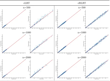
Figure S1:

Pvalues comparisons with and without 2 _{approximation for sample size 500, 1000, and 2000. Pvalues}

from eLRT tests are shown in columns one and two, while pvalues from eRLRT are shown in columns three and four. Second and forth columns are the zoom-in plots when pvalues are less than one. 1000 simulation replicates are included. Phenotypes are simulated under the null hypothesis and 10kb testing region is used for evaluation (e.g., scenario (2) in Table 3 of the manuscript). Red line represents the line with slope 1 and intercept 0.

(13)

n

Averagec

Model II and III Model V and VI

h2_{= 5%} _h2_{= 10%} _h2_{= 5%} _h2_{= 10%}

Causal variants Causal variants Causal variants Causal variants

10% 30% 10% 30% 10% 30% 10% 30%

500 0.14(0.03) 0.07(0.02) 0.21(0.05) 0.10(0.03) 0.18(0.04) 0.09(0.02) 0.26(0.06) 0.13(0.03) 1000 0.14(0.04) 0.07(0.02) 0.20(0.05) 0.10(0.03) 0.19(0.05) 0.10(0.02) 0.26(0.06) 0.14(0.03) 2000 0.14(0.04) 0.07(0.02) 0.20(0.06) 0.10(0.02) 0.18(0.05) 0.10(0.02) 0.26(0.07) 0.14(0.03)

(14)

Trait

Mean

SD

n

Height

(cm)

168.59

9.59

399 PackYears

50.05

19.73

399 BMI

26.92

5.04

399 Table S2: Descriptive statistics of 3 phenotypes in COPDGene exome sequencing study.

(15)

Supplemental Materials for

“ExactVC: Efficient Exact Variance Component Tests of SNP Sets”

Jin J. Zhou

1

_{, Tao Hu}

2,3

_{, Dandi Qiao}

4

_{, Michael H. Cho}

5,6,7

_{, Hua Zhou}

8

1

_{Division of Epidemiology and Biostatistics}

Mel and Enid Zuckerman College of Public Health

University of Arizona

Tucson, AZ 85724

2

_{Bioinformatics Research Center}

North Carolina State University

Raleigh, NC 27695

3

_{Department of Statistics}

North Carolina State University

Raleigh, NC 27695

4

_{Department of Biostatistics}

Harvard School of Public Health

5

_{Channing Division of Network Medicine}

Department of Medicine

Brigham and Women’s Hospital

6

_{Harvard Medical School}

7

_{Division of Pulmonary and Critical Care Medicine}

Department of Medicine

Brigham and Women?s Hospital

Boston, MA 02115

8

_{Department of Biostatistics}

University of California, Los Angeles

(16)

Corresponding author:

Jin Zhou

Division of Epidemiology and Biostatistics

Mel and Enid Zuckerman College of Public Health

University of Arizona, Tucson, AZ 85724

Phone: (520) 626-1393

Email: [email protected]

(17)

S.1 Model and notations

Suppose

y

is a

n

×

1 vector of quantitative phenotype,

X

is an

n

×

p

covariate matrix (e.g., grand

mean, sex, smoking history, height, principal components, etc),

β

is a

p

×

1 vector of fixed effects,

G

is an

n

×

m

genotype matrix for

m

genetic variants,

γ

is their effects and follows an normal

distribution with variance

σ

_g2

W

.

W

is the prespecified diagonal weight matrix for the rare variants

of size

m

×

m

.

ε

is the usual normal distributed random errors with mean zero and covariance

σ

_e2

I

n

. We consider a standard linear mixed model

y

=

Xβ

+

Gγ

+

ε

,

γ

∼

N

(

0

m

, σ

g2

W

), and

ε

∼

N

(

0

n

, σ

e2

I

n

) where

σ

2g

and

σ

2e

are corresponding variance component parameters for the SNP

set and environmental effects. Therefore, Var(

y

) =

V

=

σ

2_g

S

+

σ

_e2

I

n

, where

S

=

GW G

0

is the

kernel matrix capturing effects from the SNP set.

Throughout the paper, we let

P

X

=

X

(

X

0

X

)

−1

X

0

be the projection matrix onto the column

space of

C

(

X

),

I

n

−

P

X

be the projection matrix onto the complimentary null space of

N

(

X

0

) =

C

(

X

)

⊥

. Let

{

ξ

1

, . . . , ξ

`

}

be the positive eigenvalues of

S

and

{

µ

1

, . . . , µ

k

}

be the positive eigenvalues

of (

I

−

P

X

)

S

(

I

−

P

X

). We denote

l

= rank(

S

),

k

= rank((

I

−

P

X

)

S

(

I

−

P

X

)) and

s

= rank(

X

)

and define

Q

0

∈

R

n×s

be an orthonormal basis of

C

(

X

),

Q

1

∈

R

n×k

be an orthonormal basis from

the eigendecomposition of matrix (

I

−

P

X

)

S

(

I

−

P

X

),

Q

2

∈

R

n×(n−s−k)

is an orthonormal basis

of

C

(

Q

0,

Q

1

)

⊥

=

C

(

X

,

Q

1

)

⊥

, and

Q

= (

Q

1

,

Q

2

)

∈

R

n×(n−s)

be an orthonormal basis of the space

C

(

X

)

⊥

.

S.2 Derivation of eScore test statistic and null distribution

We derive the exact score test for

H

0

:

σ

g2

= 0 vs

H

A

:

σ

g2

>

0 in the variance component model

Y

∼

N

n

(

Xb

,

V

), where

V

=

σ

_e2

I

n

+

σ

g2

S

.

The log-likelihood function is

L

(

b

, σ

_e2

, σ

_g2

) =

−

n

2 ln(2

π

)

−

1

2 ln det(

V

)

−

1

2 (

y

−

Xb

)

0

_V

−1

₍

_y

₋

_Xb

₎

_.

and its partial derivative with respect to

σ

₁2

is

∂

∂σ

2

1

L

(

b

, σ

2₀

, σ

₁2

)

=

−

1

2 tr(

V

−1

_S

_{) +}

1

2 (

y

−

Xb

)

0

V

−1

SV

−1

(

y

−

Xb

)

.

The information matrix relevant to variance components has entries

E

−

∂

2

∂σ

2 e

∂σ

e2

L

=

1

2 tr(

V

−2

₎

E

−

∂

2

∂σ

2 e

∂σ

g2

L

=

E

−

∂

2

∂σ

2 g

∂σ

2e

L

=

1

2 tr(

V

−2

_S

₎

E

−

∂

2

∂σ

2 g

∂σ

g2

L

=

1

2 tr(

V

(18)

Rao’s score statistic is based on

J

_σ−21

g,σg2

∂

∂σ

2 g

L

2