Towards a dispersive determination of the pion transition form
factor
Stefan Leupold1,⋆, Martin Hoferichter2, Bastian Kubis3, Franz Niecknig3, and Sebastian P. Schneider3
1Institutionen för fysik och astronomi, Uppsala Universitet, Box 516, 75120 Uppsala, Sweden 2Institute for Nuclear Theory, University of Washington, Seattle, WA 98195-1550, USA
3Helmholtz-Institut für Strahlen- und Kernphysik (Theorie) and Bethe Center for Theoretical Physics, Univer-sität Bonn, 53115 Bonn, Germany
Abstract.We start with a brief motivation why the pion transition form factor is interest-ing and, in particular, how it is related to the high-precision standard-model calculation of the gyromagnetic ratio of the muon. Then we report on the current status of our ongoing project to calculate the pion transition form factor using dispersion theory. Finally we present and discuss a wish list of experimental data that would help to improve the input for our calculations and/or to cross-check our results.
1 Motivation
This presentation is closely related to the talks by B. Kubis and M. Procura; see also their contributions to these proceedings. The first parts of this presentation are based on [1] to which we refer for further details.
The pion transition form factor is defined by
d4x eiq1·xi�0|T j
µ(x)jν(0)|π0(q1+q2)�=−εµναβqα1q β
2Fπ0γ∗γ∗q21,q22 (1)
where jµ=e
f
Qfq¯fγµqf (2)
denotes the electromagnetic current carried by the quarks andQf the electric charge of the quark of
flavor f (in units of the proton chargee).
Experimentally the pion transition form factorFπ0γ∗γ∗q21,q22can be probed for various virtualities q2
1andq22of the electromagnetic currents; see also [2] and references therein. For the decayπ0→2γ the quantityFπ0γ∗γ∗(0,0) enters. The Dalitz decayπ0→γe+e−probes thesinglyvirtual pion transition form factorFπ0γ∗γ∗q2,0for small timelike di-electron virtualitiesq2 satisfying 4m2e ≤ q2 ≤ m2
π0. Larger virtualities of this singly virtual pion transition form factor are probed, e.g., by the production processe+e− →π0γ; heres=q2 ≥m2
π0. The corresponding processes to explore thedoublyvirtual
case in the timelike region areπ0→2e+2e−ande+e−→π0ℓ+ℓ−with a leptonℓ. Finally, the doubly virtual pion transition form factor in the spacelike regionq2
1,q22 < 0 is probed, e.g., by reactions 2e− → π02e− ande+e− → π0e+e−where the pion can be produced via the fusion of two virtual
photons.
Like for any quantum-field theoretical quantity there are kinematical regions of the doubly virtual pion transition form factor that are not or not easily experimentally accessible, for instance ifq2
1is spacelike andq2
2timelike. For the pion transition form factor there is an additional challenge: It is of ordere2, i.e. already small at the amplitude level. Observables where the pion transition form factor enters quadratically are therefore very much suppressed. As we will see below, dispersion theory offers a way to circumvent the direct determination of such small quantities.
In general, form factors describe the deviation from a pointlike behavior, i.e. for a pointlike pion the normalized transition form factorFπ0γ∗γ∗q21,q22/Fπ0γ∗γ∗(0,0) would be unity, independent of the virtualitiesq2
1andq22of the electromagnetic currents. In other words, form factors encode the infor-mation about the composite structure of an object. Thus, from the point of view of hadron physics, the pion transition form factor tells us something about the intrinsic (quark-gluon) structure of the neutral pion. Yet there is a broader interest in this particular form factor beyond the motivation to explore the composite structure of strongly interacting matter. One promising way to look for physics beyond the standard model is to compare experimental results and corresponding standard-model calculations for selected observables where one can achieve high precision both on the experimental side and on the theoretical (standard model) side. A clear (statisticallysignificant) deviation between theory (standard model) and experiment would point towards an additional impact on the respective observable from physical effects beyond the standard model. For this endeavor the gyromagnetic ratio of the muon provides a very promising observable [3, 4]; see also the presentations by B. Kubis, M. Procura, M. Knecht, and F. Jegerlehner in these workshop proceedings. The pion transition form factor is a crucial ingredient to improve the standard-model prediction for this quantity. We note in passing that also the rare decayπ0 →e+e−is sensitive to the pion transition form factor and might have some potential to reveal effects from physics beyond the standard model; see [2, 5] and references therein.
At present, the largest uncertainty in the standard-model prediction for the gyromagnetic ratio of the muon resides in the so-called hadronic vacuum-polarization contribution depicted on the left hand side of figure 1. It turned out that a significant part of this contribution comes from hadronic physics
γ
µ hadronic
γ
µ hadronic
γ
µ π
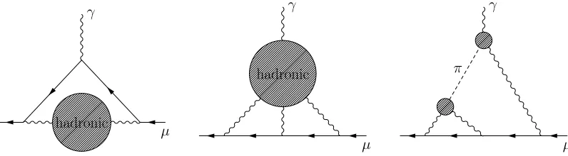
Figure 1. Left: Hadronic vacuum-polarization contribution to the gyromagnetic ratio of the muon. Middle:
Hadronic light-by-light scattering contribution.Right:Pion-pole part. Note that in the dispersive formulation the pion is onshell [6].
case in the timelike region areπ0→2e+2e−ande+e−→π0ℓ+ℓ−with a leptonℓ. Finally, the doubly virtual pion transition form factor in the spacelike region q2
1,q22 < 0 is probed, e.g., by reactions 2e− → π02e−ande+e− → π0e+e− where the pion can be produced via the fusion of two virtual
photons.
Like for any quantum-field theoretical quantity there are kinematical regions of the doubly virtual pion transition form factor that are not or not easily experimentally accessible, for instance ifq2
1 is spacelike andq2
2timelike. For the pion transition form factor there is an additional challenge: It is of ordere2, i.e. already small at the amplitude level. Observables where the pion transition form factor enters quadratically are therefore very much suppressed. As we will see below, dispersion theory offers a way to circumvent the direct determination of such small quantities.
In general, form factors describe the deviation from a pointlike behavior, i.e. for a pointlike pion the normalized transition form factorFπ0γ∗γ∗q21,q22/Fπ0γ∗γ∗(0,0) would be unity, independent of the virtualitiesq2
1andq22of the electromagnetic currents. In other words, form factors encode the infor-mation about the composite structure of an object. Thus, from the point of view of hadron physics, the pion transition form factor tells us something about the intrinsic (quark-gluon) structure of the neutral pion. Yet there is a broader interest in this particular form factor beyond the motivation to explore the composite structure of strongly interacting matter. One promising way to look for physics beyond the standard model is to compare experimental results and corresponding standard-model calculations for selected observables where one can achieve high precision both on the experimental side and on the theoretical (standard model) side. A clear (statisticallysignificant) deviation between theory (standard model) and experiment would point towards an additional impact on the respective observable from physical effects beyond the standard model. For this endeavor the gyromagnetic ratio of the muon provides a very promising observable [3, 4]; see also the presentations by B. Kubis, M. Procura, M. Knecht, and F. Jegerlehner in these workshop proceedings. The pion transition form factor is a crucial ingredient to improve the standard-model prediction for this quantity. We note in passing that also the rare decayπ0→e+e−is sensitive to the pion transition form factor and might have some potential to reveal effects from physics beyond the standard model; see [2, 5] and references therein.
At present, the largest uncertainty in the standard-model prediction for the gyromagnetic ratio of the muon resides in the so-called hadronic vacuum-polarization contribution depicted on the left hand side of figure 1. It turned out that a significant part of this contribution comes from hadronic physics
γ
µ hadronic
γ
µ hadronic
γ
µ π
Figure 1. Left: Hadronic vacuum-polarization contribution to the gyromagnetic ratio of the muon. Middle:
Hadronic light-by-light scattering contribution.Right:Pion-pole part. Note that in the dispersive formulation the pion is onshell [6].
below 2 GeV. Thus perturbative QCD cannot be used to calculate this contribution. Also the non-perturbative regime of the strong interaction is probed here. On the other hand, a phenomenological
hadronic model might produce a number for the hadronic vacuum-polarization contribution but not a serious theory uncertainty estimate. Given that one wants to test the standard model and not the quality of a phenomenological hadronic model, one has to resort to methods firmly based on QCD or quantum field theory in general. Fortunately, the hadronic vacuum-polarization contribution can be directly related via dispersion theory to the cross sectione+e−→hadrons [3]. Thus, instead of modeling this
contribution with not determinable accuracy one can use data with experimentally known accuracy. This interrelation between the hadronic vacuum-polarization contribution and hadronic data has triggered significant experimental activities as can be deduced from numerous presentations in these proceedings. As a consequence of these on-going activities it can be expected that the uncertainty in the standard-model prediction originating in the hadronic vacuum-polarization contribution will be significantly reduced in the near future. This development moves the focus to the next hadronic contribution to the gyromagnetic ratio of the muon: the hadronic light-by-light scattering contribution depicted in the middle of figure 1. So far, the size of this contribution has been determined by hybrids of hadronic and quark models and attaching a rather conservative and therefore big model uncertainty to the results [3, 4].
Given the ongoing experimental activities to improve on the direct determination of the gyromag-netic ratio of the muon and on the input for the hadronic vacuum-polarization contribution, it is high time to improve also on the standard-model prediction for the hadronic light-by-light scattering con-tribution including a reliable uncertainty estimate. In [6–9] a dispersive framework has been proposed to address the hadronic light-by-light scattering contribution. This framework is based on data and fundamental principles of quantum field theory, QED and QCD.It is expected that the numerically most important part of the hadronic light-by-light scattering contribution comes from processes where the hadronic blob in the middle diagram of figure 1 is replacedby the lowest-mass hadronic state, the pion. Such a process, the “pion-pole term”, is sketched by the right diagram of figure 1. Other im-portant parts of the hadronic light-by-light scattering contribution come from processes where the hadronic blob in the middle diagram of figure 1 is replaced by anη- orη′-meson or by a pair of pions.
These processes are discussed in the contributions of B. Kubis and M. Procura. The central quantity that needs to be determined for the calculation of the pion-pole term is just the doubly virtual pion transition form factor. Note that in the dispersive framework the pion in figure 1 is onshell while the photons in the loops can have arbitrary virtuality; see the corresponding discussion in [6]. This matches with the definition (1) of the pion transition form factor where the pion is an external, i.e. physical state.
2 Dispersion theory
The ambition is to determine via dispersion theory and experimental data the pion-pole term, which constitutes an important part of the hadronic light-by-light scattering contribution to the gyromagnetic ratio of the muon. The aim is a numerical value for this contributionandan associated reliable theory uncertainty estimate. Using dispersion theory provides the advantage that this framework and therefore also the uncertainty estimate is solely based on QED, QCD and fundamental principles of quantum field theory. In turn quantum field theory constitutes the basis of the standard model. Thus an uncertainty estimate based on this data-driven dispersive approach can truly be regarded as a standard-model uncertainty estimate.
Transitions from any initial to any final state can be encodedin theS-matrix. Demanding that the total probability to obtain an arbitrary final state must be 1(probabilistic interpretation of quantum mechanics) leads to the unitarity condition
S S†=1. (3)
TheS-matrix contains the possibility that no interaction has taken place. This trivial part can be split offby introducing theT-matrix via S =: 1+iT. The unitarity condition (3) provides a profound relation forT, the optical theorem:
2 ImT =T T†. (4)
Note that this is a matrix equation. For an initial stateAand a final stateBthe relation (4) reads 2 ImTA→B=
X
TA→XTX†→B. (5)
The locality requirement of relativistic quantum field theory demands that scattering amplitudes consist of polynomials (from thelocalinteraction vertices), propagators and integrals thereof. The poles of the propagators are related to physical states. Consequently scattering amplitudes are analytic except for poles and cuts, which have a one-to-one correspondence to physical intermediate states. Schematically this can be expressed via thedispersion relation1
T(s)=1
π
∞
−∞
ds′ ImT(s′)
s′−s−iǫ. (6)
Thus, based on analyticity, one can obtain the whole amplitude from its imaginary part. On the other hand, based on unitarity, one can obtain the imaginary part of the amplitude from other amplitudes on account of (5).2
One situation where such a framework is of particular importance is the case whereTA→B is
very small. For instance, the pion transition form factor is doubly suppressed by the electromagnetic coupling constante. Here one might identifyAwithγ∗andBwithγ∗π0. Because of the overwhelming
strength of the strong interaction the sum of intermediate statesX in (5) is dominated by hadrons. Thus, while the amplitudeTA→Bis of ordere2, the amplitudesTA→XandTX→Bare both of ordere, i.e.
less suppressed and therefore more easily accessible by experiment.
Of course, there are practical limitations for such a dispersive reconstruction of amplitudes. First of all, one formally needs to know ImT in (6) up to infinitely large energies. This can never be achieved by experiment. Second, it seems that it is necessary to know/measure the amplitudesTA→X andTX→Bforallintermediate statesX. Both problems can be tamed by subtracted dispersion relations
and by restricting the attention to not too large values of|s|in (6). In principle, a systematic framework to determine hadronic scattering amplitudes at very low energies is chiral perturbation theory. How-ever, it turned out that the energy regime covered by chiral perturbation theory is not large enough to provide a reliable calculational framework for the pion-pole term (right diagram in figure 1). The dispersive framework is in practice also restricted to low energies, but the results remain reliable in a regime that is larger than the one covered by chiral perturbation theory.
As already spelled out, one can utilize subtracted dispersion relations to suppress the influence of the largely unknown high-energy region and to restrict the sum over all intermediate statesXto a 1In reality a scattering amplitude depends on several kinematical variables. For instance a partial-wave decomposition might boil it down to a one-variable function.
Transitions from any initial to any final state can be encodedin theS-matrix. Demanding that the total probability to obtain an arbitrary final state must be 1(probabilistic interpretation of quantum mechanics) leads to the unitarity condition
S S†=1. (3)
TheS-matrix contains the possibility that no interaction has taken place. This trivial part can be split offby introducing theT-matrix via S =: 1+iT. The unitarity condition (3) provides a profound relation forT, the optical theorem:
2 ImT =T T†. (4)
Note that this is a matrix equation. For an initial stateAand a final stateBthe relation (4) reads 2 ImTA→B=
X
TA→XTX†→B. (5)
The locality requirement of relativistic quantum field theory demands that scattering amplitudes consist of polynomials (from thelocalinteraction vertices), propagators and integrals thereof. The poles of the propagators are related to physical states. Consequently scattering amplitudes are analytic except for poles and cuts, which have a one-to-one correspondence to physical intermediate states. Schematically this can be expressed via thedispersion relation1
T(s)=1
π
∞
−∞
ds′ ImT(s′)
s′−s−iǫ. (6)
Thus, based on analyticity, one can obtain the whole amplitude from its imaginary part. On the other hand, based on unitarity, one can obtain the imaginary part of the amplitude from other amplitudes on account of (5).2
One situation where such a framework is of particular importance is the case where TA→B is
very small. For instance, the pion transition form factor is doubly suppressed by the electromagnetic coupling constante. Here one might identifyAwithγ∗andBwithγ∗π0. Because of the overwhelming
strength of the strong interaction the sum of intermediate statesX in (5) is dominated by hadrons. Thus, while the amplitudeTA→Bis of ordere2, the amplitudesTA→XandTX→Bare both of ordere, i.e.
less suppressed and therefore more easily accessible by experiment.
Of course, there are practical limitations for such a dispersive reconstruction of amplitudes. First of all, one formally needs to know ImT in (6) up to infinitely large energies. This can never be achieved by experiment. Second, it seems that it is necessary to know/measure the amplitudesTA→X andTX→Bforallintermediate statesX. Both problems can be tamed by subtracted dispersion relations
and by restricting the attention to not too large values of|s|in (6). In principle, a systematic framework to determine hadronic scattering amplitudes at very low energies is chiral perturbation theory. How-ever, it turned out that the energy regime covered by chiral perturbation theory is not large enough to provide a reliable calculational framework for the pion-pole term (right diagram in figure 1). The dispersive framework is in practice also restricted to low energies, but the results remain reliable in a regime that is larger than the one covered by chiral perturbation theory.
As already spelled out, one can utilize subtracted dispersion relations to suppress the influence of the largely unknown high-energy region and to restrict the sum over all intermediate statesXto a 1In reality a scattering amplitude depends on several kinematical variables. For instance a partial-wave decomposition might boil it down to a one-variable function.
2Note that this is a schematic, oversimplified discussion of dispersion theory. For the full-fledged formalism we refer to[1] and references therein.
manageable amount. For simplicity we specify the scattering amplitude to some extent by studying a transition form factorFBC related to�C|j|B� where jdenotes a quark current. To make contact with the previous formulae one should identify schematicallyAfrom (5) with jandBfrom (5) with B C. Furthermore we assume that the lowest-mass intermediate states Xare given by 2-pion states. Schematically a twice-subtracted dispersion relation is given by
FBC(s)=FBC(0)+F′BC(0)s+s
2
π
∞
4m2 π
ds′TBC∗ ππ(s′)Fππ(s′)
(s′)2(s′−s−iǫ)+. . . . (7)
The general idea is to obtain the subtraction constantsFBC(0),F′BC(0) from data and/or chiral pertur-bation theory and the amplitudesTBCππandFππfrom data or other dispersion relations. Note that the s′integral starts at the threshold of the 2-pion states. The dots in (7) refer to other intermediate states
different from 2-pion states. These additional states produce correspondings′-integrals. It is crucial
to understand that these additional states are heavier and therefore contribute only for large values of s′. We want to know the transition form factorFBCfor small values of|s|. Then all contributions from
large values ofs′are highly suppressed by∼(1/s′)3. This should be compared to the unsubtracted
dispersion relation (6) where there is only a 1/s′ suppression of the high-energy part. Subtractions
help to focus on the low-energy information. The price to pay are the subtraction constants that need to be obtained from other sources. In addition, the high-energy behavior of the amplitude is mod-ified. Typically general constraints from scattering theory and asymptotic QCD are at odds with a polynomial growth of the scattering amplitudes. Thus especially for the uncertainty estimates it must be carefully monitored to which extent an incorrect high-energy behavior influences the results for observables.
In (7) all the quantities that we do not know so well — the contributions from other intermediate states and the amplitudesTBCππ(s′) andFππ(s′) for large values ofs′— are highly suppressed. In practice one can introduce a high-energy cutoffbelow which we trust our amplitudesTBCππ(s′) and Fππ(s′). Here “trust” means that we can quantify the uncertaintiesof these amplitudes. Varying this cutoffin a reasonable range and exploring different high-energy extrapolations of the amplitudes allows one to quantify the overall uncertainty of the quantity of interest, namelyFBC(s) for low values of|s|. In practice, √|s|should be smaller than about 1 GeV, where, for instance, the 4-pion continuum starts to become noticeable.
3 First results
For the pion transition form factor one might schematically identifyBwithγ∗ andCwithπin (7).
Thus one needs the amplitudeTγ∗3π and the pion vector form factorFππ. For both quantities one can set up again a dispersive framework. At low energies the relevant intermediate states are again 2-pion states. Thus the pion vector form factor can be determined from the 2-pion (p-wave) phase shift — and possibly a low-order polynomial accounting for not explicitly considered other intermediate states. These states cannot create a strongly varying function at low energies. Thus a low-order polynomial should be sufficient. The pion phase shifts have been determined from (dispersively improved) data by two different groups [10, 11]. The differences between the two analyses can be used as an uncertainty estimate for the input pion phase shift. The pion vector form factor is also experimentally very well known. It agrees fairly well with the dispersive reconstruction from the pion p-wave phase shift. The data can be used to pin down the low-order polynomial; see [12] for details.
correlations. In contrast, the 2-pion invariant masses (Mandelstam variables) depend on the 2-pion correlations, i.e. on the pion phase shifts. As already discussed, the pion phase shifts are under control [10, 11]. With this input dispersion theory can be used to determine the dependence ofTγ∗3π on the 2-pion invariant masses for any photon virtuality [1, 13]. Physically this accounts for pion rescattering and cross-channel rescattering. What remains to be determined is the dependence of the amplitude Tγ∗3π on the photon virtuality, i.e. on the genuine 3-pion correlations. Here “genuine” means the correlations not caused by a succession of cross-channel 2-pion correlations.
0.6 0.7 0.8 0.9 1.0 1.1
10-2 10-1
100 101 102 103
fit SND+BaBar
fit HLMNT
SND
BaBar
√
q2[GeV] σe
+e −→
3
π
[nb
]
Figure 2.Fit to the cross section
e+e−
→3π. Figure taken from [1]. There
is a tension between different data sets.
This causes a significant theory uncertainty in our calculations.
Starting from an amplitude that depends on several variables we have reduced the problem to the determination of a one-parameter function that accounts for the genuine 3-pion correlations. This can be achieved by fitting to a one-variable observable, namely to the energy dependence of the total cross section for the reactione+e−→3π. Physically it is known that 3 pions with the quantum numbers of
a photon are strongly correlated to theωandφmesons. Thus we parametrize our one-parameter fit function accordingly by dispersively improved Breit-Wigner functions and a polynomial. The quality of our fit can be inspected in figure 2.
0.5 0.6 0.7 0.8 0.9 1.0 1.1
10-3 10-2 10-1 100 101
102 SND
CMD2
√
q2[GeV]
σe
+e −→
π
0γ
[nb
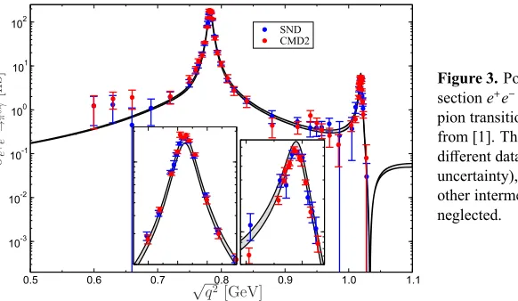
] Figure 3.Postdiction for the cross
sectione+e−→π0γ(probes the timelike pion transition form factor). Figure taken from [1]. Theory uncertainties from different data sets fore+e−→3π(main uncertainty), different pion phase shifts, other intermediate states than 2π
neglected.
be-correlations. In contrast, the 2-pion invariant masses (Mandelstam variables) depend on the 2-pion correlations, i.e. on the pion phase shifts. As already discussed, the pion phase shifts are under control [10, 11]. With this input dispersion theory can be used to determine the dependence ofTγ∗3π on the 2-pion invariant masses for any photon virtuality [1, 13]. Physically this accounts for pion rescattering and cross-channel rescattering. What remains to be determined is the dependence of the amplitude Tγ∗3π on the photon virtuality, i.e. on the genuine 3-pion correlations. Here “genuine” means the correlations not caused by a succession of cross-channel 2-pion correlations.
0.6 0.7 0.8 0.9 1.0 1.1
10-2 10-1 100 101 102 103 fit SND+BaBar fit HLMNT SND BaBar √
q2[GeV] σe +e −→ 3 π [nb ]
Figure 2.Fit to the cross section
e+e−
→3π. Figure taken from [1]. There
is a tension between different data sets.
This causes a significant theory uncertainty in our calculations.
Starting from an amplitude that depends on several variables we have reduced the problem to the determination of a one-parameter function that accounts for the genuine 3-pion correlations. This can be achieved by fitting to a one-variable observable, namely to the energy dependence of the total cross section for the reactione+e−→3π. Physically it is known that 3 pions with the quantum numbers of
a photon are strongly correlated to theωandφmesons. Thus we parametrize our one-parameter fit function accordingly by dispersively improved Breit-Wigner functions and a polynomial. The quality of our fit can be inspected in figure 2.
0.5 0.6 0.7 0.8 0.9 1.0 1.1
10-3 10-2 10-1 100 101
102 SND
CMD2
√
q2[GeV]
σe +e −→ π 0γ [nb
] Figure 3.Postdiction for the cross
sectione+e−→π0γ(probes the timelike pion transition form factor). Figure taken from [1]. Theory uncertainties from different data sets fore+e−→3π(main uncertainty), different pion phase shifts, other intermediate states than 2π
neglected.
The present status of our dispersive calculation of the pion transition form factor is that we have de-termined the singly virtual transition form factor in the timelike and spacelike region for momenta
be-low 1 GeV. The dispersive reconstruction of the doubly virtual pion transition form factor is presently investigated. In the timelike region the singly virtual transition form factor is directly related to the cross section for the reactione+e− → π0γ. Figure 3 shows that we have obtained an excellent
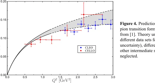
de-scription of this cross section. Our prediction for the singly virtual pion transition form factor in the spacelike region is shown in figure 4. We are looking forward to experimental cross-checks of our prediction.
0.0 0.5 1.0 1.5 2.0 2.5 3.0
0.00 0.05 0.10 0.15 0.20 CLEO CELLO
Q2[GeV2]
Q 2F π 0γ ∗γ ( − Q 2, 0) /e 2[G eV ]
Figure 4.Prediction for the space-like pion transition form factor. Figure taken from [1]. Theory uncertainties from different data sets fore+e−→3π(main uncertainty), different pion phase shifts, other intermediate states than 2π
neglected.
The final aim of our endeavor is to determine with a reliable (and hopefully small) uncertainty estimate the pion-pole term as one important part of the hadronic light-by-light scattering contribution to the standard-model prediction for the gyromagnetic ratio of the muon. Clearly the quality of our results hinges on the quality of the experimental input that we use. We will spend the rest of this presentation to spell out a wish list with interesting observables that could help to improve the input for the dispersive calculations and/or to further scrutinize our framework.
4 Interesting observables
It would improve the input for our dispersive framework [7], if (1) remaining ambiguities in the data for the cross sectione+e− →3πcould be resolved, (2) a Dalitz plot for the decayω→ 3πcould be
provided with the same accuracy as already achieved forφ→3π, (3) the cross section for the reaction γπ→2πcould be provided.
Cross-checks of our approach can be obtained by improved determinations of the transition form factorsω → π0e+e−andφ → π0e+e− in the respective full kinematically accessible Dalitz decay
regions.
4.1 Resolve ambiguities in the cross sectione+e−
→3π
As a matter of fact the various data sets for the cross section of the reactione+e−→3πare not fully
one of the two inlays) shows visible differences at theφpeak. For a more detailed discussion of all the uncertainties we refer to [1].
Some uncertainties of thee+e− → 3πcross section data and maybe discrepancies between the
data sets might be caused by the extrapolation of the actual 3-pion measurements to the full 4π an-gular coverage. In that context we note that the dispersive framework of [13] predicts the anan-gular distribution of the three pions for a given collision energy of thee+e−system, see also figure 5 below.
Such information might help for cross-checking the experimental acceptance corrections and for the extrapolation to the full 4πangle.
4.2 Dalitz plotω→3π
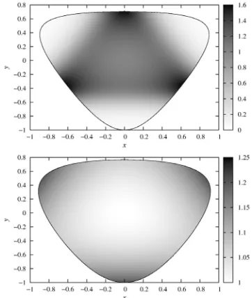
The amplitudeTγ∗3πdiscussed in section 3 is also probed in the decays of vector mesonsVto three pions. Here the virtuality of the photon (better to say: of the electromagnetic current) is fixed to the respective mass of the vector meson. If one utilizes a once subtracted dispersion relation, then one can predict the Dalitz decay distribution of the decayV → 3π; see the left hand side of figure 5. The subtraction constant is fixed by the corresponding decay width. For the decay φ → 3πit turns out that the data have such an excellent quality — see the top right panel of figure 5 — that a better description of the data can be achieved by a twice subtracted dispersion relation [13]. The two subtraction constants are determined by a combined fit to thedecay width and the distribution itself. As we will argue now, we would like to know the values of these subtraction constant pair also for the decayω→3πand for the reactionγπ→2π.
Figure 5.Top, left:Dispersive calculation of the Dalitz decay distribution forφ→3π. Figure taken from [13]. Top, right:KLOE data forφ →3πwith comparable quality. Figure taken from [14]. Bottom, left:Dispersive
calculation of the Dalitz decay distribution forω→3π. Figure taken from [13].Bottom, right:Missing, i.e. no
data with comparable quality forω→3π.
one of the two inlays) shows visible differences at theφpeak. For a more detailed discussion of all the uncertainties we refer to [1].
Some uncertainties of thee+e− → 3πcross section data and maybe discrepancies between the
data sets might be caused by the extrapolation of the actual 3-pion measurements to the full 4π an-gular coverage. In that context we note that the dispersive framework of [13] predicts the anan-gular distribution of the three pions for a given collision energy of thee+e−system, see also figure 5 below.
Such information might help for cross-checking the experimental acceptance corrections and for the extrapolation to the full 4πangle.
4.2 Dalitz plotω→3π
The amplitudeTγ∗3π discussed in section 3 is also probed in the decays of vector mesonsV to three pions. Here the virtuality of the photon (better to say: of the electromagnetic current) is fixed to the respective mass of the vector meson. If one utilizes a once subtracted dispersion relation, then one can predict the Dalitz decay distribution of the decayV → 3π; see the left hand side of figure 5. The subtraction constant is fixed by the corresponding decay width. For the decayφ → 3πit turns out that the data have such an excellent quality — see the top right panel of figure 5 — that a better description of the data can be achieved by a twice subtracted dispersion relation [13]. The two subtraction constants are determined by a combined fit to thedecay width and the distribution itself. As we will argue now, we would like to know the values of these subtraction constant pair also for the decayω→3πand for the reactionγπ→2π.
Figure 5.Top, left:Dispersive calculation of the Dalitz decay distribution forφ→3π. Figure taken from [13]. Top, right:KLOE data forφ →3πwith comparable quality. Figure taken from [14]. Bottom, left:Dispersive
calculation of the Dalitz decay distribution forω→3π. Figure taken from [13].Bottom, right: Missing, i.e. no
data with comparable quality forω→3π.
In [1] we have determined the amplitudeTγ∗3πfor arbitrary photon virtualities from a once sub-tracted dispersion relation. Since the considered intermediate states, cf. (5), are 2-pion states, the
variable in the dispersion integral is one of the 2-pion invariant masses, not the 3-pion invariant mass. However, the subtraction constant depends on the 3-pion invariant mass, i.e. on the photon virtuality. As described in the previous section we have related this dependence of the subtraction constant to the cross section of the reactione+e−→3π.
If one could determine the amplitudeTγ∗3πfrom a twice instead of a once subtracted dispersion relation, then the unknown high-energy parts would be further suppressed, cf. the discussion around (7). In turn this would reduce our theory uncertainty. But then we would need to get an idea about the dependence of the second subtraction constant on the photonvirtuality. So far, we only know the value at one point, where the virtuality coincides with theφmass. As discussed above, this information comes from the high-quality Dalitz decay distributionφ→3π. If we could deduce the corresponding second subtraction constant also from a comparable high-quality Dalitz decay distributionω → 3π and from the cross section of the reactionγπ→2π, then one could interpolate the dependence of this second subtraction constant on the photon virtuality from zero up to theφmass.
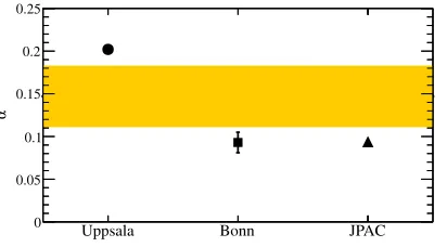
Unfortunately there exists noω → 3πDalitz plot with an accuracy comparable to the achieve-ments forφ→3π. Actually until recently there was no experimental indication at all that the pions in the decayω→3πshow any final-state interaction. Experimental data could not distinguish between pure phase space and pion rescattering. In [15] first steps beyond pure phase space are documented. Following [13] a parameterαhas been introduced to parametrize for the Dalitz plot ofω→ 3πthe main deviation from pure phase space. A vanishingαwould signal the absence/smallness of pion rescattering. This possibility has been ruled out by [15]; see figure 6. The experimental value ofα is definitely different from zero and lies in the ballpark of recent theory predictions. The dispersive
prediction is labeled by “Bonn” in figure 6. The future experimental challenge is to produce anα value with a better accuracy than the one obtained by dispersion theory. Only with such a quality the parameters of a twice subtracted dispersion relation could be pinned down.
Figure 6.ω→3π— first steps beyond pure phase space. Experimental verification (yellow band) of a Dalitz plot shape beyond pure phase space, i.e.
α0. Also shown is a comparison to recent theory predictions forα. “Uppsala” refers to [16], “Bonn” to [13], and “JPAC” to [17]. Figure taken from [15].
4.3 Cross sectionγ+π→ 2π
As already noted a remaining piece of information should come from the cross section of the reaction γ+π →2π. This could be measured with a pion beam by a Primakoffreaction, for instance by the
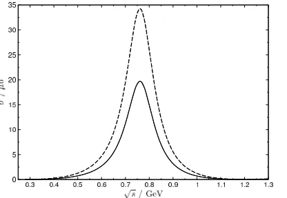
figure 7 one can use the whole energy range up to theρ-meson mass to pin down the value of the anomaly.
Figure 7.Prediction of the cross sectionγ+π→2π
based on dispersion theory.Solid line:prediction from anomaly;dashed line:size of anomaly scaled up by about 30% . Figure taken from [18].
Concerning our amplitudeTγ∗3πwe use the chiral anomaly to pin down a subtraction constant. A better procedure would be to use the corresponding physical quantity that includes chiral corrections caused by the non-vanishing light quark masses.3 With data from the reactionγ+π→2πor maybe from lattice QCD [19] one could improve on this aspect. With higher-quality data at hand one could even use a twice subtracted dispersion relation and obtain additional knowledge and lower theory uncertainties as pointed out in the previous subsection.
4.4 Transition form factorω→π0ℓ+
ℓ−
The decay of a vector meson toπ0ℓ+ℓ−, whereℓdenotes a lepton, probes a transition form factor that
has the same quantum numbers as the pion transition form factor. Consequently the same dispersive framework can be used to determine the form factors of these electromagnetic transitions from a vector meson to a pion [12]. Experimentally one has to determine the differential decay width as a function of the dilepton mass.
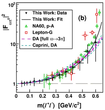
For the decayω →π0µ+µ−the dispersive results deviate significantly from the data obtained by
the NA60 collaboration [20, 21]. On the other hand, recent data for the decayω →π0e+e−obtained
by the A2 collaboration [22] lie right on top of the dispersive prediction; see figure 8.
If one just looks at the various data sets and their error barsin figure 8 — without the theory lines that might misguide the eye — then one might still get the impression that the data are not in complete contradiction to each other, though the trends differ. Yet it is remarkable that no hadronic theory has been able to fully explain the NA60 data and according to [23] part of these data disagree with general information obtained from QCD and quantum field theory. Thusit would be very illuminating to have additional data that could help to resolve the tension between NA60 on the one side and the dispersive calculation and A2 on the other side.
From a dispersive point of view the input for the transition form factor probed byω → π0ℓ+ℓ− comes from the amplitudeω3π; the reader may just replaceB→ωandC→πin (7). The amplitude ω3πcan also be determined dispersively [13], but it would be good to have an experimental cross-check on this input for the transition form factor. Thus we repeat our call from subsection 4.2 for a high-quality Dalitz plot for the decayω→3π. The situation is somewhat different if one replacesω byφ, as we will discuss next.
figure 7 one can use the whole energy range up to theρ-meson mass to pin down the value of the anomaly.
Figure 7.Prediction of the cross sectionγ+π→2π
based on dispersion theory.Solid line:prediction from anomaly;dashed line:size of anomaly scaled up by about 30% . Figure taken from [18].
Concerning our amplitudeTγ∗3πwe use the chiral anomaly to pin down a subtraction constant. A better procedure would be to use the corresponding physical quantity that includes chiral corrections caused by the non-vanishing light quark masses.3 With data from the reactionγ+π→2πor maybe from lattice QCD [19] one could improve on this aspect. With higher-quality data at hand one could even use a twice subtracted dispersion relation and obtain additional knowledge and lower theory uncertainties as pointed out in the previous subsection.
4.4 Transition form factorω→π0ℓ+
ℓ−
The decay of a vector meson toπ0ℓ+ℓ−, whereℓdenotes a lepton, probes a transition form factor that
has the same quantum numbers as the pion transition form factor. Consequently the same dispersive framework can be used to determine the form factors of these electromagnetic transitions from a vector meson to a pion [12]. Experimentally one has to determine the differential decay width as a function of the dilepton mass.
For the decayω→ π0µ+µ−the dispersive results deviate significantly from the data obtained by
the NA60 collaboration [20, 21]. On the other hand, recent data for the decayω→π0e+e−obtained
by the A2 collaboration [22] lie right on top of the dispersive prediction; see figure 8.
If one just looks at the various data sets and their error barsin figure 8 — without the theory lines that might misguide the eye — then one might still get the impression that the data are not in complete contradiction to each other, though the trends differ. Yet it is remarkable that no hadronic theory has been able to fully explain the NA60 data and according to [23] part of these data disagree with general information obtained from QCD and quantum field theory. Thusit would be very illuminating to have additional data that could help to resolve the tension between NA60 on the one side and the dispersive calculation and A2 on the other side.
From a dispersive point of view the input for the transition form factor probed byω → π0ℓ+ℓ− comes from the amplitudeω3π; the reader may just replaceB→ωandC→πin (7). The amplitude ω3πcan also be determined dispersively [13], but it would be good to have an experimental cross-check on this input for the transition form factor. Thus we repeat our call from subsection 4.2 for a high-quality Dalitz plot for the decayω→3π. The situation is somewhat different if one replacesω byφ, as we will discuss next.
3The chiral-anomaly prediction is based on the chiral limit.
Figure 8.The electromagnetic form factor of the transitionωtoπ0from various experiments and theory approaches. The figure is adopted from the recent work [22] of the A2 collaboration and “This work” refers to it. The magenta lines show the dispersive calculation from [12].
We note in passing that in principle the cross section for the reactione+e−→π0ωprobes the very
same transition form factor, albeit in a kinematically different regime. For the energies relevant for this reaction one cannot expect that the relevant intermediate states, cf. (5), are just the 2-pion states. Thus this reaction cannot be used to scrutinize the present dispersive framework, which applies to reaction energies below 1 GeV, not above.
4.5 Transition form factorφ→π0e+e−
inρ-peak region
Another closely related transition form factor is probed by the decayφ → π0ℓ+ℓ−. A dispersive
prediction has been provided in [12], see figure 9. The input for the dispersive calculation is provided by the amplitudeφ3π, which can also be determined dispersively. The latter has been cross-checked successfully against high-quality data on the Dalitz plotφ → 3π[13]. Thus a very firm prediction forφ → π0ℓ+ℓ−has been obtained. Of course, it would be interesting to see if one finds for theφa deviation between data and theory that resembles the deviation between the NA60 data and theory for theωcase.
In contrast to the decayω → π0ℓ+ℓ− there is a resonance in the region that is kinematically
allowed for theφ decay — the ρmeson. Of course, most discriminative power between various theory approaches is achieved around the resonance peak, where the differential decay rate turns
large. Recently first data on the differential decay width forφ→ π0e+e−have been published by the KLOE-2 collaboration [24] and the corresponding transition form factor has been extracted; see the right hand side of figure 9. So far, the data are restricted to the region below theρ-meson peak and do not point to a significant disagreement between theory and experiment. But given the puzzle for theω transition form factor it would be highly desirable to explore the full kinematically accessible range of theφ→π0e+e−decay.
0 0.1 0.2 0.3 0.4 0.5 0.6 0.7 0.8 1
10 100
√s [GeV]
|
Fφ
π
0
(
s
)
|
2
VMD
f1(s) =aΩ(s)
once subtractedf1(s)
twice subtractedf1(s)
[GeV] 2 q
0 0.1 0.2 0.3 0.4 0.5 0.6
2)|
2
(q *γ
0π
φ
|F
1 10
Figure 9.Left:Prediction for the electromagnetic form factor of the transitionφtoπ0based on dispersion theory
[12]. The full calculation is shown by the yellow band. The complete kinematically allowed region for the decay
φ→π0e+e−is shown. Right:Extraction of the same form factor from KLOE-2 data in the low-energy region.
The yellow band from the plot on the left hand side translates here to the middle curve. Figure taken from [24].
Acknowledgments:The speaker (SL) thanks the organizers for an inspiring workshop in a very
enjoyable atmosphere. He also thanks P. Adlarson, S. Damjanovic, L. Heijkenskjöld, A. Kup´s´c, V.
Metag, P. Salabura, and H. Specht for many illuminating discussions. This work has been supported by
the project “Study of Strongly Interacting Matter” (HadronPhysics3, Grant Agreement No. 283286)
under the 7th Framework Program of the EU.
References
[1] M. Hoferichter, B. Kubis, S. Leupold, F. Niecknig and S. P. Schneider, Eur. Phys. J. C74, 3180
(2014)
[2] E. Czerwi´nski, S. Eidelman, C. Hanhart, B. Kubis, A. Kup´s´c, S. Leupold, P. Moskal and S. Schad-mand, “MesonNet Workshop on Meson Transition Form Factors,” arXiv:1207.6556 [hep-ph].
[3] F. Jegerlehner and A. Nyffeler, Phys. Rept.477, 1 (2009)
[4] J. Bijnens and J. Prades, Mod. Phys. Lett. A22, 767 (2007)
[5] T. Husek and S. Leupold, Eur. Phys. J. C75, 586 (2015)
[6] G. Colangelo, M. Hoferichter, M. Procura and P. Stoffer, JHEP1409, 091 (2014)
[7] G. Colangelo, M. Hoferichter, B. Kubis, M. Procura and P.Stoffer, Phys. Lett. B738, 6 (2014)
[8] G. Colangelo, M. Hoferichter, M. Procura and P. Stoffer, JHEP1509, 074 (2015)
[9] G. Colangelo, M. Hoferichter, M. Procura and P. Stoffer, arXiv:1701.06554 [hep-ph].
[10] B. Ananthanarayan, G. Colangelo, J. Gasser and H. Leutwyler, Phys. Rept.353, 207 (2001)
[11] R. García-Martín, R. Kaminski, J. R. Peláez, J. Ruiz de Elvira and F. J. Ynduráin, Phys. Rev. D´
0 0.1 0.2 0.3 0.4 0.5 0.6 0.7 0.8 1
10 100
√s [GeV]
|
Fφ
π
0
(
s
)
|
2
VMD
f1(s) =aΩ(s)
once subtractedf1(s)
twice subtractedf1(s)
[GeV] 2 q
0 0.1 0.2 0.3 0.4 0.5 0.6
2)|
2
(q *γ
0π
φ
|F
1 10
Figure 9.Left:Prediction for the electromagnetic form factor of the transitionφtoπ0based on dispersion theory
[12]. The full calculation is shown by the yellow band. The complete kinematically allowed region for the decay
φ→π0e+e−is shown. Right:Extraction of the same form factor from KLOE-2 data in the low-energy region.
The yellow band from the plot on the left hand side translates here to the middle curve. Figure taken from [24].
Acknowledgments: The speaker (SL) thanks the organizers for an inspiring workshop in a very
enjoyable atmosphere. He also thanks P. Adlarson, S. Damjanovic, L. Heijkenskjöld, A. Kup´s´c, V.
Metag, P. Salabura, and H. Specht for many illuminating discussions. This work has been supported by
the project “Study of Strongly Interacting Matter” (HadronPhysics3, Grant Agreement No. 283286)
under the 7th Framework Program of the EU.
References
[1] M. Hoferichter, B. Kubis, S. Leupold, F. Niecknig and S. P. Schneider, Eur. Phys. J. C74, 3180
(2014)
[2] E. Czerwi´nski, S. Eidelman, C. Hanhart, B. Kubis, A. Kup´s´c, S. Leupold, P. Moskal and S. Schad-mand, “MesonNet Workshop on Meson Transition Form Factors,” arXiv:1207.6556 [hep-ph].
[3] F. Jegerlehner and A. Nyffeler, Phys. Rept.477, 1 (2009)
[4] J. Bijnens and J. Prades, Mod. Phys. Lett. A22, 767 (2007)
[5] T. Husek and S. Leupold, Eur. Phys. J. C75, 586 (2015)
[6] G. Colangelo, M. Hoferichter, M. Procura and P. Stoffer, JHEP1409, 091 (2014)
[7] G. Colangelo, M. Hoferichter, B. Kubis, M. Procura and P.Stoffer, Phys. Lett. B738, 6 (2014)
[8] G. Colangelo, M. Hoferichter, M. Procura and P. Stoffer, JHEP1509, 074 (2015)
[9] G. Colangelo, M. Hoferichter, M. Procura and P. Stoffer, arXiv:1701.06554 [hep-ph].
[10] B. Ananthanarayan, G. Colangelo, J. Gasser and H. Leutwyler, Phys. Rept.353, 207 (2001)
[11] R. García-Martín, R. Kaminski, J. R. Peláez, J. Ruiz de Elvira and F. J. Ynduráin, Phys. Rev. D´
83, 074004 (2011)
[12] S. P. Schneider, B. Kubis and F. Niecknig, Phys. Rev. D86, 054013 (2012)
[13] F. Niecknig, B. Kubis and S. P. Schneider, Eur. Phys. J. C72, 2014 (2012)
[14] A. Aloisioet al.[KLOE Collaboration], Phys. Lett. B561, 55 (2003) Erratum: [Phys. Lett. B 609, 449 (2005)]
[15] P. Adlarsonet al.[WASA-at-COSY Collaboration], B. Kubis, S. Leupold, arXiv:1610.02187
[nucl-ex].
[16] C. Terschlüsen, B. Strandberg, S. Leupold and F. Eichstädt, Eur. Phys. J. A49, 116 (2013)
[17] I. V. Danilkin, C. Fernández-Ramírez, P. Guo, V. Mathieu, D. Schott, M. Shi and A. P.
Szczepa-niak, Phys. Rev. D91, 094029 (2015)
[18] M. Hoferichter, B. Kubis and D. Sakkas, Phys. Rev. D86, 116009 (2012)
[19] R. A. Briceño, J. J. Dudek, R. G. Edwards, C. J. Shultz, C.E. Thomas and D. J. Wilson, Phys.
Rev. D93, 114508 (2016)
[20] R. Arnaldiet al.[NA60 Collaboration], Phys. Lett. B677, 260 (2009)
[21] R. Arnaldiet al.[NA60 Collaboration], Phys. Lett. B757, 437 (2016)
[22] P. Adlarsonet al., arXiv:1609.04503 [hep-ex].
![Figure 9. Left: Prediction for the electromagnetic form factor of the transition φ to π0 based on dispersion theory[12]](https://thumb-us.123doks.com/thumbv2/123dok_us/8067388.1345169/12.482.39.427.79.301/figure-left-prediction-electromagnetic-factor-transition-dispersion-theory.webp)
