Article
Effects of Structure from Motion Data density,
interpolation method and grid size on micro
topography Digital Terrain Model accuracy
Francisco Agüera-Vega 1,*, Marta Agüera-Puntas 1, Patricio Martínez-Carricondo 1,2, Francesco Mancini 3 and Fernando Carvajal 1
1 Department of Engineering, Mediterranean Research Center of Economics and Sustainable Development
(CIMEDES), University of Almería (Agrifood Campus of International Excellence, ceiA3). La Cañada de San Urbano, s/n. 04120 Almería, Spain; [email protected] (M.A-P.); [email protected] (F.C-R.); [email protected] (P.M.C.)
2 Peripheral Service of Research and Development based on drones, University of Almeria. La Cañada de
San Urbano, s/n. 04120 Almería, Spain
3 Department of Engineering “Enzzo Ferrari”, University of Modena and Reggio Emilia, Italy.
[email protected] (F.M.)
* Correspondence: [email protected] (F.A-V.)
Abstract: The objective of this study is to evaluate the effects of the 3D point cloud density derived from unmanned aerial vehicle (UAV) photogrammetry and structure from motion (SfM) and multi-view stereopsis (MVS) techniques, the interpolation method for generating a digital terrain model (DTM), and the resolution (grid size) of the derived DTM on the accuracy of estimated heights in small areas, where a very accurate high spatial resolution is required. A UAV-photogrammetry project was carried out on a bare soil of 13 × 13 m with a rotatory wing UAV at 10 m flight altitude (equivalent ground sample distance = 0.4 cm). The 3D point cloud was derived, and five sample replications representing 1, 2, 3, 4, 5, 10, 15, 20, 30, 40, 50, 60, 70, 80 and 90% of the original cloud were extracted to analyze the effect of cloud density on DTM accuracy. For each of these samples, DTMs were derived using four different interpolation methods (Inverse Distance Weighted (IDW), Multiquadric Radial Basis Function (MRBF), Kriging (KR), and Triangulation with Linear Interpolation (TLI)) and 15 DTM grid size (GS) values (20, 15, 10, 9, 8, 7, 6, 5, 4, 3, 2, 1, 0.67, 0.5, and 0.4 cm). Then, 675 DTMs were analyzed. The results showed, for each interpolation method and each density, an optimal GS value (most of the cases equal to 1 cm) for which the Root Mean Square Error (RMSE) is minimum. IDW was the interpolator which yielded best accuracies for all combination of densities and GS. Its RMSE, considering the raw cloud, was 1.054 cm. The RMSE increased 3% when a point cloud with 80% extracted from the raw cloud was used to generate the DTM. When the point cloud included the 40% of the raw cloud, RMSE increased 5%. For densities lower than 15%, RMSE increased exponentially (45% for 1% of raw cloud). The grid size minimizing RMSE for densities of 20% or higher was 1 cm, which represents 2.5 times the ground sample distance of the pictures used for developing the photogrammetry project.
Keywords: UAV-photogrammetry; digital surface model; Structure from Motion; microtopography
1. Introduction
A Digital Elevation Model (DEM) represents a mathematical expression of an object. It is usually used for describing terrains, giving its elevations without considering the vegetation or man-made features. It plays an important role in applications related to terrain modeling, hydrological modeling, or landscape evolution due erosion process [1–3]. When a high scale is required, it is very important to count with a point cloud which yields a high resolution and high quality DEM.
Furthermore, Unmanned Aerial Vehicles (UAVs) can catch data which, combined with remote sensing techniques, provide 3D models and orthophotographs with a high spatial and temporal resolution [3]. These products are very useful for landscape monitoring: reconstruction of extreme topography [4], precision agriculture [5–7], landslide monitoring [8], or erosion assessment [9]. All these applications require very high spatial resolution and very high accuracy.
The integration of photogrammetry and computer vision has provided the Structure from Motion (SfM) technique, from which is possible to collect images from different heights and in different directions, with greater flexibility and high quality results [10,11]. SfM solves automatically the geometry of the scene and the camera positions and orientation, without the need to specify a priori a network of targets which have known 3D positions [12–14]. The multi-view stereopsis (MVS) technique has been incorporated into SfM, and it allows to derive the 3D structure from overlapping photography acquired from multiples angles. Furthermore, the Scale Invariant Feature Transform (SIFT) operator has been shown to be one of the most robust for key-point detection for generating 3D point clouds from 2D photographs [15,16]. All this has led to the so-called UAV-photogrammetry, which consists of taking pictures from a non-metric camera mounted on a UAV to obtain a 3D point cloud representing the studied object.
Having an accurate 3D point cloud, several factors affect the accuracy of the DEM: density and distribution of point cloud, grid resolution, and interpolation method to generate the DEM. UAV-photogrammetry is able to generate high 3D point densities. However, this must be accompanied by proper system for data storage, data processing and manipulation of large volumes of data. High 3D point densities and high DEM grid resolution imply long processing time both in point cloud generation and DEM generation. So, reductions of such high point densities contribute to reduce the cost of data acquisition and data computation [17]. Although reduction in point cloud densities and DEM grid size reduction are expected to have direct effects on DEM characteristics, if those effects are not significant for a given application, this could result in saving in data acquisition and processing costs by a balance between them.
Although there are no published works studying these effects on data generated from UAV-photogrammetry, there are some on a 3D cloud point generated with terrestrial LiDAR technology. Anderson et al. [18] reduced the original LiDAR point cloud, resulting in data sets with 50%, 25%, 10%, 5% and 1% of their original densities. Furthermore, they used two interpolators (inverse distance weighting (IDW) and ordinary kriging) to generate the DEM. Study of the errors concluded that LiDAR data sets could withstand substantial data reductions yet maintain adequate accuracy for elevation predictions, and that simple interpolation approaches such as IDW could be sufficient for generating the DEM. Liu et al. [19] explored the effect of point cloud density acquired with LiDAR and examined the scope for data volume reduction without affecting the efficiency in data storage and processing. They concluded that, although datasets could be reduced increasing the efficiency of DEM generation, the maximum level of data reduction depends on the original data density, interpolation method, DEM grid size, and terrain characteristics. Liu et al. [20] explored the effects of LiDAR data density on the accuracy of DEMs and examined how much a set of this data can be reduced while maintaining adequate accuracy for DEM generation. They concluded that data reduction mitigates the data redundancy and improves data processing efficiency in terms of both storage and processing time. For a large area, Singh et al. [17] evaluated the effects of LiDAR point cloud density on the biomass estimation of remnant forest in a rapidly urbanizing region, concluding that data with an average point spacing of 0.70 to 1.50 m could derive in cost-effective acquisition and data processing. Asal [2] evaluated the effects of reduction in airborne LiDAR data on the visual and statistical characteristics of the created DEM and concluded that the DEM accuracy decreases only 4.83% when the point cloud was reduced 50%.
erosion, relating the change in microrelief to soil loss. They worked on microplots of 120 cm2, with 2.98 × 10⁶ 3D points scanned in each studied plot. Then, two 0.1 × 0.1 cm resolution Digital Terrain Models (DTM), one before and one after wind simulation, were generated and compared to estimate soil loss. The interpolation method to obtain the DTMs is not indicated. Schmid et al. [22] used a high-resolution terrestrial laser scanner to assess erosion risk due to mechanized logging with crawler harvesters on steep slopes. The plots under study were 20 m2, and they were scanned before and after the logging operation and after one year of exposure to rain. The surface roughness was estimated from DTMs with resolutions of 0.5 × 0.5 mm and 1 × 1 cm. The interpolation method is not mentioned. One conclusion of this work was that the roughness index calculated was influenced by DTM resolution. García-Serrana et al. [23] formulated the relevance of the fractal approach for understanding the relation of surface roughness to overland flow patterns. The system to generate the 3D point cloud was based on the close-range photogrammetry, and the DTM was generated with 0.1 × 0.1 cm resolution. No indications about the interpolation method to generate the DTM are given. The study of Smith and Warburton [24] used SfM surveys to examine its ability to represent the fine details and to quantify roughness for different peat surfaces. To get these objectives, they derived two DTMs, one at 0.1 × 0.1 cm resolution and one at 0.5 × 0.5 cm resolution, but no mention about the interpolation method is given.
In view of all these mentioned works, it can be statedthat both LiDAR and SfM techniques generate high-density 3D point clouds and that it would be interesting to study the relationship between the data density reduction and the accuracy of the DEM generated.
The objective of this study is to evaluate the effects of 3D point cloud density derived from UAV-photogrammetry and SfM and MVS techniques, the interpolation method for generating the DEM, and the resolution (grid size, GS) of the derived DEM, on the accuracy of estimated heights in small areas, where a very high spatial resolution and accuracy are required.
2. Materials and Methods
2.1. Study site
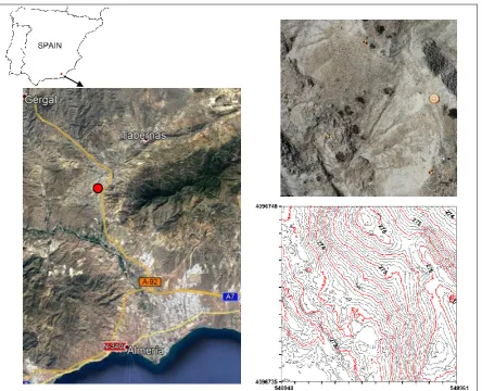
Figure 1. Location of the study area (red point in the figures of the left side), and orthophoto (right,
up) and contour map (right, down). Coordinates are UTM (zone 30, ETRS89).
2.2. Image collection
The images used in this work were taken from a rotatory wing DJI Mavic Air with four rotors. Its weight is 430 g, and it is equiped with a navigation system using GPS and GLONASS. In addition, it is equipped with a front, rear and lower vision system that allows it to detect surfaces with a defined pattern and adequate lighting, avoiding obstacles with a range between 0.5 and 10 m. Furthermore, the UAV is equipped with an RGB camera, mounted on a motion-compensated three-axis gimbal, with a 1/2.3” CMOS sensor, f/2.8 aperture, and 12 megapixels (4056 × 3040). The lens has a fixed focal length, equivlent to 35 mm format, of 24 mm and horizontal FOV of 85°.
The flight was carried out with an autopilot using the UgCS software [25], which allows to configure a flight altitude fitted parallel to the ground by a introducing a DSM of the study site. In this way, There is not scale difference between photographs. This DSM was generated previously in the same field visit through a photogrammetric project which was procesed on site. Flight altitude was set at a constant distance of 10 m, which yields a ground sample distance (GSD) of 0.46 cm. The forward and side overlaps were of 85% and 65%, respectively.
were ±9 and ±16 mm, respectively. Regardless, the purpose of this task was to get a high accuracy in the georeference of the DEM, not to check its accuracy.
2.3. Photogrammetric processing
The photogrammetric project was processed using Pix4Dmapper Pro version 3.1.23 [26], a software application based on the SfM and MVS techniques mentioned in the introduction section. The adjustments of this software were fitted in order to obtaind the highest 3D point cloud density. All the images were checked to avoid including blurred images in the project. Furthermore, the internal calibration parameters and coordinates of the image principal point of all the images were loaded from the EXIF data and considered as initial data for the iterative process of block adjustment. Identification of the GCPs in the images was carried out visually, using an incorporated tool in the processing software for assigning the absolute geolocation of the photogrammetric block. The product obtained from the photogrammetric project used in this study was the 3D point cloud.
2.4. 3D point cloud processing
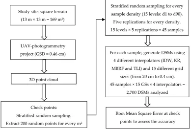
To study the influence of the 3D point cloud density, the interpolation method, and the GS of the derived DSM on the accuracy of that DSM, a factorial experimental design was carried out. Figure 2 shows the flowchart of the procedure followed in this study. The whole procedure described in this section was programmed using Golden Software ScripterTM, which allows to work with the Surfer 8.01 [27] modelization engine through instructions writen in a Visual Basic-like programming language.
Figure 2. Flowchart of the procedure followed in this study.
2.4.1. Data sets
Taking into account the objectives proposed in this work, the errors inherent in the coordinates of 3D points generated in the photogrammetric project have been considered null. From the initial 3D point cloud, a random sample of 200 Check Points (CPs) were extracted in every square meter of the study site. So, a total of 200 × 13 × 13 = 33,800 CPs were used for evaluating the derived DSM accuracy. Furthermore, after the CPs were extracted, 15 stratified random samples with different
Study site: square terrain
(13 m × 13 m = 169 m2)
Stratified random sampling for every
sample density (15 levels: d1 to d90).
Five replications for every density.
15 levels × 5 replications = 45 samples
UAV-photogrammetry
project (GSD = 0.46 cm)
3D point cloud
Check points:
Stratified random sampling.
Extract 200 random points for every m2
For each sample, generate DSMs using
4 different interpolators (IDW, KR,
MBRF and TLI) and 15 different grid
sizes (from 20 cm to 0.4 cm).
45 samples × 15 GSs × 4 interpolators =
2,700 DSMs analyzed
Root Mean Square Error at check
numbers of points were extracted, with five repetitions per sampling density. The sampling densities were those corresponding to 1, 2, 3, 4, 5, 10, 15, 20, 30, 40, 50, 60, 70, 80 and 90% of the total 3D points in the generated cloud, which are named as d1, d2, d3, d4, d5, d10, d15, d20, d30, d40, d5, d60, d70, d80, and d90, respectively. The raw point cloud is named as d100. These 5 × 15 = 45 files were extracted from the raw 3D point cloud using an informatics program developed by the authors in Visual Basic v6.0 language.
2.4.2. Interpolation methods
The interpolation methods evaluated in this work are Inverse Distance Weighted (IDW), Multiquadric Radial Basis Function (MRBF), Kriging (KR), and Triangulation with Linear Interpolation (TLI), which are all incorporated in the above-mentioned software Surfer 8.01. For each of the 45 extracted files and for each of the interpolation methods, the DSM grid size was set at 15 different values: 20, 15, 10, 9, 8, 7, 6, 5, 4, 3, 2, 1, 0.67, 0.5, and 0.4 cm. Then, 45 × 15 × 4 = 2,700 DSMs were analyzed.
Inverse Distance Weighted
This is a weighted average interpolator and one of the most used for surface modeling. It is based on the idea that the influence of one point relative to another declines with the distance from the grid node, where the value is interpolated. The weighting factor assigned to each data point fixes how this influence decreases when the distance increases. It is an exact and local interpolator which uses the next expression to estimate the value for a non-sampling point (x, y):
𝑍𝑗𝑒𝑠𝑡𝑖𝑚𝑎𝑡𝑒𝑑= ∑ 𝑍𝑖
𝑑𝑖𝑗𝛽 𝑖=𝑚𝑗 𝑖=1
∑ 1
𝑑𝑖𝑗𝛽 𝑖=𝑚𝑗 𝑖=1
, (1)
where 𝑍𝑗𝑒𝑠𝑡𝑖𝑚𝑎𝑡𝑒𝑑 is the interpolated height in the jth DSM node; Zi (I = 1, 2, …, mj) is the ith point
height of the cloud used to interpolate the jth DSM node; dij is the distance between the jth DSM node
and the ithpoint of the cloud used to interpolate the jth DSM node; mj is the number of points of the
cloud used to interpolate the jth DSM node; and β is the weighting power. In this study β= 2. Radial Basis Function
This exact interpolator includes a diverse group of interpolation methods which use a basic equation dependent on the distance between the interpolated point and the sampling points [28]. Its general expression generally used to interpolate topographic surfaces is:
𝑍𝑗𝑒𝑠𝑡𝑖𝑚𝑎𝑡𝑒𝑑= ∑ 𝑎 𝑖Ψ(𝑟𝑖𝑗) 𝑖=𝑚𝑗
𝑖=1 , (2)
where 𝑍𝑗𝑒𝑠𝑡𝑖𝑚𝑎𝑡𝑒𝑑 is the interpolated height in the jth DSM node; Ψ(𝑟𝑖𝑗) represents the radial basis functions; rij is the distance between the jth DSM node and the ith point of the cloud used to
interpolate the jth DSM node; ai are scalar values, called weights, associated to each point of the cloud
used to interpolate the jth DSM node; and mjis the number of points of the cloud used to interpolate
the jthDSM node.
To calculate the scalar values ai, it is necessary to solve the linear system M·A = Z, where M is an
mj-order square matrix containing the distances between the DSM node and the points used to interpolate thisnode, A is a vector containing the ai values which have to be calculated, and Z is a
vector containing the height of each point used to interpolate this node.
In terms of the ability to fit the data and to produce a smooth surface, the Multiquadric method is considered by many authors the best of all of the radial basis function methods [29,30]. In the MRBF, the radial basis functions take this form:
where r is the distance from the node to the point of the cloud, and c is the smoothing factor. There is no universal method to calculate this factor, and several authors have proposed different formulas (i.e. [31]). In this study, the following formula is used [27]:
𝑐2= 𝐷 2
25 × 𝑛, (4)
where D is the length of diagonal of the data extent, and n is the number of data points. Kriging
This is a geostatistical interpolation method that has demostrated good behavior in many fields. It attempts to express trends suggested in a data sample (3D point cloud), which means, for example, that high points might be connected along a ridge rather than isolated by bull’s-eye type contours. The general expresion for Ordinary Kriging is as follows:
𝑍𝑗𝑒𝑠𝑡𝑖𝑚𝑎𝑡𝑒𝑑 = ∑ 𝜆𝑖𝑍𝑖 𝑖=𝑚𝑗
𝑖=1 , (5)
where 𝑍𝑗𝑒𝑠𝑡𝑖𝑚𝑎𝑡𝑒𝑑 is the interpolated height in the jthDSM node. Zi (i = 1, 2, …, mj) is the ithpoint
height of the cloud used to interpolate the jthDSM node. λiis the weight associated to each point of
the cloud used to interpolate the jth DSM node. These values should be set so that the estimator is unbiased (∑ 𝜆𝑖
𝑖=𝑚𝑗
𝑖=1 = 1) and the variance is minimal. mj is the number of points of the cloud used to interpolate the jth DSM node.
Triangulation with Linear Interpolation
This is an exact interpolator which uses the optimal Delaunay triangulation [32] creating triangles by drawing lines between data points in such a way that no triangle edges are intersected by other triangles. In this way, the entire studied surface will be covered by a 3D triangle net, and the height estimation at a given grid node is made by linear interpolation taking into account the triangle which covers that node.
2.4.3. Evaluation of the DEM accuracy
As mentioned in Section 2.4.1, 33,800 points were extracted from the raw 3D point cloud to check the accuracy of the extracted elevations from the DSMs created from reduced point data densities. The measure to evaluate the performance of DSMs was the Root Mean Square Error (RMSE) [33]:
𝑅𝑀𝑆𝐸 = √∑ (𝑍𝑖
𝑒𝑠𝑡𝑖𝑚𝑎𝑡𝑒𝑑− 𝑍 𝑖𝑟𝑒𝑎𝑙)2 𝑖=𝑛
𝑖=1
𝑛 , (6)
where 𝑍𝑖𝑟𝑒𝑎𝑙 is the elevation of the ith (i = 1, 2, 3, …, 33,800) CP extracted from 3D point cloud, 𝑧𝑖𝑒𝑠𝑡𝑖𝑚𝑎𝑡𝑒𝑑 is the elevation estimated for the ith CP in the DSM under study, and n is the number of CPs (33800). A set of five RMSE values, corresponding to each replication, was calculated for each combination of 3D point cloud density, DSM grid size and interpolator. Analysis of variance (ANOVA) of the factorial model designed was carried out taking the RMSE as variable dependent, and the interpolation method and sampling density as the variation sources.
3. Results
Table 1. Correspondence between the studied percentages of points extracted from the raw point cloud, the number of points, the number of points per square meter, and the square grid size of a DSM that has as many nodes as points extracted from the raw cloud (equivalent square grid size).
Percentage 1 2 3 4 5 10 15 20
Number of points 105164 210329 315493 420658 525822 1051645 1577467 2103289
Points × m−2 622 1245 1867 2489 3111 6223 9334 12445
Equivalent square grid size (cm) 4.01 2.84 2.31 2.00 1.79 1.27 1.04 0.90
Percentage 30 40 50 60 70 80 90 100
Number of points 3154934 4206579 5258224 6309868 7361513 8413158 9464802 10516447
Points × m−2 18668 24891 31114 37336 43559 49782 56005 62227
Equivalent square grid size (cm) 0.73 0.63 0.57 0.52 0.48 0.45 0.42 0.40
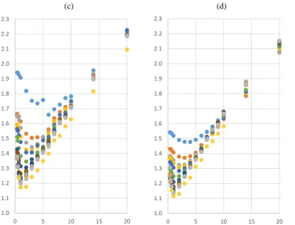
Figure 3 shows the relationship between the DSM grid size and the RMSE (average of five repetitions) for each point cloud density studied. As can be observed in this figure, all curves show a similar shape: as the GS decreases, the RMSE also decreases until a certain GS value, which is not the same in all cases but is close to 1 cm, from which the RMSE increases. Moreover, for the four interpolation methods, the curves are ordered to density, meaning that for a given interpolator, the curve corresponding to a certain density is below that corresponding to a lower density. For a given interpolation method, the differences in RMSE between different densities are lower at the extremes and higher in the central zone, which is precisely, as has just been said, where the minimum RMSE values are found. This means that the influence of point density on the RMSE for large and small GS values is not as noticeable as when the GS values are close to or somewhat greater than the optimum.
(a)
(b)
1.0 1.1 1.2 1.3 1.4 1.5 1.6 1.7 1.8 1.9 2.0 2.1 2.2 2.3
0 5 10 15 20
1.0 1.1 1.2 1.3 1.4 1.5 1.6 1.7 1.8 1.9 2.0 2.1 2.2 2.3
(c)
(d)
Figure 3. RMSE (y-axes, cm) for each GS (x-axes, cm), interpolation method and point cloud density.
Interpolation method: (a) IDW; (b) KR; (c) MRBF; (d) TLI. Point cloud density: ● d1; ● d2; ● d3; ● d4;
● d5; ● d10; ● d15; ● d20; ●d30; ● d40; ● d50; ●d60; ● d70; ● d80; ● d90; ● d100.
Table 2 shows the minimum RMSE (average of the five replications) and the GS for which it was reached, for every interpolator and 3D point cloud density studied. In this table, for a given RMSE column, values with the same letter are not statistically different (p < 0.05). In view of this table, it can be stated that for all interpolation methods, the minimum values of RMSE corresponding to a density equal to or greater than d20 have been reached for a GS equal to 1 cm. In view of this table, it can be stated that for all interpolation methods, the minimum RMSE values corresponding to a density equal to or greater than d20 have been reached for a GS equal to 1 cm. For densities lower than d20, the optimum GS varied depending on the interpolation method considered. In any case, up to d2, the highest optimum GS was 3 cm. For the lowest point density studied, d1, the optimal GS values are different for each interpolation method: 10, 4, 6, 3 cm for IDW, KR, MRBF, and TLI, respectively. The ANOVA and least significant difference tests carried out show that, considering each interpolation method separately, the RMSE values are grouped into statistically different sets (p < 0.05). These differences are most clearly shown for the IDW and KR methods, where there are no overlaps between the sets. For the MRBF and TLI, the value sets were not as well defined as for the other interpolators. RMSE values corresponding to d80 and d90 form a homogeneous group for all interpolation methods (MRBF and TLI have overlap with other groups of values).
1.0 1.1 1.2 1.3 1.4 1.5 1.6 1.7 1.8 1.9 2.0 2.1 2.2 2.3
0 5 10 15 20
1.0 1.1 1.2 1.3 1.4 1.5 1.6 1.7 1.8 1.9 2.0 2.1 2.2 2.3
Table 2. The minimum RMSE and the GS for which it was found, for every interpolator and 3D point cloud density studied. RMSE values are the average of the five replications. In each RMSE column, values with the same letter are not statistically different. The last row shows data corresponding to the raw 3D point cloud.
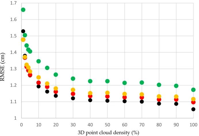
Figure 4 shows graphically the data presented in Table 2. Curves representing the minimum RMSE reached for every 3D point cloud density and every interpolation method show an asymptotic tendency, as the point density increases, toward the RMSE corresponding to d100. It can also be seen that the curve corresponding to the MRBF method is the one that is most separated from the rest.
IDW KR MRBF TLI
Density (%) GS RMSE Opt. GS RMSE GS RMSE GS RMSE
d1 10 1.529a 4 1.478a 6 1.660a 3 1.477a
d2 2 1.380b 3 1.368b 3 1.505b 3 1.372b
d3 2 1.318c 2 1.313c 3 1.442c 2 1.325c
d4 2 1.290d 2 1.291d 3 1.417c,d 2 1.309d
d5 2 1.260e 2 1.263e 3 1.406d 2 1.284e
d10 1 1.193f 2 1.216f 2 1.346e 1 1.248f
d15 1 1.162g 1 1.191g 2 1.306f 1 1.210g
d20 1 1.136h 1 1.161h 1 1.265g 1 1.181h
d30 1 1.121i 1 1.148i 1 1.241g,h 1 1.172h
d40 1 1.110j 1 1.135j 1 1.225h,i 1 1.152i
d50 1 1.106j 1 1.132j 1 1.225h,i 1 1.154i
d60 1 1.103j 1 1.127j 1 1.215h,i 1 1.148i
d70 1 1.101j 1 1.126j 1 1.217h,i 1 1.145i,j
d80 1 1.089k 1 1.114k 1 1.203i 1 1.133j
d90 1 1.088k 1 1.114k 1 1.197i 1 1.131j
3D point cloud density (%)
Figure 4.Minimum RMSE reached for every interpolator (● IDW; ● KR; ● MRBF; ● TLI) vs. 3D point
cloud density studied. RMSE values are the average of the five replications.
After the study of these results, two groups in every interpolation method were considered, one including RMSEs of d40 and other including d80. The ANOVA yields statistical differences (p < 0.05) between interpolation methods in both groups.
4. Discussion
UAV-derived 3D point clouds provide a new strategy for monitoring terrain surfaces with an extremely high level of spatial and temporal resolution. These clouds are used to derive DSMs, which provide a very useful basis to carry out calculus related to terrain monitoring. In the literature, virtually all work studying the accuracy of the DSMs generated from data acquired with SfM and MVS techniques does not separate the error due to the 3D point cloud generation process and the interpolation method used to generate the DSM, neither the fixed grid size nor the number of points in the point cloud.
All curves shown in Figure 3 (RMSE vs. GS, for all interpolation methods and densities studied), have a minimum RMSE value, reached for a certain GS, and values smaller than these yield worse RMSE, which indicates than the DSM generated does not fit as well as those generated with a bigger GS. Although there are works in which relations between the optimal grid size and other factors such as the point cloud density, terrain morphology, and others have been established (i.e. [34]), all of them being carried out for larger areas and point densities lower than those considered in this work, the results presented in this work do not show this relationship. Table 2 indicates that the GS for which the minimum RMSE has been reached for every interpolator and every density is not related to the 3D point cloud density and not related to the interpolation method. From d100 to d20, the optimum GS is 1 cm, and for values lower than d20 the optimum GSs adopt different values but they are not related to density and not related to the interpolator.
For all studied interpolation methods, data density was related to DSM accuracy: RMSE increased as data density decreased. This is because as the distance between the sample points increases, the accuracy of the DSM generated decreases [18]. Anderson et al. [18] studied a set of six reduced 3D point clouds derived from a series of 10 100-ha LiDAR-tiled study sites. Point densities ranged from 181.03 points × m−2 (no reduced point cloud) to 1.80 points × m−2 (1% of raw cloud). Furthermore, they used two interpolation methods: IDW and KR. For the IDW interpolator, the results showed an increase of RMSE from density equal to 100% (17.31 cm) to density equal to 1%
1 1.1 1.2 1.3 1.4 1.5 1.6 1.7
0 10 20 30 40 50 60 70 80 90 100
R
M
S
E
(
(35.66 cm). Then, the increase represented 106% of the minimum RMSE. For the KR interpolator, an increase from 001% (34.24 cm) to 1% (17.25 cm) represented 98.5% of the minimum RMSE. Liu et al. [19] found similar results using the IDW interpolator on a set of six reduced 3D point clouds derived from a raw LiDAR cloud. They studied densities from 0.037 points × m−2 (no reduced point cloud) to less than 0.001 points × m−2 (1% of raw cloud) in a study area of 113 km2. An increase of RMSE from 100% (18.4 cm) to 1% of 3D point cloud (64.1 cm) represented 248% with respect to the minimum RMSE. The study site of the present work is 169 m2 in area, and the point densities ranged (Table 1) from 62,227 points × m−2 (no reduced point cloud) to 622 points × m−2 (1% of raw cloud). This study, as opposed to those cited above, is looking for highly accurate and detailed microscale topography, and therefore the point densities should be higher than those used in the cited works. Taking into account the minimum and maximum RMSEs found for every interpolation method (Table 2), the increases represented 45% for IDW (from 1.529 to 1.054 cm), 35% for KR (from 1.478 to 1.097 cm), 42% for MRBF (from 1.660 to 1.173 cm), and 32% for TLI (from 1.477 to 1.116 cm). All these increases are lower than those reported by Anderson et al. [18] and Liu et al. [19]. Nevertheless, Asal [2] reported an increase of RMSE of approximately 260% when the point cloud was reduced to 6%.
For each density value studied, the RMSE values derived from the four interpolators were ordered from lowest to highest as follows: IDW, KR, TLI, and the worst values were found for RBF. Although differences between RMSEs derived from IDW, KR and TLI interpolators were not very high, the classical method IDW clearly proved to be more appropriate than the others, which agrees with some developers of UAV-photogrammetric software [26,35] that have incorporated this interpolation method to generate DSMs. Nevertheless, Anderson et al. [18] reported no RMSE discernible difference between IDW and KR. A similar conclusion was derived from their results by Lloyd and Atkinson [36].
Within each interpolation method, the least significant difference test carried out on RMSE yielded d80 and d90 as homogeneous groups (p < 0.05), another homogeneous group from d40 to d70, and densities from d30 to d1 are homogeneous groups themselves. All these homogeneous groups were clearly defined for IDW and KR. For TLI ,the groups were a bit more diffuse, and a bit more for RBF (Table 2). As with observed in data presented in this work, Anderson et al. [18], Liu et al. [19] and Asal [2] observed an asymptotic tendency of RMSE to d100 RMSE when point cloud density increases (Fig. 4), but they report a homogeneous RMSE group from d100 to d50, which does not agree with our results.
Elevation accuracy of DSM generated from UAV photogrammetry and SfM and MSV techniques reported in some works are 3.1 cm [37], 4 cm [38], 4.7 cm [39], or 6.62 cm [40], but none of them indicate the part of the error attributable to the DSM generation process, which could be desirable in order to define methodologies to maximize the accuracy of DSM.
5. Conclusions
UAV-photogrammetry based on SfM and MSV offers high-accuracy and high-density 3D point clouds for detailed representation of terrain surfaces. However, very high density data can entail redundant information and, therefore, large processing times to generate the DSM. Furthermore, knowledge of how each factor involved in the generation of DSM influences the error associated with it can help to develop methodologies to minimize this error.
This work studied how the 3D point cloud density and the interpolation method affect the DSM accuracy for data acquired from UAV and using SfM and MSV techniques.
The main conclusions derived from results exposed in this work are the following:
- Point cloud density, grid size and interpolation method significantly affect DSM accuracy. - Although differences of accuracy between IDW, KR, and TLI are not very high, IDW showed
the lower RMSE values. MRBF yielded the worse accuracies.
40% of the raw cloud, RMSE increases 5%. For densities lower than 15%, RMSE increases exponentially (45% for 1% of raw cloud).
- The grid size minimizing the RMSE for densities of 20% or higher was 1 cm, which represents 2 times the GSD of the pictures used for developing the photogrammetry project. Further analysis is needed to check generalizations of the conclusions: different surface morphologies, GSD, or even interpolation variant (power different than 2 in IDW interpolator, for example).
Author Contributions: The contributions of the authors were: conceptualization, F.A-V. and M.A-P.;
methodology, F.A-V. and M.A-P, F.C-R., and P.M-C.; software P.M.-C. and F.A.-V.; validation, F.M.; formal analysis, F.A-V., M.A-P., F.C-R. and P.M-C.; investigation, F.A-V and M.A-P; resources, P.M-C.; data curation, F.C.-R. and P.M.-C.; writing—original draft preparation, F.A-V and M.A-P.; writing—review and editing, F.A-V and M.A-P.; supervision, F.CR. and F.M.; project administration, F.A-F.A-V.; funding acquisition, F.A-F.A-V.
Funding: This research was funded by University of Almería (Spain), grant number CTM2017-88737-R,
“Proyectos Puente del Plan Propio de Investigación y Transferencia 2019”
Acknowledgments: Authors thanks to Peripheral Service of Research and Development based on drones,
University of Almería, Spain.
Conflicts of Interest: Authorsdeclarenoconflictofinterest. Thefundershadnoroleinthedesignofthestudy;in the
collection, analyses, or interpretation of data; in the writing of the manuscript, or in the decision to publish the results.
References
1. Mancini, F.; Dubbini, M.; Gattelli, M.; Stecchi, F.; Fabbri, S.; Gabbianelli, G. Using Unmanned Aerial Vehicles (UAV) for High-Resolution Reconstruction of Topography: The Structure
from Motion Approach on Coastal Environments. Remote Sens. 2013, 5, 6880–6898.
2. Asal, F.F. EVALUATING the EFFECTS of REDUCTIONS in LiDAR DATA on the VISUAL
and STATISTICAL CHARACTERISTICS of the CREATED DIGITAL ELEVATION MODELS. ISPRS Ann. Photogramm. Remote Sens. Spat. Inf. Sci. 2016, 3, 91–98.
3. Jaud, M.; Passot, S.; Le Bivic, R.; Delacourt, C.; Grandjean, P.; Le Dantec, N. Assessing the accuracy of high resolution digital surface models computed by PhotoScan® and MicMac®
in sub-optimal survey conditions. Remote Sens. 2016, 8.
4. Agüera-Vega, F.; Carvajal-Ramírez, F.; Martínez-Carricondo, P.; Sánchez-Hermosilla López,
J.; Mesas-Carrascosa, F.J.; García-Ferrer, A.; Pérez-Porras, F.J. Reconstruction of extreme topography from UAV structure from motion photogrammetry. Meas. J. Int. Meas. Confed. 2018, 121, 127–138.
5. Martinez-Guanter, J.; Agüera, P.; Agüera, J.; Pérez-Ruiz, M. Spray and economics assessment of a UAV-based ultra-low-volume application in olive and citrus orchards. Precis. Agric. 2019. 6. Campos, J.; Llop, J.; Gallart, M.; García-Ruiz, F.; Gras, A.; Salcedo, R.; Gil, E. Development of canopy vigour maps using UAV for site-specific management during vineyard spraying
process. Precis. Agric. 2019.
7. Agüera Vega, F.; Ramírez, F.C.; Saiz, M.P.; Rosúa, F.O. Multi-temporal imaging using an
unmanned aerial vehicle for monitoring a sunflower crop. Biosyst. Eng. 2015, 132.
8. Rossi, G.; Tanteri, L.; Tofani, V.; Vannocci, P.; Moretti, S.; Casagli, N. Multitemporal UAV
surveys for landslide mapping and characterization. Landslides 2018, 15, 1045–1052.
9. Gong, C.; Lei, S.; Bian, Z.; Liu, Y.; Zhang, Z.; Cheng, W. Analysis of the Development of an
Low-Cost UAVs. Remote Sens. 2019, 11, 1356.
10. Atkinson, K.B. Close Range Photogrammetry and Machine Vision; Whitttles, 1996; ISBN 187032546X.
11. Richard Hartley, A.Z. Multiple View Geometry; 2003; Vol. 53; ISBN 9788578110796.
12. Snavely, N.; Seitz, S.M.; Szeliski, R. Modeling the World from Internet Photo Collections. Int. J. Comput. Vis. 2008, 80, 189–210.
13. Westoby, M.J.; Brasington, J.; Glasser, N.F.; Hambrey, M.J.; Reynolds, J.M. ?Structure-from-Motion? photogrammetry: A low-cost, effective tool for geoscience applications.
Geomorphology 2012, 179, 300–314.
14. Vasuki, Y.; Holden, E.-J.; Kovesi, P.; Micklethwaite, S. Semi-automatic mapping of geological
Structures using UAV-based photogrammetric data: An image analysis approach. Comput. Geosci. 2014, 69, 22–32.
15. Remondino, F.; El-Hakim, S. Image-based 3D Modelling: A Review. Photogramm. Rec. 2006, 21, 269–291.
16. Juan, L.; Gwun, O. A comparison of sift, pca-sift and surf. Int. J. Image Process. 2009, 3, 143–
152.
17. Singh, K.K.; Chen, G.; McCarter, J.B.; Meentemeyer, R.K. Effects of LiDAR point density and
landscape context on estimates of urban forest biomass. ISPRS J. Photogramm. Remote Sens. 2015, 101, 310–322.
18. Anderson, E.S.; Thompson, J.A.; Austin, R.E. LIDAR density and linear interpolator effects on elevation estimates. Int. J. Remote Sens. 2005, 26, 3889–3900.
19. Liu, X.; Zhang, Z.; Peterson, J.; Chandra, S. The effect of LiDAR data density on DEM accuracy. Int. Congr. Model. Simul. 2007, 1363–1369.
20. Liu, X.; Zhang, Z. Lidar Data Reduction for Efficient and High Quality Dem Generation. Int. Arch. Photogramm. Remote Sens. Spat. Inf. Sci. 2008, XXXVII, 173–178.
21. Asensio, C.; Weber, J.; Lozano, F.; Mielnik, L. Laser-scanner used in a wind tunnel to quantify
soil erosion. Int. Agrophysics 2019, 33, 227–232.
22. Schmid, T.; Schack-Kirchner, H.; Hildebrand, E. A case study of terrestrial laser scanning in
erosion research: calculation of roughness and volume balance at a logged forest site. Int. Arch. Photogramm. Remote Sens. Spat. Inf. Sci. 2014, XXXVI-8/, 114–118.
23. García-Serrana, M.; Gulliver, J.S.; Nieber, J.L. Description of soil micro-topography and fractional wetted area under runoff using fractal dimensions. Earth Surf. Process. Landforms 2018, 43, 2685–2697.
24. Smith, M.W.; Warburton, J. Microtopography of bare peat: a conceptual model and objective classification from high-resolution topographic survey data; 2018; Vol. 43; ISBN 0000000343619. 25. UgCS https://www.ugcs.com/.
26. Pix4Dmapper No
Titlehttps://www.pix4d.com/product/pix4dmapper-photogrammetry-software.
27. Golden Software https://www.goldensoftware.com/products/surfer.
28. Carlson, R.E.; Foley, T.A. Interpolation of track data with radial basis methods. Comput. Math. with Appl. 1992, 24, 27–34.
29. Franke, R. Scattered Data Interpolation: Test of Some Methods. Math. Comput. 1982, 33, 181–
200.
C.D. of A.M. and T., Ed.; 1990; Vol. 12, pp. 105–209.
31. Carlson, R.E.; Foley, T.A. The parameter R2 in multiquadric interpolation. Comput. Math. with Appl. 1991, 21, 29–42.
32. Lee, D.T.; Schachter, B.J. Two algorithms for constructing a Delaunay triangulation. Int. J. Comput. Inf. Sci. 1980, 9, 219–242.
33. Yang, X.; Hodler, T. Visual and Statistical Comparisons of Surface Modeling Techniques for Point-based Environmental Data. Cartogr. Geogr. Inf. Sci. 2000, 27, 165–176.
34. Hengl, T. Finding the right pixel size. Comput. Geosci. 2006, 32, 1283–1298. 35. Agisoft Metashape No Titlehttps://www.agisoft.com/.
36. Lloyd, C.D.; Atkinson, P.M. Deriving DSMs from LiDAR data with kriging. Int. J. Remote Sens. 2002, 23, 2519–2524.
37. Cryderman, C.; Bill Mah, S.; Shufletoski, A. Evaluation of UAV Photogrammetric Accuracy
for Mapping and Earthworks Computations. GEOMATICA 2014, 68, 309–317.
38. Oniga, V.-E.; Breaban, A.-I.; Statescu, F. Determining the Optimum Number of Ground
Control Points for Obtaining High Precision Results Based on UAS Images. Proceedings 2018, 2.
39. Agüera-Vega, F.; Carvajal-Ramírez, F.; Martínez-Carricondo, P. Accuracy of digital surface
models and orthophotos derived from unmanned aerial vehicle photogrammetry. J. Surv. Eng. 2017, 143.