PASSIVE NEAR-FIELD SOURCE LOCALIZATION BASED ON SPATIAL-TEMPORAL STRUCTURE
Y. Wu
Wuhan Institute of Technology Wuhan 430073, China
H. C. So
Department of Electronic Engineering City University of Hong Kong
Kowloon, Hong Kong, China
C. Hou
Institute of Acoustics
Chinese Academy of Sciences Beijing 100080, China
Abstract—A new subspace method based on spatial-temporal
structure is presented for estimation of directions-of-arrival (DOA’s) and ranges of multiple near-field sources impinging on an array of sensors. The arrival angle and range parameters are directly given by the eigenvalues of a set of constructed matrices and the computational complexity of the proposed method is lower than those of several available methods which do not require search operation. Simulation results show that the proposed method outperforms an ESPRIT-like method.
1. INTRODUCTION
In array signal processing, many methods for estimation of direction-of-arrival (DOA) of far-field source impinging on an array of sensors have been developed [1], such as MUSIC and ESPRIT. Most of these methods assume that the received sources are located relatively far from the array and hence the wavefronts from the sources can be
regarded as plane waves. With this assumption, each source location can be characterized by a single DOA [1]. When the source is close to the array which corresponds to the near-field scenario, the plane wave assumption is no longer valid. The near-field sources must be characterized by spherical wavefronts at the array aperture and need to be localized by both range and DOA [2–5]. Note that the near-field situation is common in applications for sonar [2], seismic exploration [3] and electronic surveillance [8], etc.
accuracy.
In this paper, a spatial-temporal structure based method for joint DOA and range estimation of near-field sources is presented. The motivation for using the spatial-temporal structure of spatial correlation sequences is to reduce the effect of observed noise as well as to achieve performance improvement in the case of limited data snapshots by constructing the so-called “pseudo-snapshots” [14, 15]. The proposed method uses only second-order statistics and is suitable for both Gaussian and non-Gaussian signal sources. A closed-form estimation of both DOA and range is provided through a subspace method. The rest of the paper is organized as follows. Section 2 describes the data model for the near-field source localization and the problem formulation. The proposed algorithm is developed in Section 3. Finally, simulation results are provided in Section 4, followed by a conclusion in Section 5.
2. PROBLEM FORMULATION
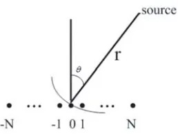
We consider the narrow-band model for array processing of near-field sources where there areP narrow-band sources received by a uniform linear array of n= 2N + 1 sensors with inter-element spacingd. The array configuration is shown in Figure 1. For unique estimation, we require d ≤ λ/4 [10] where λ denotes the wavelength of the source wavefronts and N > P. The output of the mth sensor can be approximated as [2–11]:
xm(t) =
P
i=1
si(t)ej(ωim+φim2)+
nm(t), t= 1,2, . . . , M (1)
for m =−N, . . . ,0,1, . . . , N. It is assumed that P is known a priori and the P sources {s1(t), . . . , sP(t)} are statistically independent of each other while the additive noise component nm(t) is a zero-mean white Gaussian process and is independent of the source signals. Here we let the sensor m = 0 be the phase reference point, which is also the origin of our coordinate system. The parameters ωi and φi are
functions of the azimuth angle θi and rangeri of the ith source, and
they are expressed as
ωi = −2π
λ dsin(θi) and φi = d2π
λri cos
2(
Figure 1. Configuration of uniform linear array.
3. THE PROPOSED ALGORITHM
The proposed method can be divided into two steps and uses only second-order statistics of the array output. The first step is a signal pre-processing which consists of the computation of some properly chosen spatial correlation sequences of the observed signal. These correlation coefficients are shown to be superimposed exponential sequences and their frequencies are linear functions of angles and ranges of the source signals.
The second step is to transform the cross-correlated spatial sequences of the observed signal from 1-D space domain to 2-D space-time domain and then use a subspace rotation invariance technique to obtain the estimates of ωi and φi.
Under the assumption of spatial-temporal white Gaussian noise, the correlation sequences for{xm(t)} are:
r(−l,l)(τ) =
P
i=1
rsisi(τ)e−2jωil+σ2δ(l+τ) (3)
r(−l−1,l)(τ) =
P
i=1
rsisi(τ)e−j(ωi−φi)(2l+1) (4)
r(−l+1,l)(τ) =
P
i=1
rsisi(τ)e−j(ωi+φi)(2l−1) (5)
where
r(k,l)(τ) =E{xk(t+τ /2)xl∗(t−τ /2)}, k=−N, . . . ,0, l= 0,1, . . . , N (6) and
is the autocorrelation function of ith source where ∗ denotes the conjugate operator, σ2 is the noise power of nm(t) and δ(·) is the
impulse function. It is noteworthy that we will ignore the noise term in (3) atl= 0 andτ = 0 in the following development asσ2 is assumed known a priori or accurately estimated [16].
Equations (3)–(5) show that the noise-free correlation sequence corresponds to the time series of harmonic sequences with harmonic frequencies given by ωi, ωi−φi and ωi+φi, respectively. Therefore,
we can estimate the harmonic components by a subspace-based high-resolution estimation method.
Forl= 0,1,2, . . . , N, we define the following vectors with the use of (3)–(5):
X(τ) = [r(0,0)(τ), r(−1,1)(τ), . . . , r(−N,N)(τ)]T(N+1)×1 (8)
Y(τ) = [r(−1,0)(τ), r(−2,1)(τ), . . . , r(−N,N−1)(τ)]TN×1 (9)
Z(τ) = [r(1,0)(τ), r(0,1)(τ), . . . , r(−N+1,N)(τ)]T(N+1)×1 (10) where T denotes the transpose operator. Note that the dimension of
Y(τ) is different from those ofX(τ) andZ(τ). We can rewrite (8)–(10) in matrix form as:
X(τ) = Ax(ω1, ω2, . . . , ωP)Rs(τ) (11) Y(τ) = Ay(ω1−φ1, ω2−φ2, . . . , ωP −φP)Rs(τ) (12) Z(τ) = Az(ω1+φ1, ω2+φ2, . . . , ωP +φP)Rs(τ) (13)
where
Rs(τ) = [rs1s1(τ), . . . , rsisi(τ), . . . , rsPsP(τ)]T (14)
Ax =
⎛ ⎜ ⎜ ⎝
1 . . . 1 e−j2ω1 . . . e−j2ωP
..
. ... ... e−j2ω1N . . . e−j2ωPN
⎞ ⎟ ⎟ ⎠
(N+1)×P
(15)
Ay =
⎛ ⎜ ⎜ ⎜ ⎝
e−j(ω1−φ1) . . . e−j(ωP−φP) e−j3(ω1−φ1) . . . e−j3(ωP−φP)
..
. ... ...
e−j(2N+1)(ω1−φ1) . . . e−j(2N+1)(ωP−φP)
⎞ ⎟ ⎟ ⎟ ⎠
N×P
(16)
Az =
⎛ ⎜ ⎜ ⎜ ⎝
e−j(−1)(ω1+φ1) . . . e−j(−1)(ωP+φP) e−j(ω1+φ1) . . . e−j(ωP+φP)
..
. ... ...
e−j(2N−1)(ω1+φ1) . . . e−j(2N−1)(ωP+φP)
⎞ ⎟ ⎟ ⎟ ⎠
We sample again the correlation sequences
{r(−l,l)(τ), r(−l−1,l)(τ), r(−l+1,l)(τ)}
atK lags whereK denotes the number of “pseudo-snapshots” [14, 15]. Let τ = 0, Ts,2Ts, . . . ,(K − 1)Ts where Ts represents the sample
interval of the pseudo-snapshots which is chosen as an integral multiple of the original sample interval of the observed dataxm(t). As a result,
(K−1)Tsis always smaller than the number of samples of the observed
array data M. The value of K should satisfy N < (K−1) ≤M/Ts
and (K−1)Ts ≤Lis required to ensurersisi((K−1)Ts)= 0 whereL
is the correlation length of the source signals.
We then obtain the following data matrices using the spatial-temporal samples,
Rx= [X(0Ts),X(Ts),X(2Ts), . . . ,X((K−1)Ts)](N+1)×K=AxR0(18)
Ry= [Y(0Ts),Y(Ts),Y(2Ts), . . . ,Y((K−1)Ts)]N×K=AyR0 (19)
Rz= [Z(0Ts),Z(Ts),Z(2Ts), . . . ,Z((K−1)Ts)](N+1)×K=AzR0 (20) where
R0 = [Rs(0),Rs(Ts), . . . ,Rs((K−1)Ts)]P×K (21) Now we define
Rx1 =Rx(1 :N,:) and Rx2 =Rx(2 : (N + 1),:) (22) whereRx(k:l,:) takes thek-th to l-th rows of Rx. We have
Rx1 =Ax1Rs and Rx2 =Ax1ΦxRs (23)
where
Ax1=Ax(1 :N,:) (24)
and
Φx =
⎛ ⎜ ⎜ ⎝
e−j2ω1 0 . . . 0 0 e−j2ω2 . . . 0
..
. ... . .. ... 0 0 . . . e−j2ωP
⎞ ⎟ ⎟
⎠ (25)
It is assumed that the matrices Ax and R0 are of full rank. The full rank assumption of Ax is classical and is generally valid for real applications. In applications such as radar, sonar and wireless communications, the a priori knowledge of source signals is available and hence the condition that R0 is full rank can be satisfied [14, 15]. Following [15], we can easily obtain:
whereR1 is calculated as
R1=Rx2[Rx1]# (27)
with (·)# denotes the pseudo-inverse of a matrix. Similar to (21)–(23), we use (19)–(20) to obtain:
R2Ay1 =Ay1Φy and R3Az1 =Az1Φz (28)
where
R2 = Ry(2 :N,:)[Ry(1 : (N −1),:)]# (29)
R3 = Rz(2 : (N + 1),:)[Rz(1 :N,:)]# (30)
Ay1 = Ay(1 : (N−1),:) and Az1=Az(1 :N,:) (31)
Φy =
⎛ ⎜ ⎜ ⎜ ⎝
e−j2(ω1−φ1) 0 . . . 0 0 e−j2(ω2−φ2) . . . 0 ..
. ... . .. ...
0 0 . . . e−j2(ωP−φP)
⎞ ⎟ ⎟ ⎟
⎠ (32)
and
Φz=
⎛ ⎜ ⎜ ⎜ ⎝
e−j2(ω1+φ1) 0 . . . 0 0 e−j2(ω2+φ2) . . . 0
..
. ... . .. ...
0 0 . . . e−j2(ωP+φP)
⎞ ⎟ ⎟ ⎟
⎠ (33)
Note that the dimensions ofR1,R2 and R3 areN×N,(N−1)×(N1) and N ×N, respectively. As a result, the estimates of the matrices
Φx, Φy, and Φz can be given by the P nonzero eigenvalues from the eigenvalue decomposition ofR1,R2, andR3, respectively. The angles and ranges estimates are easily computed by the diagonal elements of
Φx,Φy, and Φz.
To estimate the ranges and angles of the sources, we first need to pair the elements of the three sets of parameters, namely, {ωˆi}, {ωˆi −φˆi}, and {ωˆi + ˆφi} where ˆωi and ˆφi represent the estimate of
ωi and φi, respectively. This is achieved as follows [11]. For each ˆωi,
1≤i≤P, its corresponding value of ˆφi is obtained as: ˆ
φi = ωˆl0 + ˆφl0
−ωˆk0 −φˆk0
/2 (34) where the indexes (k0, l0) are given by
(k0, l0) = arg min
k,l
ωˆi− ωˆk+ ˆφk
+
ˆ ωl−φˆl
From each pair of (ˆωi,φˆi), i = 1,2, . . . , P, the estimates of the DOA
and range parameters, denoted by ˆθiand ˆri, respectively, are computed
as
ˆ
θi= sin−1
−λωˆi
2πd
(36)
ˆ ri= πd
2cos2θˆ
i
λφiˆ (37)
The procedure of the proposed algorithm is summarized as
• Compute the estimates ofr(−l,l)(τ), r(−l−1,l)(τ) andr(−l+1,l)(τ) in (3)–(5) with removing the noise term in (3), and then construct
X(τ), Y(τ), Z(τ) using (8)–(10).
• ConstructRx, Ry, Rz according to (18)–(20).
• ComputeR1,R2 and R3 using (27), (29) and (30).
• Perform eigenvalue decomposition ofRi, i= 1,2,3, to obtain the corresponding eigenvalues, and then the parameter estimates, ˆωi,
ˆ
ωi−φˆiand ˆωi+ ˆφi, are calculated with the use of the phase angles of the corresponding eigenvalues.
• Pair the estimated parameters{ωˆi,ωˆi−φˆi,ωˆi+ ˆφi}using (34) and
(35) and then get (ˆωi,φˆi).
• Compute the source location parameters, ˆθiand ˆri,i= 1,2, . . . , P,
using (36) and (37).
4. SIMULATION RESULTS
A set of computer simulations is carried out to evaluate the performance of the proposed method. We consider a uniform linear array ofn= 2N+ 1 sensors with inter-element spacing ofd=λ/4. All the sensor noise components {nm(t)} are zero-mean white Gaussian
processes with identical powers. Both Gaussian and non-Gaussian signal sources are investigated. The performance is measured by the root mean square error (RMSE).
In the first experiment, there are n = 7 sensors or N = 3. Two non-Gaussian signal sources with equal powers, which are of the forms of s1(t) = ej(0.2πt+ϕ1) and s2(t) = ej(0.4πt+ϕ2) where {ϕi} are independent and are uniformly distributed in [0,2π], are impinging on this array. The first source is located at θ1 = 40◦ with a range of r1 = 5λ, and the second is located at θ2 = 20◦ with r2 = 1.5λ. The number of samples is set to M = 20 and the number of pseudo-snapshots isK = 10 with Ts= 2. All results provided are averages of
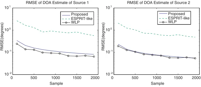
100 independent runs. The RMSEs for the DOA and range estimates of the two sources are shown in Figures 2 and 3. For comparison, the results using the ESPRIT-like algorithm [10] as well as the WLP method [12] are also shown. We can see that the estimation accuracy of the proposed method is comparable to that of the WLP method, but it is much higher than that of ESPRIT-like method over all signal-to-noise ratio (SNR) conditions. Note that the performance of DOA estimation is similar for both sources while the RMSE of the range estimate for s2(t) is much lower than that of s1(t) because the second source is close to the array while the first source is far from it, and this agrees with the findings in [13].
-10 -5 0 5 10 15 20 25 30 10-4
10-3
10-2
10-1
100
101
SNR(dB)
RMSE(degrees)
RMSE of DOA Estimate of Source 1
Proposed ESPRIT-like WLP
-10 -5 0 5 10 15 20 25 30 10-3
10-2 10-1 100 101
SNR(dB)
RMSE(degrees)
RMSE of DOA Estimate of Source 2
Proposed ESPRIT-like WLP
-10 -5 0 5 10 15 20 25 30 10-3
10-2
10-1
100
101
SNR(dB)
RMSE(wavelengths)
RMSE of Range Estimate of Source 1
Proposed ESPRIT-like WLP
-10 -5 0 5 10 15 20 25 30 10-4
10-3
10-2
10-1
100
101
SNR(dB)
RMSE(wavelengths)
RMSE of Range Estimate of Source 2
Proposed ESPRIT-like WLP
Figure 3. RMSEs of estimated ranges versus input SNR.
0 500 1000 1500 2000
10-2
10-1
100
101
Sample
RMSE(degrees)
RMSE of DOA Estimate of Source 1
Proposed ESPRIT-like WLP
0 500 1000 1500 2000
10-2
10-1
100
101
Sample
RMSE(degrees)
RMSE of DOA Estimate of Source 2
Proposed ESPRIT-like WLP
Figure 4. RMSEs of estimated DOA’s versusM.
In the third experiment, we consider two equal-power non-Gaussian signals impinging on an array of 9 sensors with SNR = 20 dB, M = 50 and K = 25. The first source position is characterized by (40◦,1.5λ) while the DOA of the second source is fixed at 20◦ with its range varies from 5λto 20λ. 100 independent runs are conducted for each range parameter and the results for the DOA estimates are shown in Figure 5. We see that the performance of the proposed and WLP methods is much better than that of ESPRIT-like method for different ranges of the second source.
5 10 15 20
10-3
10-2
10-1
Range of Source 2 (wavelengths)
RMSE(degrees)
RMSE of DOA Estimate of Source 1
Proposed ESPRIT-like WLP
5 10 15 20
10-3
10-2
10-1
Range of Source 2 (wavelengths)
RMSE(degrees)
RMSE of DOA Estimate of Source 2
Proposed ESPRIT-like WLP
Figure 5. RMSEs of estimated DOA’s versus range of second source.
0 50
-5 0 5 10 15 20
Angle(degrees)
Range(wavelengths)
Proposed method
0 50
-5 0 5 10 15 20
Angle(degrees)
Range(wavelengths)
ESPRIT like method
0 50
-5 0 5 10 15 20
Angle(degrees)
Range(wavelengths)
WLP method
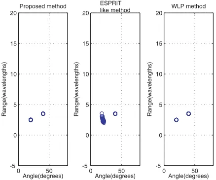
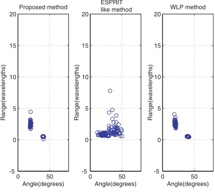
In the fourth experiment, the positions of the first and second non-Gaussian sources are characterized by (40◦,3.5λ) and (20◦,2.5λ), respectively, and they have different input SNR values, namely, 20 dB and 10 dB. We assign n= 11, M = 50 and K= 25. The results based on 50 independent runs are shown in Figure 6. We observe that the proposed and WLS methods are comparable and their performance is better than that of the ESPRIT-like method when the two sources have unequal noise powers.
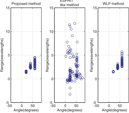
In the fifth experiment, we consider that there are three non-Gaussian uncorrelated signal sources impinging on the received array. The first and second source signals are same as before while s3(t) = ej(0.8πt+ϕ3), and the position parameters are (60◦,3.5λ), (40◦,2.5λ), (20◦,1.5λ), respectively. The input SNRs of all received signals are equal to 20 dB while n = 15, M = 100 and K = 50. It is shown in Figure 7 that the performance of the proposed method and the WLS scheme is comparable and they are superior to the ESPRIT-like method, particularly for the range estimates [13].
In the last experiment, we consider two uncorrelated colored Gaussian signal sources whose positions are parameterized by (40◦,0.5λ) and (20◦,2.5λ). The input SNRs of the two signals are both equal to 20 dB while n= 11, M = 100 andK = 50. The results based on 50 independent runs are shown in Figure 8. As mentioned
-50 0 50 -5
0 5 10 15
Angle(degrees)
Range(wavelengths)
Proposed method
-50 0 50 -5
0 5 10 15
Angle(degrees)
Range(wavelengths)
ESPRIT like method
-50 0 50 -5
0 5 10 15
Angle(degrees)
Range(wavelengths)
WLP method
Figure 7. Estimated ranges and DOA’s for three non-Gaussian
in Section 1, the ESPRIT-like method which utilizes the fourth-order cumulants fails to resolve the two Gaussian signal sources. On the other hand, it is seen that the two methods using second-order statistics can still give accurate estimates of ranges and angles for colored Gaussian signal sources.
0 50
-5 0 5 10 15 20
Angle(degrees)
Range(wavelengths)
Proposed method
0 50
-5 0 5 10 15 20
Angle(degrees)
Range(wavelengths)
ESPRIT like method
0 50
-5 0 5 10 15 20
Angle(degrees)
Range(wavelengths)
WLP method
Figure 8. Estimated ranges and DOA’s for two Gaussian signal
sources with equal powers.
5. CONCLUSION
ACKNOWLEDGMENT
This work described in this paper was jointly supported by a grant from the National Natural Science Foundation of China (Project No. 60802046) and the Research Plan Project of Hubei Provincial Department of Education (No. Q20091501).
REFERENCES
1. Krim, H. and M. Viberg, “Two decades of array signal processing research: The parametric approach,” IEEE Signal Processing Magazine, Vol. 13, No. 4, 67–94, July 1996.
2. Kim, J. H., I. S. Yang, K. M. Kim, and W. T. Oh, “Passive ranging sonar based on multi-beam towed array,” Proc. IEEE Oceans, Vol. 3, 1495–1499, September 2000.
3. Swindlelhurst, A. L. and T. Kailath, “Passive direction of arrival and range estimation for near-field sources,”IEEE Spec. Est. and Mod. Workshop, 123–128, 1988.
4. Huang, Y. D. and M. Barkat, “Near-field multiple sources localization by passive sensor array,” IEEE Trans. Antennas Propag., Vol. 39, 968–975, July 1991.
5. Jeffers, R., K. L. Bell, and H. L. Van Trees, “Broadband passive range estimation using MUSIC,” Proc. IEEE Int. Conf. Acoust. Speech, Signal Processing, Vol. 3, 2920–2922, Orlando, Florida, USA, May 2002.
6. Starer, D. and A. Nehorai, “Path-following algorithm for passive localization of near-field sources,” 5th ASSP Workshop on Spectrum Estimation and Modeling, 322–326, October 1990. 7. Lee, J. H., C. M. Lee, and K. K. Lee, “A modified path-following
algorithm using a known algebraic path,” IEEE Trans. Signal Processing, Vol. 47, 1407–2409, May 1999.
8. Lee, C. M., K. S. Yoon, and K. K. Lee, “Efficient algorithm for localising 3-D narrowband multiple sources,” IEE Proc. Radar, Sonar Navig., Vol. 148, 23–26, Febuary 2001.
9. Weiss, A. J. and B. Friedlander, “Range and bearing estimation using polynomial rooting,” IEEE J. Ocean. Engr., Vol. 18, 130– 137, April 1993.
11. Grosicki, E. and K. Abed-Meraim, “A weighted linear prediction method for near-field source localization,” Proc. IEEE Int. Conf. Acoust. Speech, Signal Processing, 2957–2960, Orlando, Florida, USA, May 2002.
12. Grosicki, E., K. Abed-Meraim, and Y. Hua, “A weighted linear prediction method for near-field source localization,”IEEE Trans. Signal Process., Vol. 53, 3651–3660, October 2005.
13. Yuen, N. and B. Friedlander, “Performance analysis of higher-order ESPRIT for localization of near-field sources,”IEEE Trans. Signal Processing, Vol. 46, No. 3, 709–719, March 1998.
14. Jin, L., Q.-Y. Yin, and B.-F. Jiang, “Direction finding of wideband signals via spatial-temporal processing in wireless communications,” Prof. IEEE International Symposium on Circuits and Systems, Vol. 2, 81–84, Geneva, Switzerland, May 2000.
15. Deng, K., Q. Yin, L. Ding, and Z. Zhao, “Blind channel estimator for V-BLAST coded DS-CDMA system in frequency selective fading environment,”Proc. IEEE VTC’2003 Fall, Orlando, USA, 458–462, 2003.