One-loop perturbative coupling of A and A★ through the chiral overlap operator

One-loop perturbative coupling of

A

and

A

through the chiral

overlap operator

HirokiMakino1_{,OkutoMorikawa}1,_{, andHiroshiSuzuki}1,

1_{Department of Physics, Kyushu University 744 Motooka, Nishi-ku, Fukuoka, 819-0395, Japan}

Abstract.Recently, Grabowska and Kaplan constructed a four-dimensional lattice for-mulation of chiral gauge theories on the basis of the chiral overlap operator. At least in the tree-level approximation, the left-handed fermion is coupled only to the original gauge fieldA, while the right-handed one is coupled only to the gauge fieldA, a de-formation ofAby the gradient flow with infinite flow time. In this paper, we study the fermion one-loop effective action in their formulation. We show that the continuum limit

of this effective action contains local interaction terms betweenAand A, even if the anomaly cancellation condition is met. These non-vanishing terms would lead an unde-sired perturbative spectrum in the formulation.

1 Introduction and discussion

Recently, Grabowska and Kaplan proposed a four-dimensional lattice formulation of chiral gauge theories [1]. This formulation is based on the so-called overlap operator, which can be obtained from their five-dimensional domain-wall formulation [2]1_{by the traditional way [4–6]. In this formulation,}

along the fifth dimension, the original gauge fieldAis deformed by the gradient flow [7–10] for infinite flow time. Since the gradient flow preserves the gauge covariance, this formulation is manifestly gauge invariant,even if the anomaly cancellation condition is not met. Although there is a subtlety associated with the topological charge [1,2,11–13], the smeared gauge field after the infinite-flow time, A, only to which the right-handed (invisible) fermion would be coupled, can be basically considered as pure gauge (see AppendixA). Then one would regard their setup as the system of the left-handed fermion interacting with the gauge fieldA;2_{this picture was however confirmed only in}

the tree-level approximation [1]. It is thus a crucial problem whether radiative corrections induce the physical coupling of the right-handed fermion or not.

First, let us see the tree-level decoupling between the physical and invisible sectors. So far, only when the transition of the flowed gauge field along the fifth dimension is abrupt, the four-dimensional lattice Dirac operator has been obtained as an explicit form; this is referred to as the chiral overlap

_{Speaker, e-mail: [email protected]}

_{Acknowledges partial support by JSPS Grants-in-Aid for Scientific Research Grant Number JP16H03982.} 1_{As a closely related six-dimensional domain-wall formulation, see Ref. [3].}

operator ˆDχ. The operator ˆDχis given by [1]

aDˆχ=1+γ5

1−(1−) 1 +1

(1−)

, (1)

whereais the lattice spacing, and() is the sign function [15,16]

≡ Hw(A) Hw(A)2

 

≡

Hw(A)

Hw(A)2  

, (2)

of the Hermitian Wilson Dirac operator

Hw=γ5 ₁

2γµ(∇µ+∇∗µ)− 1

2a∇µ∇∗µ−m

, (3)

wheremis the parameter of the domain-wall height, andγµis the Dirac matrix. In this expression,∇µ is the forward gauge covariant lattice derivative and∇∗

µis the backward one. With the assumption of abruptness, this Dirac operator depends on the two gauge fields,AandA. In the classical continuum limit [1],

amDˆχ

a→0

→ γµDµ(A)P−+γµDµ(A)P+, (4)

whereDµ(A) (Dµ(A)) is the covariant derivative defined with respect toA(A), andP±=(1±γ5)/2

are the chirality projection operators. Therefore, the coupling between the gauge fields,AandA, is not produced in the tree-level approximation.

Let us study how the decoupling betweenAandAis modified under radiative corrections. The fermion one-loop effective action is defined by

lnZ[A,A]≡ln x

_{dψ(x)dψ¯(x)exp} −a4

x ¯

ψ(x) ˆDχψ(x)  

, (5)

whereAandAare regarded as independent non-dynamical variables. To investigate the (de)coupling, two infinitesimal variationsδandδare introduced such thatδacts only onAbut not onA,

δA0, δA≡0, (6)

andδacts in an opposite way,

δA≡0, δA0. (7)

Then, we will find that in the continuum limit a double variation of the effective action is given as

δδlnZ[A,A]=−

d4_{xL(A,A;δA, δA), (8)}

whereL(A,A;δA, δA) is alocalpolynomial of its arguments and their spacetime derivatives. To find a possible implication of Eq. (8), we takegauge variationsasδandδ:

δωAµ(x)≡∂µω(x)+[Aµ(x), ω(x)], δωAµ(x)=0, (9) δωAµ(x)≡∂µω(x)+[Aµ(x), ω(x)], δωAµ(x)=0. (10)

Since, as a property of the gradient flow, the two gauge fieldsAandAtransform in the same way under the gauge transformation, the gauge invariance of the effective action implies

(δω_+δω

operator ˆDχ. The operator ˆDχis given by [1]

aDˆχ=1+γ5

1−(1−) 1 +1

(1−)

, (1)

whereais the lattice spacing, and() is the sign function [15,16]

≡ Hw(A) Hw(A)2

 

≡

Hw(A)

Hw(A)2  

, (2)

of the Hermitian Wilson Dirac operator

Hw=γ5 ₁

2γµ(∇µ+∇∗µ)− 1

2a∇µ∇∗µ−m

, (3)

wheremis the parameter of the domain-wall height, andγµis the Dirac matrix. In this expression,∇µ is the forward gauge covariant lattice derivative and∇∗

µis the backward one. With the assumption of abruptness, this Dirac operator depends on the two gauge fields,AandA. In the classical continuum limit [1],

amDˆχ

a→0

→ γµDµ(A)P−+γµDµ(A)P+, (4)

whereDµ(A) (Dµ(A)) is the covariant derivative defined with respect toA(A), andP±=(1±γ5)/2

are the chirality projection operators. Therefore, the coupling between the gauge fields,AandA, is not produced in the tree-level approximation.

Let us study how the decoupling betweenAandAis modified under radiative corrections. The fermion one-loop effective action is defined by

lnZ[A,A]≡ln x

_{dψ(x)dψ¯(x)exp} −a4

x ¯

ψ(x) ˆDχψ(x)  

, (5)

whereAandAare regarded as independent non-dynamical variables. To investigate the (de)coupling, two infinitesimal variationsδandδare introduced such thatδacts only onAbut not onA,

δA0, δA≡0, (6)

andδacts in an opposite way,

δA≡0, δA0. (7)

Then, we will find that in the continuum limit a double variation of the effective action is given as

δδlnZ[A,A]=−

d4_{xL(A,A;δA, δA), (8)}

whereL(A,A;δA, δA) is alocalpolynomial of its arguments and their spacetime derivatives. To find a possible implication of Eq. (8), we takegauge variationsasδandδ:

δωAµ(x)≡∂µω(x)+[Aµ(x), ω(x)], δωAµ(x)=0, (9) δωAµ(x)≡∂µω(x)+[Aµ(x), ω(x)], δωAµ(x)=0. (10)

Since, as a property of the gradient flow, the two gauge fieldsAandA transform in the same way under the gauge transformation, the gauge invariance of the effective action implies

(δω_+δω

) lnZ[A,A]=0⇒δ(δω+δω) lnZ[A,A]=0. (11)

Therefore, using Eq. (8), we can obtain

δδωZ[A,A]=−δδωZ[A,A]=

d4xL(A,A;δA, δωA). (12)

Now, let us assume thatAbecomes pure gauge under the gradient flow with infinite flow time (see AppendixA):

A=g−1dg. (13)

Then the gauge transformationAg−1

makesA=0, where

Ag_=g−1_{(d+A)g. (14)}

That is, we can impose theA=0 gauge on Eq. (12)

δδωlnZ[A,0]=

d4_{xL(A,A=0;δA, δ}ω

A|A=0). (15)

We will see below that the right-hand side does not vanish even if the anomaly cancellation condition is met.

It will be shown in the next section that lnZ[A,0] has the term

lnZ[A,0]=

d4_x f0

2a2trAµAµ+· · ·, (16)

thus the mass term trAµAµis produced in the one-loop level. The propagator of the gauge potential in thisA=0 thus has the structure,

Aa

µ(x)Aaν(y)

=g2₀δab

_d4p

(2π)4eip(x−y)

δµν− pµpν

p2

₁

p2_+m2

A+· · ·

, (17)

where we have defined the mass parametermAas

m2

A=g20 f0

2a2. (18)

Therefore, the perturbative spectrum is modified in aweird way; this would not be what we want to obtain for chiral gauge theories. Since these effects in the one-loop effective action (16) should be removed by local counterterms, the formulation of Grabowska and Kaplan will be undesirable as a non-perturbative formulation of chiral gauge theories. Then their formulation with the abrupt transition should be improved in some possible way.

2 Explicit forms of

_L

and

δ

ω

_ln

_Z

In this section, we show the results of the continuum limit ofL(A,A;δA, δA).3 In what follows, we use the variables

Cµ≡Aµ−Aµ, (19)

¯

Aµ≡1₂(Aµ+Aµ), (20)

¯

Dµ≡∂µ+[ ¯Aµ,·], (21)

and the field strength

¯

Fµν =∂µAν¯ −∂νAµ¯ +[ ¯Aµ,Aν¯ ]. (22)

We also define the following lattice integrals:

f0(am)≡

p

  −₄1_t−

s2 ρ 4t−

ccρ 4t

 

, (23)

f1(am)≡

p

  ₆₄1_t2 −

cρcσ 128t +

s2 ρs2σ 32t2  

, (24)

f2(am)≡

p

 

−cρcσ_32t + 7s2

ρs2σ 64t2 +

cs2 ρcσ 32t2 +

c2_cρcσ

64t2  

, (25)

f3(am)≡

p

 

−cρcσ_32t +3s

2 ρs2σ 32t2 −

s2 ρ 32t2 −

ccρ 32t2

 

, (26)

f4(am)≡

p

  ₉₆1_t+

s2 ρ 96t+

ccρ 96t+

1 16t2

 

, (27)

f5(am)≡

p

 

₁₆1_t+cρcσ_32t +₃₂7_t2 − c2

32t2 + ccρ 16t2 +

s2 ρ 32t2

 

, (28)

where

sρ≡sinpρ, cρ ≡cospρ, (29)

c≡

µ

(cµ−1)+am, t≡

µ s2

µ+c2, (30)

p≡

π

−π d4_p

(2π)4. (31)

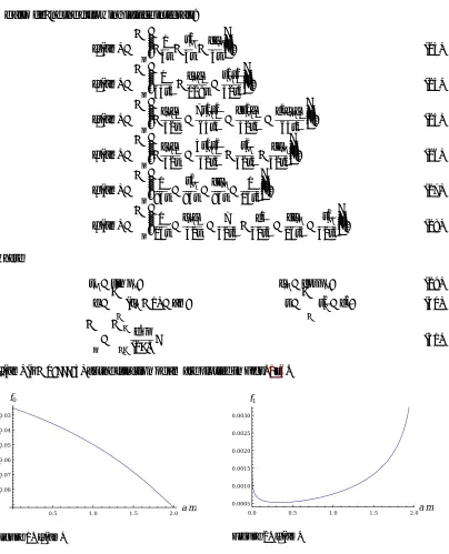
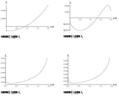
fi(am) (i=0, . . . ,5) as the function ofamare plotted in Figs.1–6.

0.5 1.0 1.5 2.0a m

0.08

0.07

0.06

0.05

0.04

0.03

f0

Figure 1. f0(am)

0.0 0.5 1.0 1.5 2.0a m 0.0005

0.0010 0.0015 0.0020 0.0025 0.0030

f1

Figure 2. f1(am)

and the field strength

¯

Fµν =∂µAν¯ −∂νAµ¯ +[ ¯Aµ,Aν¯ ]. (22)

We also define the following lattice integrals:

f0(am)≡

p

  −₄1_t−

s2 ρ 4t −

ccρ 4t

 

, (23)

f1(am)≡

p

  ₆₄1_t2 −

cρcσ 128t +

s2 ρs2σ 32t2  

, (24)

f2(am)≡

p

 

−cρcσ_32t + 7s2

ρs2σ 64t2 +

cs2_ρcσ

32t2 + c2_cρcσ

64t2  

, (25)

f3(am)≡

p

 

−cρcσ_32t +3s

2 ρs2σ 32t2 −

s2 ρ 32t2 −

ccρ 32t2

 

, (26)

f4(am)≡

p

  ₉₆1_t+

s2 ρ 96t+

ccρ 96t+

1 16t2

 

, (27)

f5(am)≡

p

 

₁₆1_t+cρcσ_32t +₃₂7_t2 − c2

32t2 + ccρ 16t2 +

s2 ρ 32t2

 

, (28)

where

sρ ≡sinpρ, cρ≡cospρ, (29)

c≡

µ

(cµ−1)+am, t≡

µ s2

µ+c2, (30)

p ≡

π

−π d4_p

(2π)4. (31)

fi(am) (i=0, . . . ,5) as the function ofamare plotted in Figs.1–6.

0.5 1.0 1.5 2.0a m

0.08 0.07 0.06 0.05 0.04 0.03 f0

Figure 1. f0(am)

0.0 0.5 1.0 1.5 2.0a m 0.0005 0.0010 0.0015 0.0020 0.0025 0.0030 f1

Figure 2. f1(am)

The local functional Lhas three parts, according to the parity and Lorentz symmetry: (i) the parity-odd and Lorentz-preserving part, (ii) the parity-even and Lorentz-preserving part, and (iii) the

0.5 1.0 1.5 2.0a m 0.0005

0.0010

f2

Figure 3. f2(am)

0.5 1.0 1.5 2.0a m

0.0002

0.0001 0.0001 0.0002

f3

Figure 4. f3(am)

0.0 0.5 1.0 1.5 2.0a m

0.004 0.006 0.008 0.010 0.012 0.014 f4

Figure 5. f4(am)

0.0 0.5 1.0 1.5 2.0a m

0.010 0.015 0.020 0.025 0.030 0.035 0.040 0.045 f5

Figure 6. f5(am)

parity-even and Lorentz-violating part. First, the parity-odd part ofLis given by

L(A,A;δA, δA)|parity-odd

=− 1 32π2µνρσ

¯ Fµν+ 1

12[Cµ,Cν]

{δAρ, δAσ}

−1₃Cµ{δAν,Dρ¯ δAσ}+{δAν,Dρ¯ δAσ}

, (32)

we have the parity-even and Lorentz-preserving part ofL,

L(A,A;δA, δA)|parity-even, Lorentz-preserving

= f0

a2δAµδAµ

+

−3₂f1 + f2 2 −

f3

2

[( ¯DµδAµ)CνδAν−CµδAµ( ¯DνδAν)]

−

_f 1

2 + f2

2 − 3f3

2

[Cµ( ¯DνδAµ)δAν−δAµCν( ¯DµδAν)]

−

_f 1

2 + f2

2 − 3f3

2

[CνδAµ( ¯DµδAν)−( ¯DνδAµ)CµδAν]

+

−7₂f1 + f2 2 +

f3

2

[( ¯DµCµ)δAνδAν−δAν( ¯DµCµ)δAν]

−

_3f 1

2 − f2

2 + f3

2

[δAµCµ( ¯DνδAν)−Cν( ¯DµδAµ)δAν]

+(13f₁−3f₂−3f₃) ( ¯DµδAµ)( ¯DνδAν)

+(9f₁₋3f₂₋f₃) ( ¯DµδAν)( ¯DµδAν)

+(−19f1+5f2+5f3) ( ¯DνδAµ)( ¯DµδAν)

+ _11f

1

6 −

f2

6 − 7f3

6

CµδAνCµδAν

+

−13₆f1 +11f2

6 −

7f3

6

(CµδAµCνδAν+CνδAµCµδAν)

+

−5₁₂f1 +19f2 12 −

17f3

12

(CνCµδAµδAν+δAµCµCνδAν)

+

19f1

12 − 5f2

12 − 5f3

12

(CµCνδAµδAν+δAµCνCµδAν)

+

−17₁₂f1 +19f2 12 −

11f3

12

(CµCµδAνδAν+δAνCµCµδAν), (33)

and finally the parity-even and Lorentz-violating part is given by

L(A,A;δA, δA)|_{parity-even, Lorentz-violating}

=3 2

9f1−f2− f3− f₂4 − f₂5

[( ¯DνCν)δAνδAν−δAν( ¯DνCν)δAν]

−

9f1−f2−f3− f₂4 − f₂5

( ¯DνδAν)( ¯DνδAν)

+

47f1

2 −

7f2

2 − 7f3

2 + f4

4 − 7f5

4

CνδAνCνδAν

+ _67f

1

4 −

11f2

4 −

11f3

4 +

5f4

8 − 11f5

8

(CνCνδAνδAν+δAνCνCνδAν). (34)

we have the parity-even and Lorentz-preserving part ofL,

L(A,A;δA, δA)|parity-even, Lorentz-preserving

= f0

a2δAµδAµ

+

−3₂f1 + f2 2 −

f3

2

[( ¯DµδAµ)CνδAν−CµδAµ( ¯DνδAν)]

− _f 1 2 + f2 2 − 3f3

2

[Cµ( ¯DνδAµ)δAν−δAµCν( ¯DµδAν)]

− _f 1 2 + f2 2 − 3f3

2

[CνδAµ( ¯DµδAν)−( ¯DνδAµ)CµδAν]

+

−7₂f1 + f2 2 +

f3

2

[( ¯DµCµ)δAνδAν−δAν( ¯DµCµ)δAν]

− _3f 1 2 − f2 2 + f3 2

[δAµCµ( ¯DνδAν)−Cν( ¯DµδAµ)δAν]

+(13f₁−3f₂−3f₃) ( ¯DµδAµ)( ¯DνδAν)

+(9f₁₋3f₂₋f₃) ( ¯DµδAν)( ¯DµδAν)

+(−19f1+5f2+5f3) ( ¯DνδAµ)( ¯DµδAν)

+ _11f 1 6 − f2 6 − 7f3

6

CµδAνCµδAν

+

−13₆f1 +11f2

6 −

7f3

6

(CµδAµCνδAν+CνδAµCµδAν)

+

−5₁₂f1 +19f2 12 −

17f3

12

(CνCµδAµδAν+δAµCµCνδAν)

+

19f1

12 − 5f2

12 − 5f3

12

(CµCνδAµδAν+δAµCνCµδAν)

+

−17₁₂f1 +19f2 12 −

11f3

12

(CµCµδAνδAν+δAνCµCµδAν), (33)

and finally the parity-even and Lorentz-violating part is given by

L(A,A;δA, δA)|parity-even, Lorentz-violating

= 3 2

9f1−f2−f3− f₂4 − f₂5

[( ¯DνCν)δAνδAν−δAν( ¯DνCν)δAν]

−

9f1−f2−f3− f₂4 − f₂5

( ¯DνδAν)( ¯DνδAν)

+

47f1

2 −

7f2

2 − 7f3

2 + f4

4 − 7f5

4

CνδAνCνδAν

+ _67f

1

4 −

11f2

4 −

11f3

4 +

5f4

8 − 11f5

8

(CνCνδAνδAν+δAνCνCνδAν). (34)

By using the above form ofL(A,A;δA, δA), one can deduce the gauge variation of lnZ[A,0], δω_{lnZ[A,0] (see Appendix A of Ref. [17] for details). The parity-odd part ofLgives rise to (leaving}

out the symbol d4_xtr)

δωlnZ[A,0]|parity-odd=₂₄1_π2µνρσ(∂µω)

Aν∂ρAσ+1 2AνAρAσ

, (35)

which is the consistent gauge anomaly associated with a left-handed fermion. It is impossible to rewrite this expression as the gauge variation of a local term. On the other hand, the parity-even part ofδω_{lnZcan be written as the gauge variation of local terms:}

δωlnZ[A,0]|parity-even

=δω

f0

2a2AµAµ

+1

2(−13f1+3f2+3f3)Aµ∂µ∂νAν

+(5f₁₋f₂₋2f₃)(Aµ∂ν∂νAµ−AµAν∂µAν+AµAν∂νAµ)

+2

3(f1+f2−2f3)AµAµAνAν+ 1

12(−11f1+f2+7f3)AµAνAµAν

+1 2

9f1−f2−f3− f₂4 − f₂5

Aµ∂µ∂µAµ

+1 4

19f1−3f2−3f3+ f₂4 −3₂f5

AµAµAµAµ

. (36)

The last two lines are not Lorentz invariant. This parity-even part does not vanish even if the gauge representation is anomaly-free. For example, the first termδω_[(f

0/2a2)AµAµ] corresponds to the gauge

variation of the mass term of the gauge field. Theregularization garbagein Eq. (36) can be subtracted by local counterterms. However, such a necessity for counterterms will be undesirable from a per-spective of a non-perturbative formulation of chiral gauge theories.

We would like to thank Shoji Hashimoto, Yoshio Kikukawa, and Ken-ichi Okumura for valuable remarks. We are grateful to Ryuichiro Kitano and Katsumasa Nakayama for intensive discussions on a related subject.

A Gradient flow for infinite flow time

The gradient flow of the gauge field is defined by

∂tBµ(t,x)=DνGνµ(t,x), Bµ(t=0,x)=Aµ(x). (37)

In the abelian theory, we can solve this equation as

Bµ(t,x)=

d4_y d4p

(2π)4e

ip(x−y)_δ µν−

pµpν p2

e−tp2

+ pµpν

p2

Aν(y). (38)

This shows that after infinite flow time the configuration becomes pure gauge:

Bµ(t,x)t→∞→ g(x)−1∂µg(x), (39)

where

g(x)=exp

−

d4_y d4p

(2π)4 eip(x−y)

p2 ∂µAµ(y)

Note thatg(x) is a non-local functional of the original gauge fieldAµ(y).

For the non-abelian theory, we cannot solve the flow equation in a closed form. However, we can show that the Euclidean action integralS = d4x₄1_g2

0G

a

µν(x)Gaµν(x) monotonically decreases along the flow. Since the minimum of the action integral in the topologically trivial sector is given by a pure gauge configuration, the flowed configuration in the topologically trivial sector approaches a pure gauge configuration. In fact, the pure gauge configuration

Bµ(t,x)=g(x)−1∂µg(x) (41)

is a stationary solution of the flow equation,∂tB(t,x)=0.

References

[1] D. M. Grabowska and D. B. Kaplan, Phys. Rev. D94no.11, 114504 (2016) [arXiv:1610.02151 [hep-lat]].

[2] D. M. Grabowska and D. B. Kaplan, Phys. Rev. Lett. 116 no.21, 211602 (2016) [arXiv:1511.03649 [hep-lat]].

[3] H. Fukaya, T. Onogi, S. Yamamoto and R. Yamamura, PTEP 2017 no.3, 033B06 (2017) [arXiv:1607.06174 [hep-th]].

[4] H. Neuberger, Phys. Rev. D57, 5417 (1998) [hep-lat/9710089]. [5] P. M. Vranas, Phys. Rev. D57, 1415 (1998) [hep-lat/9705023].

[6] Y. Kikukawa and T. Noguchi,Lattice field theory. Proceedings, 17th International Symposium, Lattice’99, Pisa, Italy, June 29-July 3, 1999, Nucl. Phys. Proc. Suppl. 83 (2000) 630 [hep-lat/9902022].

[7] R. Narayanan and H. Neuberger, JHEP0603, 064 (2006) [hep-th/0601210]. [8] M. Lüscher, Commun. Math. Phys.293, 899 (2010) [arXiv:0907.5491 [hep-lat]].

[9] M. Lüscher, JHEP1008, 071 (2010) Erratum: [JHEP1403, 092 (2014)] [arXiv:1006.4518 [hep-lat]].

[10] M. Lüscher and P. Weisz, JHEP1102, 051 (2011) [arXiv:1101.0963 [hep-th]].

[11] K. Okumura and H. Suzuki, PTEP2016no.12, 123B07 (2016) [arXiv:1608.02217 [hep-lat]]. [12] H. Makino and O. Morikawa, PTEP2016no.12, 123B06 (2016) [arXiv:1609.08376 [hep-lat]]. [13] Y. Hamada and H. Kawai, PTEP2017no.6, 063B09 (2017) [arXiv:1705.01317 [hep-lat]]. [14] L. Álvarez-Gaumé and P. H. Ginsparg, Nucl. Phys. B243, 449 (1984).

[15] H. Neuberger, Phys. Lett. B417, 141 (1998) [hep-lat/9707022]. [16] H. Neuberger, Phys. Lett. B427, 353 (1998) [hep-lat/9801031].