Article
1
A helical charge simulation based 3-D method for
2
calculating AC stranded conductor’s corona loss in
3
the corona cage
4
Yunpeng Liu1, Shilong Huang1*, Shugang Liu1, Daran Liu 1, and Zhicheng Huang1
5
1 Hebei Provincial Key Laboratory of Power Transmission Equipment Security Defense, North China Electric
6
Power University, No.619 North of Yonghua Street, Baoding 071003, China; [email protected](Y.L.);
7
[email protected](S.L.); [email protected](D.L.); [email protected](Z.H.)
8
* Correspondence: [email protected]; Tel.: +86-151-0020-8295
9
10
11
Abstract: Corona loss generated from conductors is one of the important design factors on ac
12
transmission lines. Based on helical charge simulation method, the 3-D calculation model for
13
corona loss considering the conductors’ outer strands in the corona cage is established. With regard
14
to 2-D corona-loss calculation method, the calculation model proposed in this paper can take the
15
electric field strength’s nonuniformity along the axial direction of stranded conductor into
16
consideration, furthermore, it can also calculate the corona loss when the conductor has sag. The
17
calculation results of the LGJ-300/40 and LGJ-400/35 in the small corona cage well coincide with the
18
measurement results, which indicate that the corona-loss calculation model is appropriate. In
19
addition, the corona loss of the bundle conductors 4 × LGJ720 with sag in UHV corona cage is also
20
analyzed.
21
Keywords: corona loss, helical charge, 3-D calculation model, stranded conductor, sag
22
23
1. Introduction
24
In alternating current (AC) lines, when the field strength around transmission line exceeds the
25
breakdown electric field strength of air, the air near the conductor is ionized, which is called corona
26
discharge. The corona discharge results in the production of different space charge (positive ions,
27
negative ions and electrons), the charge carriers showing different polarity with the conductor are
28
attracted to the conductor and may lose their charge on the conductor surface while those with
29
similar polarity with the conductor are pushed away from it towards the ground. The energy loss
30
caused by such back-and-forth movement of space charge in power cycle is called corona loss.
31
Corona loss, which has been researched for many years, shows important significances for
32
conductors selection, and is a considerable criterion for measuring the operation economy of
33
transmission lines [1-4].
34
Up to now, AC conductors’ corona loss has been extensively studied through experiments
35
using small indoor corona cage, large outdoor corona cage and test lines. The test results show that
36
these factors including conductor radius, bundle number, bundle spacing, distance to ground and
37
surface roughness coefficients can influence corona loss [5-12].
38
When AC voltage is applied, the space line charge will go back and forth at power frequency,
39
and it’s more difficult to calculate ac ion-flow field, therefore, there is little research on the
40
calculation model of AC conductors’ corona loss. Clade, Abdel-Salam, Li, Liu researched the
41
calculation model. Clade calculated the corona loss of single conductor in corona cage based on
42
Kaptzov and Deutch assumptions while ignoring the influences of space charges on the electric
43
field direction[13-15]. By abandoning the Deutsch assumption, Abdel-Salam researched the single,
44
triple and multi phases transmission-line corona loss, but he did not consider the inhomogeneity of
45
electric field on the conductor surface and believed that charges on the conductor surface are emitted
46
uniformly [16,17]. By taking charge emission’s inhomogeneity on the conductors surface into
47
consideration, Li researched the ion flow of multiphase and bundle conductors [18]. Liu adopted
48
the Li’s improved calculation model and researched the corona loss of single and bundle conductors
49
in the corona cage [19,20].
50
However, the present corona loss calculation models are all for 2-D models, which assume that
51
the conductor has infinite length as well as smooth and straight structure, ingoring the electric-field
52
strength’s nonuniformity along the axial direction of stranded conductor. Due to the finite length
53
and conductors’ external twisting structure, the electric field strength on the conductor surface were
54
uneven. Meanwhile, the 2-D calculation model can’t take the conductor’s sag or wind lean into
55
consideration either. so it is necessary to develop a 3-D calculation model for corona loss .
56
In this paper, simulation charges which have the same spiral form as the outer strand of the
57
conductor are used to calculate corona loss of the conductor owing to spirally wounded outer
58
strand of the conductor [21]. Every corona cage wall is equivalent to the ground plane and
59
simulated by the helical charge as well. By utilizing the Kaptzov assumption and abandoning the
60
Deutsch assumption, the processes including emission, transfer and recombination of space line
61
charges are simulated considering the inhomogeneity of charge emission on the surface of
62
conductor, and the 3-D calculation model for corona loss in the corona cage is established. The
63
calculation model’s accuracy is verified through test data in small corona cage and UHV corona
64
cage.
65
2. Calculation methods
66
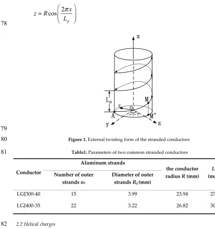
2.1. Twisting form of the external of stranded conductors
67
The conductors’ outer strand is spirally winded on inner strand. If a point M(x,y,z) in a space
68
rotates about x axis at the angular velocity ωon a cylindrical surface y2+z2=R2 ,and rises along the
69
positive direction parallel to x axis at the linear velocity ʋ, the motion track of point M is known as a
70
helical line. When ωt=2π, the distance h of point M moving along the axial direction is called the
71
pitch. As shown in Figure 1, the pitch length Lp = PF×2R in engineering, PF is the conductor’s pitch
72
factor and R is outer diameter. Parameters of two common conductors are shown in Table 1 [23].
73
Hence, the location of point M which is related to the Lp and the conductor radius R can be obtained
74
through (1)–(3).
75
2
π
θ
=
L
px
(1)
76
2
sin
π
=
p
x
y R
L
(2)
2
cos
π
=
p
x
z R
L
(3)
78
79
Figure 1. External twisting form of the stranded conductors
80
Table1. Parameters of two common stranded conductors
81
Conductor
Aluminum strands
the conductor radiusR (mm)
Lp
(mm) PF
Number of outer strands n0
Diameter of outer strands Rg (mm)
LGJ300-40
LGJ400-35
15
22
3.99
3.22
23.94
26.82
277
300
10-12
10-12
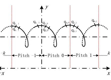
2.2 Helical charges
82
The simulation helical charges are placed inside each strand of the external layer and take the
83
same helical shape as the strand and repeat along x-axis after a pitch, assuming that conductor is
84
finite long and segmented into finite number of pitches (-k…,-1,0,1,…+k), in each pitch, any helical
85
charge, qh, is divided into n finite line charges, having length l and equal projections along the x-axis,
86
as demonstrated in Figure 2. The number of simulation helical charges qh is assumed to be 3 times
87
the number of strands in the outer layer (3 ×no), ngsimulationhelical charges are placed on corona
88
cage walls, that is, the total number of simulation line charges with an equal pitch is N=n×(3×
89
n0+ng). Owing to simulation line charges are repetitions of equal pitch along x direction, the
90
unknown simulation line charges are only those in Pitch0, and the rest simulation line charges can be
91
obtained through the coordinate transformation.
93
Figure2. Helical charges
94
95
96
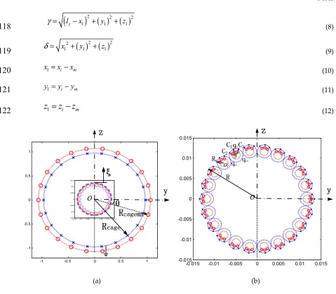
Coordinates of simulation line charges and boundary points.
97
Figure 3 illustrates the cross section of LGJ400-35 which has n0=22, an overall radius
98
R=13.41mm in the corona cage. Where, the red ‘o’ and blue ‘×’ represent the arrangement points of
99
simulation helical charges and boundary points, respectively. Inside each strand of the outer layer,
100
the three helical simulation charge qh1, qh2and qh3 are assumed to be spaced radially from the strand center
101
with the distances of f1Rg, f2Rg and f3Rg, where, Rg is the strand radius, 0<f2=f3<f1<1. Ψindicates the
102
deviation angle of helical charges qh2 and qh3 to qh1. When a corona cage with a square section is
103
equivalent to a cylindrical one, the equivalent diameter Rcage =1.08×L, L is the cross-section dimension
104
of the corona cage [4]. In order to verify whether the potential boundary conditions are met, the
105
boundary points with the same number and deviation angle are chosen on the outer strands and
106
corona cage surface corresponding to the each simulation line charge, hence, N boundary points are
107
chosen for Pitch0, and each boundary point lies on its locus at the middle of the corresponding
108
simulation line charge. The sketch map of helical charges with Pitch0 is shown in Figure 4.
109
Due to the simulation linear charges with charge Qj (Qj= qj,0, j = 1, 2, . . . , N), supposing that the
110
starting coordinate is Am(xm,ym,zm) and the length is lj, the potential coefficient Pi,j and field strength
111
coefficients fxij, fyij and fzij at arbitrary point Ai(xi,yi,zi) are shown as follows:
112
(
)
( )
1 0 1 1 ln 4 γ πε δ − + = − + j ij j l x P l x (4)113
01 1 1
4πε γ δ
= − ij j fx l (5)
114
( ) ( )
(
)
1 1 1 2 20 1 1
1
4πε γ δ
− = + + j ij j l x y x fy
l y z
(6)
115
( ) ( )
(
)
1 1 1 2 20 1 1
1
4πε γ δ
− = + + j ij j l x z x fz
l y z
(7)
116
Where,
(
)
2( ) ( )
2 21 1 1
γ
= lj−x + y + z(8)
118
( ) ( )
2 2 21 1 1
δ
= x + y + z(9)
119
1= −i m
x x x (10)
120
1= −i m
y y y (11)
121
1
= −
i mz
z
z
(12)
122
(a) (b)
Figure 4.The location of helical charges and boundary points in the cross section.(a) Arrangement of
123
simulation helical charges and boundary on the corona cage and conductor; (b) Arrangement of
124
simulation helical charges and boundary on the conductor.
125
-1 -0.5 0 0.5 1
-1 -0.5 0 0.5 1
-0.015 -0.01 -0.005 0 0.005 0.01 0.015 -0.015
-0.01 -0.005 0 0.005 0.01 0.015
-0.015 -0.01 -0.005 0 0.005 0.01 0.015 -0.015
(a)
(b)
Figure4. Helical charges’ arrangement of with Pitch0 on the conductor (a) Main view of helical
126
charges’ arrangement (b) Top view of helical charges arrangement
127
2.3. Corona onset and charge emission
128
According to the Kaptzov assumption, the corona onset charge at different points on the
129
conductor surface is calculated by considering the influences of space charge. Supposing that
130
voltage Ut = Uapp·sin(ω·t)is applied at moment t, then,
131
+ + =
cond cond space space cage cage t
P Q P Q P Q U
(13)
132
1 + 1 + 1 =0
cond cond space space cage cage
P Q P Q P Q
(14)
133
1cos cosδ β 1sinβ 1sin cosδ β
= + +
x x y z
E E E E
(15)
134
1cos sinδ β 1cosβ 1sin sinδ β
= + +
y x y z
E E E E
(16)
135
1sin
δ
1cosδ
= +
z x z
E E E (17)
136
Where,
137
1= + +
x cond cond space space cage cage
E fx Q fx Q fx Q
(18)
138
1= + +
y cond cond space space cage cage
E fy Q fy Q fy Q
(19)
139
1= + +
z cond cond space space cage cage
E fz Q fz Q fz Q
(20)
140
In (13), (14), (18) and (19), Qcond, Qspace and Qcage represent the vector of simulation line charges of
141
the conductor, space and cage walls, respectively.
142
-0.015 -0.01
-0.005 0
0.005 0.01
0.015
-0.02 -0.01 0 0.01 0.02
0 0.05 0.1 0.15 0.2 0.25 0.3 0.35
-0.015 -0.01 -0.005 0 0.005 0.01 0.015 -0.015
In (13), Pcond, Pspace and Pcage are the potential coefficient matrix of Qcond, Qspace and Qcage to the charge
143
emitting points on the surface of the conductor, respectively.
144
In (14), Pcond1, Pspace1 and Pcage1 are the potential coefficient matrix of Qcond, Qspace and Qcage to the
145
boundary points on corona cage wall, respectively.
146
Equating the applied voltage with calculated potential at boundary points, the unknown
147
simulation charges can be determined through (13) and (14).
148
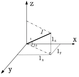
In (15)-(17), δandβare the inclination angles vector of line charges having length l on the x-y
149
and x-z planes, as demonstrated in Figure 5.
150
151
Figure 5.theinclination angles of linear charges on thex-y and x-z planes
152
In (18), fxcond, fxspace and fxcage are the field strength coefficients matrix of Qcond, Qspace and Qcage to the
153
emitting points on the conductor surface at the x direction, respectively.
154
In (19), fycond, fyspace and fycage are the field strength coefficients matrix of Qcond, Qspace and Qcage to the
155
emitting points on the conductor surface at the y direction, respectively.
156
In (20), fzcond, fzspace and fzcage are the field strength coefficients matrix of Qcond, Qspace and Qcage to the
157
emitting points on the conductor surface at the z direction, respectively.
158
The corona onset electric field strength Eon is calculated using Peek’s formula. When the electric
159
field strength on the conductor surface is Eonin (21), the vector of conductor charge is defined as the
160
corona onset charge Qcri+ and Qcri-, which is used as the criteria.
161
= + +
on x y z
E E E E
(21)
162
At moment t, comparing Qcond with the corona onset criteria Qcri+ or Qcri- to judge whether points
163
on the conductor surface are corona onset. For example, for the rth simulation line charge point of the
164
conductor, the rth element of Qcond is selected for comparison with the rth element of Qcri+ or Qcri-. If
165
Qcond,r>Qcri+,r or Qcond,r<Qcri-,r, the rth point on the conductor surfaces emits charges to the space.
166
Supposing that the emitting charge vector on the surface of the conductor is Qemi, the rth element is
167
Qemi,r= Qcond,r- Qcri+,r or Qemi,r= Qcond,r-Qcri-,r and the Qcond,r changes into Qcri+,r or Qcri-,r.
168
2.4. Charge migration and recombination
169
When the polarity of the space line charge is same or different from that of the conductor, the
170
space line charge will be pushed away from or attracted to the conductor. In the calculation model,
171
within a time interval Δt, the displacement of space line charge Δdx at the x direction is
172
μ
Δ = ⋅dx Ex⋅ Δt (22)
173
The displacement of space line charge Δdyat the y direction is
μ
Δdy = ⋅Ey⋅ Δt (23)
175
The displacement of space line charge Δdzat the z direction is
176
μ
Δ = ⋅dz Ez⋅ Δt (24)
177
Where, μis the ion mobility. Ex, Ey and Ez represent the electric field strength at the x, y and z
178
directions, respectively.
179
Due to the recombination of positive and negative charges, the charge quatity gradually
180
reduces, the charge density decreases as time passes. During Δt, at the beginning, the ion space
181
charge density is
182
0
0= ν
⋅ Δ
i i
i
q n
e
(25)
183
In (25), e is the quantity of electronic charges, e=1.6×10⁻¹⁹C, qi0 is the ith space line charge quantity,
184
and Δvi is the spherical control volume of qi0.
185
Therefore, after time Δt, the ith space line charge changes to be
186
0
0
1
=
+ ⋅ ϒ ⋅ Δ
i i
i
q q
n t
(26)
187
In (26), the recombination coefficient ϒis 1.5×10⁻¹² m3/s.
188
2.5. Calculation of corona loss and corona current
189
The space line charge moves back and forth in the AC electric field and the consumed energy is
190
corona loss. When the ith space line charge moves Δdix, Δdiy and Δdiz at the x, y and z directions, the
191
corona loss is
192
= ⋅
⋅ Δ
+ ⋅
⋅ Δ
+ ⋅
⋅ Δ
i i ix ix i iy iy i iz iz
W
q E
d
q E
d
q E
d
(27)193
The corona power loss in a frequency term is
194
1
=
=
Nsc i cycle iW
W
(28)
195
In (28), Nsc indicates the number of space line charge in a time step. And cycle is the time step
196
quatity in a term. The power of corona loss of the conductor in unit length is
197
= ⋅
cond
W
P
f
l
(29)
198
In (29), f and lcond represent the power frequency and conductor length, respectively, f=50Hz.
199
The total corona current Icor consists of displacement current Idisp and conduction current Icond,
200
Idisp can be expressed by the variable quantity of simulation charge on conductor surface, but the
201
capacitive current Icapbefore the corona onset must be drawn from the Idisp. And Icondis related to the
202
movement of the ion space charge.
203
( ) /
= − +
cor disp cap cond cond
I I I I l
(29)
204
Where,
1
Δ =
Δ
condN disp
q I
t (30)
206
1 ,
Δ =
Δ
cond uncor Ncap
q I
t (31)
207
2 μ
=
spac st c
e onv
N
q u
E
I (32)
208
In (30)-(32), qcondis the simulation charge of the conductor considering the corona discharge,
209
qcond,uncoris the simulation charge of the conductor ignoring the corona discharge. N1 is the quantity
210
of qcond, qspaceis the charge quantity of space line charge, Es is the electric field at qspace’s location, and ut
211
is the applied voltage at the moment t.
212
3. Corona-loss calculation and analysis of single stranded conductor in the small corona cage
213
Literature [19] presents the test results of corona loss of a single stranded conductor LGJ-300/40
214
and LGJ-400/35 in a small corona cage with a cross-section dimension of 1.8 m. The total length and
215
the measuring section length are 4 m and 3 m, respectively, and the protection section length in both
216
sides is 0.5 m. Due to the test ambient atmosphere pressure, temperature and humidity were 101.15
217
kPa, 25.3°C and 29.8%, the positive ion motility μ+ and negative ion motility μ- are selected,
218
μ+=1.5×10⁻⁴m2/(V∙s) , μ-=1.92×10⁻⁴m2/(V∙s)[22]. By setting the pitch factor PF and surface roughness
219
coefficient m to be 11 and 0.78 for LGJ-300/40, 11 and 0.83 for LGJ-400/35, and assuming that the
220
conductor length calculated is 3 m. Each power cycle has been divided into 200 steps which
221
represent a good compromise between the accuracy and the computational time, the changes of
222
corona loss with the increase of test voltages was studied, as shown in Figure 6, and comparison
223
between the measured results and calculated values is shown in Table 2 and Table 3. It can be seen
224
that the calculated values agreed satisfactorily with the measured values, but the calculation error is
225
larger at the corona onset point, one possible reason giving rise to the result described above is: the
226
actual conductor surface roughness is non-uniform, the random electric discharge firstly appears at
227
several points on the conductor surface with the rise of voltages, but the overall corona onset on the
228
conductor surface will occur only when the applied voltage increases to a certain degree. Therefore,
229
the 3-D corona-loss calculation model can reflect the actual physical process of corona discharge.
230
(a) (b)
Figure 6.Calculation and measurement results of conductors corona loss:(a)LGJ300-40; (b)LGJ400-35
231
Table2. Relative error between calculation and measurement results for LGJ300-40
232
Voltage applied(kV) Test values (W/m) calculated values (W/m) error (%)
90 100 110 120 130 140 150 160 170
0 10 20 30 40
50 Measurement result Calculation result of 3D helical charges
Cor
ona l
oss (
W
/m
)
114.4 2.87 1.03 -64.22
127.42 11.03 9.60 12.9
133.26 16.20 15.46 4.57
139.27 23.03 23.06 -0.11
144.36 29.84 28.79 3.50
233
234
235
Table3. Relative error between calculation and measurement results for LGJ400-35
236
Voltage applied(kV) Test values (W/m) calculated values (W/m) error (%)
123.79 1.59 0 100
141.23 11.32 9.68 14.49
153.15 27.27 26 4.66
157.90 35.9 35 2.51
For LGJ300-40, Uapp=140kV. Figure 7 shows how the single-conductor corona loss changes with
237
the cycle no., the steady state solution is achieved after three cycles and the corona loss value did
238
not change significantly from one cycle to another. The corona current waveform is shown in Figure
239
8. The motion trajectories of space line charges corresponding to different instants of the voltage
240
cycle are shown in Figure 9.
241
The cycle begins at point a, with the applied voltage Ut=0 and starting to increase in the
242
positive half-cycle, a mass of negative space line charge created in the preceding negative half cycle
243
is located at some distance away from the conductor, as shown in Figure 9(f). From point a to b,
244
with the positive voltage increases, the electric field surrounding the conductor also increases, so
245
the negative space line charges move back to the conductor at increasing speed. At point b, the
246
conductor surface electric field equals Eon, thereafter, positive corona discharge occurs on the
247
conductor and the positive ions generated move away from the conductor, while the electrons are
248
neutralized on the contact with conductor, the space line charge situation is depicted in Figure 9(a).
249
The positive corona discharge continues till point c, the corona discharge disappears, considering
250
that the conductor surface electric field is reduced by the mass of positive space line charges
251
surrounding the conductor, the voltage of the corona activity quenching is higher than that
252
corresponding to corona onset, as shown in Figure 9(b). the positive space line charge reaches the
253
largest distances at the point d. and the situation in negative half cycle is similar to the positive half
254
cycle except for the polarity’s changing, the negative corona starts at point e and ends at point f, the
255
space line charges trajectories is shown in Figure 9 (d) and (e).
257
Figure7. Variation of corona-loss calculation results in the 16 cycles
258
259
Figure 8. Corona current and voltage waveforms in power cycle
260
(a) (b) (c)
1 2 3 4 5 6 7 8 12 16
0 5 10 15 20 25 30
Cor
ona
los
s (
W
/m
)
Cycle No
0 0.5 1 1.5 0
0.5 1 1.5
0 0.5 1 1.5 0
0.5 1 1.5
0 0.5 1 1.5 0
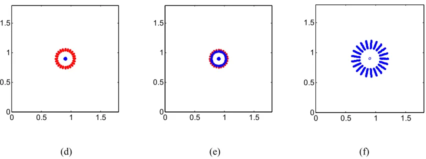
(d) (e) (f)
Figure 9.Space line charge trajectories above corona onset: (a) Positive corona onset; (b) Positive ions
261
moving away; (c) Positive ions return; (d) Negative corona onset; (
e)
Positive and negative ions moving262
on the contrary; (
f)
Negative ions return.263
4. Corona-loss analysis of bundle-sag conductors in the UHV corona cage
264
The calculation model proposed in this paper can also analyze the corona characteristics of the
265
conductor which has sag. In figure 10, the UHV corona cage set in Ping’an County, Xining City,
266
China (elevation 2,200 m), with a square cross-section (8 m × 8 m) and a total length of 35 m was
267
used. The corona cage is composed of a 25 m long measuring section and two protective sections on
268
each side of the measuring section, being 5 m long respectively. Based on the self-developed
269
integrated photoelectric corona loss measurement system, the test was carried out for bundle
270
conductors 4 × LGJ720 on a calm day without wind, the bundle spacing is 450mm,the equivalent
271
roughness coefficient value m is adopted as 0.75, PF is selected as 10, R=18.12mm, Rg =4.529mm.The
272
test ambient atmosphere pressure, temperature and relative humidity were 78.5-78.8kPa,
273
10.2-15.3°C and 68.8-82.8%, so μ+ and μ- are selected as 1.32×10⁻⁴ m2/(V∙s) and 1.65×10⁻⁴ m2/(V∙s)
274
respectively[22]. The diagrammatic sketch of conductors with sag in calculation model on front
275
view is shown in Figure 11, the changes trend of conductors at the axial direction is approximate to
276
the parabola in corona cage, coordinates matrix of bundle conductors with sag can be obtained by
277
the coordinate matrix’s shifting transformation and rotation transformation from long and straight
278
conductors by (33).
279
[ ]
11[ ][ ][ ]
1 2[ ][ ]
1 2 1X X
B Y A M M Y M M Z
Z
= = =
(33)
280
In (33), B is coordinates matrix of bundle conductors with sag, A is coordinates matrix of long and
281
straight conductors, M1 is matrix of shifting transformation, M2 is matrix of rotation transformation.
282
And the conductors with sag between 0.15m and 0.25m is calculated. As is shown in Figure 12,
283
test results are compared with calculation results. It can be seen that the corona losses calculated
284
around the vicinity of corona onset point have significant differences on different conductors’ sag
285
condition, however, as the applied voltage increases, the corona loss has the trend of closing to the
286
0 0.5 1 1.5 0
0.5 1 1.5
0 0.5 1 1.5 0
0.5 1 1.5
0 0.5 1 1.5 0
one certain value. And the conductors with sag=0.2m can approximate the practical situation more
287
accurately.
288
289
Figure 10. UHV corona cage at Ping’an
290
291
Figure 11. The conductor with sag in calculation model on front view
292
293
Figure 12. Corona losses with different sag of conductor
294
5. Conclusion
295
100 150 200 250 300 350 400 450
0 50 100 150 200 250
Co
ro
na
los
s (
w
/m)
Test voltage (kV) measurement
Based on helical charges, the Kaptzov assumption is used and the Deutsch assumption is
296
abandoned, and the inhomogeneity of space line charge emission and the actual structures of
297
conductor are taken into consideration. By introducing the measuring value of ion mobility and
298
simulating the processes including emission, transfer and recombination of space line charges, the
299
calculation method for 3-D corona loss of the conductor in the corona cage is established.
300
The test results of corona loss well coincide with the calculation results on single stranded
301
conductor and bundle-sag conductors in different corona cages. Compared with 2-D corona loss
302
calculation models, the model in this paper can take the electric-field nonuniformity along the axial
303
direction on the conductor surface, it is more accurate to analyze physical process of corona
304
discharge.
305
Acknowledgments: The authors would like to thank the reviewers of this paper for the useful comments. This
306
work is supported by National Natural Science Foundation of China (51577069) and the National Grid
307
Corporation of Science and Technology (Grant no. SGTYHT/15-JS-191).
308
Author Contributions: Shilong Huang established the 3-D calculation model for corona loss; Shilong Huang
309
analyzed the data; Yunpeng Liu, Shugang Liu, Daran Liu and Zhicheng Huang contributed
310
reagents/materials/analysis tools; Shilong Huang and Daran Liu wrote the paper.
311
Conflicts of Interest: The authors declare no conflict of interest.
312
References
313
1. Liu, Z.Y. Ultra-high voltage grid; China Economic Press: Beijing, China, 2005.
314
2. Zhang G.Z.; Cheng G.S.; Wan B.Q. Study on EM environment of UHV test line segment. High Voltage
315
Engineering. 2008, 34, 438-441.
316
3. Liu, Z.Y. Global Energy Internet; China Economic Press: Beijing, China, 2015.
317
4. Maruvada P S. Corona performance of high-voltage transmission lines; Research Studies Press Ltd: London,
318
2000.
319
5. Frans J.S.; Andrew M; Klas R. Evaluation, verification and operational supervision of corona losses in
320
Sweden. IEEE Trans on Power Delievery. 2007, 22, 1210-1217.
321
6. Anderson J.G.; Zaffanella L.E. Project UHV Test Line Research on the Corona Performance of a Bundle
322
Conductor at 1000 kV. IEEE Transactions on PAS.1970, 89, 1168-1178.
323
7. Vinh T.; Shih C.H.; King J.V.; Roy W.R. Audible Noise and Corona Loss Performance of 9-Conductor
324
Bundle for UHV Transmission Lines. IEEE Transactions on PAS, 1985,104, 2764-2770.
325
8. Juette G.W.; Zaffanella L.E. Radio Noise, Audible Noise, and Corona Loss of EHV and UHV Transmission
326
Lines Under Rain: Predetermination Based on Cage Tests. IEEE Transactions on PAS, 1970, 89, 1168-1178.
327
9. Kolcio N.; Caleca V.; Marmaroff S.J.; Gregory W.L. Radio-Influence and Corona-Loss Aspects of AEP
328
765-kV Lines. IEEE Transactions on PAS, 1969, 88, 1343-1355.
329
10. Chartier V.L.; Shankie D.F.; Kolcio N. The Apple Grove 750-kV Project: Statistical Analysis of Radio
330
Influence and Corona-Loss Performance of Conductors at 775 kV. IEEE Transactions on PAS, 1970, 89,
331
867-881.
332
11. Liu Y.P.; You S.H.; Wan Q.F. Design and realization of AC UHV corona loss monitoring system. High
333
Voltage Engineering, 2008, 34, 1797-1801.
334
12. Liu Y.P.; You S.H.; Wan Q.F. Research on UHV AC single circuit test line corona losses under rain.
335
Proceedings of the CSEE, 2010, 30, 114-119.
336
13. Clade J. J.; Gary C. H.; Lefevre C.A. Calculation of corona losses beyond the critical gradient in alternating
337
voltage. IEEE Trans on PAS,1969, 88,695-703.
14. Clade J. J.; Gary C. H. Predetermination of corona losses under rain: experimental interpreting and
339
checking of a method to calculate corona losses. IEEE Trans on PAS, 1970, 89,853-860.
340
15. Clade J. J.; Gary C. H. Predetermination of corona losses under rain: influence of rain intensity and
341
utilization of a universal chart. IEEE Trans on PAS. 1970, 89, 1179-1185.
342
16. Abdel S.M.; Abdel-Aziz E.Z. A charge simulation based method for calculating corona loss on AC power
343
transmission lines. Journal of Physics D: Applied Physics, 1994, 27, 2570.
344
17. Abdel S.M.; Abdel-Aziz E.Z. Corona power loss determination on multi-phase power transmission lines.
345
Electric power systems research, 2001, 58, 123-132.
346
18. Li W.; Zhang B.; He J.L. Influence of corona effect on ground level electrical field under EHV/UHV AC
347
transmission lines. High Voltage Engineering, 2008, 34, 2288-2294.
348
19. YOU S.H.; Lü F.C.; Liu Y.P. AC conductors' corona-loss calculation and analysis in corona cage',
349
Proceedings of the CSEE, 2012, 32, (1), pp.162-170.
350
20. Lü F.C.; You S. H.; Liu Y. P. AC conductors' corona-loss calculation and analysis in corona cage. IEEE
351
Trans on Power Delivery, 2012, 27, 877-885.
352
21. Hochberg D.; Edwards G.; Kephart T.W. Representing structural information of helical charge
353
distributions in cylindrical coordinates. Physical Review E.1997, 55, 3765.
354
22. Liu Y.P.; Huang S.L.; Zhu L. Influence of humidity and air pressure on the ion mobility based on drift tube
355
method. CSEE JPES, 2015, 1, 37-41.
356
23. Ministry of Machinery Industry of People’s Republic of China. Aluminium stranded conductors and
357
aluminium conductors steel-reinforced; Standards Press of China: Beijing, China, 1983.