Fast 3D Semantic Mapping on Naturalistic Road Scenes
Xuanpeng Li1,∗ , Dong Wang1, Huanxuan Ao1, Rachid Belaroussi2and Dominique Gruyer2
1 School of Instrument Science and Engineering, Southeast University, 210006 Nanjing, Jiangsu, China
2 COSYS/LIVIC, IFSTTAR, 25 allée des Marronniers, 78000 Versailles
* Correspondence: [email protected]
† This paper is an extended version of our paper published in LI, Xuanpeng, et al. Fast semi-dense 3D semantic mapping with monocular visual SLAM. In: Intelligent Transportation Systems (ITSC), 2017 IEEE 20th International Conference on. IEEE, 2017. S. 385-390.
1 2 3 4 5 6 7 8 9 10 11 12 13 14
Abstract: Fast 3Dreconstructionwith semantic informationon roadscenesis ofgreat requirementsfor
autonomousnavigation.Itinvolvesissuesofgeometryandappearanceinthefieldofcomputervision.Inthis
work,weproposeamethodoffast3Dsemanticmappingbasedonthemonocularvision.Atpresent,dueto
theinexpensivepriceandeasyinstallation,monocularcamerasarewidelyequippedonrecentvehiclesforthe
advanceddriverassistanceanditispossibletoacquiresemanticinformationand3Dmap. Themonocular
visualsequenceisusedtoestimatethecamerapose,calculatethedepth,predictthesemanticsegmentation,and
finallyrealizethe3Dsemanticmappingbycombinationofthetechniquesoflocalization,mappingandscene
parsing.Ourmethodrecoversthe3Dsemanticmappingbyincrementallytransferring2Dsemanticinformation
to3Dpointcloud.Andaglobaloptimizationisexploredtoimprovetheaccuracyofthesemanticmappingin
lightofthespatialconsistency.Inourframework,thereisnoneedtomakesemanticinferenceoneachframeof
thesequence,sincethemeshdatawithsemanticinformationiscorrespondingtosparsereferenceframes.It
savesamountsofthecomputationalcostandallowsourmappingsystemtoperformonline.Weevaluatethe
systemonnaturalisticroadscenes,e.g.,KITTIandobserveasignificantspeed-upintheinferencestageby
labelingonthemesh.
Keywords:3Dsemanticmapping;incrementalfusion;globaloptimization;realtime;naturalisticroadscenes 15
1. Introduction 16
Naturalistic scene understanding plays a key background role in most vision-based mobile robots. For 17
example, autonomous navigation in outdoor scenes asks for a rapid and comprehensive understanding of 18
surroundings for obstacle avoidance and path planning. Vehicle movement in limited temporal and spatial 19
contexts always requires knowledge of what something is, where it is located, and ego-vehicle’s surrounding. 20
Robotic maps, such as Occupancy grid map and OctoMap, traditionally provide geometric presentation of the 21
environment. However, they lack the correlation in data between map points and semantic knowledge; thus, they 22
could not be directly utilized in naturalistic road scenes. 23
Scene parsing is an important and promising step to address this issue. It benefits from the state-of-the-art 24
Deep Convolutional Neural Networks (DCNNs) which contributes to better performance of 2D pixel labeling 25
than traditional methods. Then, combined with the Simultaneous Localization and Mapping (SLAM) technology, 26
automobile could locate itself and meanwhile recognize surrounding objects in pixel-wise level. For instance, it 27
could make autonomous vehicle accomplish certain high-level tasks, such as “parking on the right free place” 28
and “stopping at the crosswalk”. This form of semantically annotated 3D representation provides mobile robots 29
with functions of understanding, interaction and navigation in various scenes. 30
Semantic segmentation has been an active topic for a long time. Most methods have focused on increasing 31
the accuracy of the semantic segmentation, and have seen major improvements [1–3]. However, they usually asks
32
for high-power computing resources, which is not suitable for the embedded platform. Several recent research 33
focuses on the balance between the computing cost and the accuracy of object detection, classification and 2D 34
pixel labeling [4,5]. They achieves a better performance with regards to the embedded and mobile platforms.
35
Compared to the SLAM technology with scaled sensors, such as stereo and RGB-D cameras, monocular 36
visual SLAM is a promising technology, because monocular vision is flexible, inexpensive, and most importantly, 37
widely equipped on most recent vehicles. Scaled sensors could provide reliable measurement in their specific 38
ranges, whereas they lack the capability of seamless switch between various-scale scenes such as indoor and 39
outdoor. And they normally need large storage resources. 40
Most man-made environments, e.g., road scenes, usually exhibit distinctive spatial relations among varied 41
classes of objects. Being able to capture, model and utilize these kinds of relations could enhance semantic 42
segmentation performance in the 3D semantic mapping [6]. In this paper, we exploit a monocular SLAM method
43
that provides cues of 3D spatial information and utilize state-of-the-art DCNN to build a 3D scene understanding 44
system towards road scenes. Moreover, a Bayesian 2D-3D transfer and a map regularization process are exploited 45
to generate a consistent reconstruction in the spatial and semantic context. 46
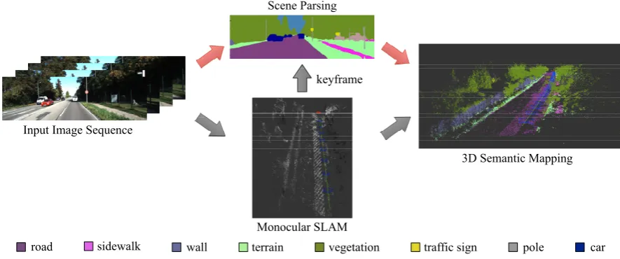
road
Input Image Sequence
Scene Parsing
Monocular SLAM
3D Semantic Mapping
sidewalk wall terrain vegetation traffic sign pole car keyframe
Figure 1. Overview of our system:From monocular image sequence, keyframes are selected to obtain its 2D semantic information, which then transfer to the 3D reconstruction to build the 3D semantic map.
In our monocular mapping system, the 3D map is incrementally reconstructed with a sequence of 47
automatically selected keyframes and corresponding semantic information. There is no need to label each 48
frame in a sequence, which could save a considerable amount of computation cost. We refer the reader to Figure1
49
for an illustration. Different from the frame skipping strategy proposed by Hermanset al.[7] and McCormacet
50
al.[8], our method could work well under fast camera motions. Since the 3D map should have global consistent
51
depth information, it could be regularized in term of spatial structures. The regularization is aimed to remove 52
distinctive outliers and makes components more consistent in the point cloud map, i.e., local points with same 53
semantic label should be approached in 3D space. Two datasets, Cityscapes [9] and KITTI [10], are used to
54
evaluate our approach. Several raw videos are taken to reconstruct 3D map with semantic labels. 55
This paper is presented as follows. In the following Section2, a review of the related work is given.
56
The problem formulation is presented in Section 3. The 3D semantic mapping is described in Section 4,
57
including the semantic segmentation, the monocular visual SLAM, the Bayesian incremental fusion and the 58
global regularization. Section5includes the results of 2D semantic inference and 3D semantic mapping. Finally,
59
Section6concludes the paper and discusses possible extensions of our work.
60
2. Related Work 61
Our work is motivated by [8] which contributes an indoor 3D semantic SLAM from the RGB-D input. It
62
aims towards a dense 3D map based on ElasticFusion SLAM [11] with semantic labeling. Pixel-wise semantic
63
information is acquired from a Deconvolutional semantic segmentation network [12] using the scaled RGB
64
information and the depth as the input. Depth information is also used to update surfel’s depth and normal 65
information to construct 3D dense map during loop closure. In addition, a previous work, SLAM++ [13], creates
66
In this paper, we make use of an incremental Bayesian fusion strategy with state-of-the-art visual SLAM and 68
semantic segmentation. 69
Visual SLAM usually contains sparse, semi-dense, and dense types depending on the methods of image 70
alignment. Feature-based methods only exploited limited feature points - typically image corners and blobs or 71
line segments, such as classic MonoSLAM [14] and ORB-SLAM [15,16]. They are not suitable for 3D semantic
72
mapping due to rather sparse feature points. In order to better exploit image information and avoid the cost on 73
calculation of features, direct dense SLAM system, such as the surfel-based dense slam, ElasticFusion [11] and
74
Dense Visual SLAM [17], have been proposed recently. Whereas, direct image alignment from these dense
75
methods is well-established for monocular, RGB-D and stereo sensors. Semi-dense methods like Large-Scale 76
Direct-SLAM (LSD-SLAM) [18] and Semi-direct Visual Odometry (SVO) [19] provide possibility to build a
77
synchronized 3D semantic mapping system. 78
Deep CNNs have proven to be effective in the field of image semantic segmentation. Longet al.[20] firstly
79
introduces an inverse convolution layer to realize an end-to-end training and inference. Then, the encoder-decoder 80
architectures with specified upsampling layers, such as max unpooling and deconvolutional layer, are proposed to 81
avoid the problem of separate step training in the FCN network and improve the accuracy [12,21]. Zhaoet al.[2]
82
exploits the capability of global context information through embedding various scenery context feature in a 83
pyramid structure. The fusion of varied scaled feature has been a popular strategy in the recent deep CNNs. The 84
cutting-edge method, namely, DeepLab series [1,3,5], combines atrous convolutions and atrous spatial pyramid
85
pooling (ASPP) to achieve a state-of-the-art performance on semantic segmentation. The early DeepLab models 86
have a reasonable accuracy but require much computation overhead. Recently proposed efficient convolution 87
neural network, such as MobileNets [22,23] boosts real-time performance of semantic segmentation without
88
losing the accuracy too much. The state-of-the-art DeepLab-v3+ [5] contains a simple effective decoder module
89
to refine the segmentation results especially along object boundaries. Furthermore, combining the encoder part of 90
MobileNet-v2 in its encoder-decoder structure, DeepLab-v3+ could achieve a better trade-off between precision 91
and runtime. 92
In the topic of scene understanding and mapping, recent research employ 3D priors of objects increasingly. 93
Salas-Morenoet al.[13] project 3D mesh of objects to the RGB-D frame in a graphical SLAM framework.
94
Valentinet al.[24] propose a triangulated meshed representation of the scene from multiple depth measurements
95
and exploit the Conditional Random Field (CRF) to capture the consistency of 3D object mesh. Kunduet al.[25]
96
exploit the CRF for joint voxels to infer the semantic information and occupancy. Sengupta and Sturgess [26]
97
use stereo camera, estimated pose and CRF to infer the semantic octree presentation of the 3D scene. Vineetet
98
al.[27] propose an incremental dense stereo reconstruction and semantic fusion technique to handle dynamic
99
objects in the large-scale outdoor scenes. Kochanovet al.[28] employ scene flow measurements to incorporate
100
temporal updates into the mapping of dynamic environment. Landrieuet al.[29] introduce a regularization
101
framework to obtain spatially smooth semantic labeling of 3D point clouds from a point-wise classification, 102
considering the uncertainty associated with each label. Gaussian Process (GP) is another popular method for map 103
inference. Jadidiet al.[30] exploit GP to learn the structural and semantic correlation between map points. This
104
technique also incorporates OcotoMap to handle sparse measurements and missing labels. In order to improve 105
the training and query time complexities of the GP-based semantic mapping, Ganet al.[31] further introduce a
106
Relevance Vector Machine (RVM) inference technique for efficient map query at any resolution. 107
Our semi-dense approach is also inspired by dense 3D semantic mapping methods [6,7,32,33] in both
108
indoor and outdoor scenes. The major contributions from these work involve the 2D-3D transfer and the map 109
regularization. Especially, Hermanset al.[7] propose an efficient 3D CRF to regularize 3D semantic mapping
110
consistently considering influence between neighbors of 3D points (voxels). In this work, we adopt a similar 111
strategy to improve the performance of the 3D semantic reconstruction in the road scenes. The key concepts are 112
• a 3D semantic mapping system based on the monocular vision,
113
• integration of monocular SLAM and scene parsing into 3D semantic representation,
114
• exploiting the correlation between semantic information and geometrical information to enforce spatial
115
• active sequence downsampling and sparse semantic segmentation so that to achieve a real-time performance 117
and reduce the storage. 118
Following the comparison in [27], we list the characteristics of our approach and some relative work in
119
TABLE1.
120
Table 1.Comparison with some related work: M = monocular camera, S/D = stereo/depth camera, L = Lidar, O = outdoor, I = incremental, SDT = sparse data structures, RT = real time
Method M S/D L O C I SDT RT
Huet al.[34] √ √ √ √ √
Senguptaet al.[32] √ √ √
Hermanset al.[7] √ √ √
Kunduet al.[25] √ √ √ √ √
Vineetet al.[27] √ √ √ √ √ √
Wolfet al.[6] √ √ √ √ √
McCormacet al.[8] √ √ √ √ √ √
Ours √ √ √ √ √ √
3. Problem Formulation 121
3.1. Notation 122
The target is to estimate the 3D semantic mapMcomprising of a pose-graph of keyframes with semantic
123
map taken from a monocular camera. LetIi:Ω→R3symbolize anH×WRGB image at the frame indexed
124
byi. Keyframes are extracted from image sequence in light of camera’s poseTjiat theiframe with respect to
125
previous keyframej. We define theith keyframe to be a tupleKi = (Ii,Di,Vi,Si), whereDi :ΩDi →Ris
126
the full-resolution inverse depth map associated with imageIi, andVi :ΩVi →Ris associated inverse depth
127
variance map. Depth map and variance are defined in the subset of pixels asΩDi ⊂Ωi, which means semi-dense,
128
only available for certain image regions of large intensity gradient. The symbolSi:ΩSi →Rrepresents the
129
full-resolution semantic map with maximum probability of object class from the semantic segmentation process. 130
The keyframes are consecutively stacked in a pose-graphG= (V,E), whereV ={K0, . . . ,Kn}is the set
131
of keyframes andE ={Sij∈Sim(3):Ki,Kj ∈ V }is the set of constraint factors. EachSji= (Tji,sji)consists
132
of a camera’s poseTji = (R t0 1)from keyframeito keyframe j, and scale factorsji >0. In reference to world
133
frameW, normally regarded as the first keyframeK0, the pose of the keyframe indexed byiis denoted asTiW.
134
For a sequence of keyframes (nkeyframes), we get thenth keyframe’s poseTnW=∏n1Tkk−1.
135
The 3D mapMis reconstructed by the projection of the inverse depth map of all keyframes, where each
136
3D pointPcan be labeled as one of the solid semantic objects in the label spaceL={l1,l2, . . . ,lk}likeRoad,
137
Building,Tree, etc. We useX={X1,X2, . . . ,XM}to denote the set of random variables corresponding to the 138
3D pointsPi:i∈ {1, . . . ,M}, where each variableXi∈Xtake a valuelifrom the predefined label spaceL.
139
3.2. 3D semantic mapping 140
Our target is to build a 3D semantic map with semi-dense and consistent label information online while the image sequences are captured by a moving monocular forward camera. Given an image sequence, the inference of the 3D semantic map is regarded as:
M∗ =argmaxMP(M|G), (1)
which can be estimated by the maximum a-posterior (MAP). Compared to the model used in [25], our observation
141
is continuously updating, not all existing measurements. Thus, we adopt an incremental fusion strategy to 142
estimate the 3D semantic map by incorporating new arriving keyframes. Correspondingly, the approach is 143
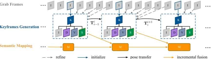
decoupled into three separately running processes as shown in Figure2.
Grab Frames
K
M
I I I I I I I I I I I I I I I
S
I D V
refine initialize
I
M M
S
I D V I D V S K K
…
…
…
incremental fusion Keyframes Generation
Semantic Mapping
pose transfer
…
…
…
Ti
i−1 Tii+1
Figure 2. Framework of our method: The input is the sequence of the RGB frames, denoted asI. There are three separate processes, a keyframe selection process, a 2D semantic segmentation process , and a 3D reconstruction with semantic optimization process. KeyframesKare conditionally extracted from the sequence based on the distance between the poses. The following frames refine the depth map and the variance map of each keyframe until new keyframe is extracted. The 2D semantic segmentation module predicts the pixel-level class of the new-arriving keyframe. Finally, the keyframes are incrementally explored to reconstruct the 3D map with semantic labeling and then it is regularized by a dense CRF.
In the system, the monocular SLAM process maintains and tracks on a global map of the environment, which 145
contains a number of keyframes connected by pose-pose constraints with associated probabilistic semi-dense 146
depth maps. It runs in real-time on a CPU. Represented as point clouds, the map gives a semi-dense and highly 147
accurate 3D reconstruction of the environment. Meanwhile, the second process of the 2D semantic segmentation 148
generates the pixel-level classification on the extracted keyframes. A fast deep CNN model is explored to predict 149
the semantic information on a GPU. In addition, an incremental fusion process for the semantic label optimization 150
is operated in a parallel way. It builds a local optimal correspondence between semantic labeling and voxels in the 151
3D point cloud. To obtain a globally optimal 3D semantic segmentation, we attempt to make use of information 152
of neighboring 3D points, involving the distance, color similarity and semantic label. It updates voxel’s position 153
and corresponding semantic label, which gives a globally consistently 3D semantic map. 154
4. 3D Semantic Mapping 155
4.1. 2D Scene Parsing 156
We explore the DeepLab-v3+ deep neural network proposed by Chenet al.[5]. Two important components
157
in the DeepLab series are the atrous convolution and atrous spatial pyramid pooling (ASPP), which enlarge 158
the field of view of filters and explicitly combine the feature maps at multiple scales. The improvement in the 159
DeepLab-v3+ involves the encoder-decoder structure and the augmentation of ASPP module with image-level 160
feature. The former is able to capture sharper object boundaries by regaining the spatial information, while the 161
latter encodes multi-scale contextual information to capture long range information. These contributions make 162
DeepLab successfully handle both large and small objects and achieve a better trade-off between precision and 163
run-time. 164
For the semantic segmentation of road scenes, we exploit the Cityscapes dataset and the KITTI dataset and 165
adopt the predefined 19-class label spaceL={l1,l2, . . . ,l19}, which containsRoad,Sidewalk,Building,Wall,
166
and so on. We use all semantic annotated images in the Cityscapes dataset for training and fine-tune the model 167
with the KITTI dataset. 168
Note that there is not any depth information involved in the training process. In the inference, we keep the 169
original resolution of input image according to different datasets. 170
4.2. Semi-Dense SLAM 171
We explore LSD-SLAM to track camera’s trajectory and build consistent, large-scale maps of the 172
a scale-aware image alignment algorithm to directly estimate the similarity transform between two keyframes 174
against different scale environments, such as office rooms (indoor) and urban roads (outdoor). The second one is 175
that it is a probabilistic approach to incorporate noise on the estimated depth maps into the tracking based on the 176
propagation of uncertainty. Moreover, it could integrate easily with different kinds of sensors like monocular, 177
stereo and panoramic cameras for various applications. These features are of benefit to a reliable tacks and maps 178
even in challenging surroundings. 179
LSD-SLAM has three major components: tracking, depth map estimation and map optimization. Spatial 180
regularization and outlier removal are incorporated in the estimation of depth map with small-baseline stereo 181
comparisons. In addition, a direct, scale-drift aware image alignment is carried on these existing keyframes to 182
detect scale-drift and loop closures. Due to the inherent correlation between the depth map and the tracking 183
accuracy, depth residual is used to estimate the similarity transformsim(3)constraints between keyframes.
184
Consequently, a 3D point cloud map is built based on a set of keyframes with the estimated depth maps via 185
minimizing the error of image alignment. The map is continuously optimized in the background using ag2o
186
pose-graph optimization. The approach runs in 25Hz on an Intel i7 CPU. More details like keyframe selection 187
and depth estimation should be referred to the work [18].
188
4.3. Incremental Fusion 189
There might be a large amount of inconsistent 2D semantic labels between consecutive frames, due to 190
the noise of sensors, the complexity of environments in the real world and the failure of scene parsing model. 191
Incremental fusion of semantic label from the stacked keyframes allows associating probabilistic label in a 192
Bayesian way, when combining with the depth map propagation between keyframes in the LSD-SLAM. We will 193
give the details about the incremental semantic fusion with the depth estimation as follows. 194
The camera projection transformation functionπ(·):R3→R2is defined as
p=π(P) = [αx
z +cx,β y z+cy]
T, (2)
which maps a pointP= [x,y,z]Tin 3D space into a 2D pointp = [x0,y0]Ton the digital image planeIiin
the camera coordinate system. Since this projection function is nonlinear, for the computation efficiency, the transformation should be augmented into the homogeneous coordinate system, which is defined as
ph=
x0h y0h z0h
=
α 0 cx 0
0 β cy 0
0 0 1 0
x y z 1
=K[I0]Ph, (3)
where the matrixKis referred to as the camera matrix. Given a 3D pointPWin the world reference system, the
mapping to image planeIiin the homogeneous reference system is calculated as
ph=KTWi PWh, (4)
whereTWi the pose of the camera in the world reference system. Then, we get Euclidean coordinatesp =
195
[x0h/z0h,yh0/z0h]Tfrom the homogeneous coordinates. From this point on, any pointpandPis assumed to be in
196
homogeneous coordinates and thus we drop thehindex, unless stated otherwise.
197
Correspondingly, given the inverse depth estimationdˆfor a pixelp= [x0,y0]TinIiof the keyframeKi, we
also have an inverse projection function below:
P=π−1(p, ˆd) = [x
0/ ˆd−c
x/ ˆd
α ,
y0/ ˆd−cy/ ˆd
β ,
1 ˆ d]
T, (5)
wheredˆ=Di(p)corresponds to the pointpexisting in the depth mapDi, which projects the 2D pixel point into
continuously refined using its following frames until new keyframe is defined. In reference to Equation4and5, we can derive the 3D point in the world reference system as follows:
PW=TWi
−1
π−1(p,Di(p)), (6)
where the homogeneous transformation matrix has the property:TWj −1=TW
j . 198
Once a new frame is chosen to become a keyframeKj, its depth mapDjis initialized by projecting points
from previous keyframe into it. The information of existing, close-by keyframes is propagated to new keyframe for its initialization and semantic probabilistic refinement. The point in the depth map of new keyframe is obtained by
p=KTiWTijPW ∈Ij. (7)
Here, we have a Gaussian distributed transformation between keyframes, regarded asp∈ Ii→PW→p∈ Ij.
199
The class label corresponding to a 3D pointPis denoted asX :P→l ∈ L. Note that the labelSkyis
200
removed fromLfor the 3D semantic mapping. Our target is to obtain the independent probability distribution of
201
each 3D point over the class labelsP(X|Ki
0)given a sequence of existing keyframesK0i ={K0,K1, . . . ,Ki}in
202
the pose-graphG.
203
We explore a recursive Bayesian fusion to refine the corresponding probability distribution of 3D points with new keyframe’s update:
P(X|Ki0) = 1 Zi
P(Ki|Ki0−1,X)P(X|Ki0−1), (8)
withZi=P(Ki|K0i−1). Applying the first-order Markov assumption top(Ki|Ki0−1,X), then we have:
P(X|Ki 0) =
1 Zi
P(Ki|X)P(X|Ki−1 0 ) =
1 Zi
p(Ki)P(X|Ki) P(X) P(X|K
i−1
0 ). (9)
We assume that P(X)does not change over time and there is no need to calculate the normalization factor
204
P(Ki)/Ziexplicitly.
205
According to the formulations above, the semantic probability distribution of all given keyframes can be recursively updated as follows:
P(X|Ki
0)∝P(X|Ki)P(X|Ki0−1). (10) The incremental fusion can refine the semantic label of the points in the 3D space based on the pose-graph 206
of keyframes. It could handle the inconsistent 2D semantic labels, even though its performance relies on the 207
depth estimation. In addition, map geometry is another useful feature which could improve the performance of 208
the 3D semantic mapping further. The following section describes how we use the dense CRF to regularize the 209
3D semantic map by exploring the map geometry, which could propagate semantic information between spatial 210
neighbors. 211
4.4. Map Regularization 212
The dense CRF is widely used in the 2D semantic segmentation to enhance the performance of semantic 213
segmentation. Some previous works [6,7,32] seek its application on the 3D map to model contextual relations
214
between various class labels in a fully connected graph. It is a heuristic approach that assume the influence 215
between neighbors should be proportional to their distance, visual and geometrical similarity [7].
216
The CRF model is defined as a graph composed of unary potentials as nodes and pairwise potentials as 217
edges, but the size of the model makes traditional inference algorithms impractical. Thanks to Krahenbuhl 218
and Koltun’s work [35], a highly efficient approximate inference algorithm is proposed to handle this issue by
219
defining the pairwise edge potentials as a linear combination of Gaussian kernels. We apply the efficient inference 220
Assume the 3D semantic mapMcontainingM3D points is defined as a random field. A CRF(M,X)is characterized by a Gibbs distribution as follows:
P(X|M) = 1
Z(M)exp(−E(X|M)), (11)
whereE(X|M)is the Gibbs energy andZ(M)is the partition function. The maximum a posteriori (MAP)
labeling of the random field is
X∗=argmaxl∈LP(X|M) =argminl∈LE(X|M), (12)
which is converted into minimizing the Gibbs energy by the mean-field approximation and message passing 222
scheme. 223
We employ the associative hierarchical CRF [32,36] which integrates the unary potentialψi, the pairwise
potentialψi,jand the higher order potentialψcinto the Gibbs energy at different levels of the hierarchy (voxels
and supervoxels) given by:
E(X|C;`) =
∑
i
ψi(Xi|C) +
∑
i<jψi,j(Xi,Xj|C;θ) +
∑
c
ψc(Xc|c) (13)
by the indexesi,j∈ {1, . . . ,M}correspond to different 3D pointsPi,Pjin the 3D mapM.
224
Unary Potential: The unary potentialψi(·)is defined as the negative logarithm of the probabilistic label for a given 3D point:
ψi(Xi|C) =−log(P(Xi →ł|Kt0)). (14)
This term means the cost of 3D point Pi taking an object label l ∈ Lbased on the incremental semantic
225
probabilistic fusion above. The output of the unary potential for each point is produced independently, and thus, 226
the MAP labeling produced by the unary potential alone is generally inconsistent. 227
Pairwise Potentials: The pairwise potentialψi,j(·)is modeled to be a log-linear combination ofmGaussian edge potential kernels:
ψi,j(Xi,Xj|C;θ) =µ(Xi,Xj)
∑
mω(m)k(m)(fi,fj;θ), (15)
whereµ(·)is a label compatibility function corresponding to the Gaussian kernel functionsk(m)(fi,fj).fdenotes
the feature vector for the 3D pointPincluding the position, the RGB appearance and the surface normal vector
of the reconstructed surface. Andµ(·)is a Potts model given by:
µ(l,l0) = [l6=l0] = (
1 l6=l0
0 l=l0 . (16)
This term is defined to encourage the consistency over pairs of neighboring points for the local smoothness of the 3D semantic map. We employ two Gaussian kernels for the pairwise potentials following the previous
work [7]. The first one is an appearance kernel as follows:
k(1)(fi,fj;`) =exp −
|Pi−Pj|2
2θ2P,c
−|ci−cj|
2
2θc2
!
, (17)
where cis the RGB color vector of the corresponding 3D points. This kernel is used to build long range
228
connections between 3D points with a similar appearance. 229
The second one, a spatial smoothness kernel, is defined to enforce a local, appearance-agnositc smoothness among 3D points with similar normal vectors.
k(2)(fi,fj;θ) =exp −
|Pi−Pj|2
2θP2,n
−|ni−nj|
2
2θn2 !
wherenare the respective surface normals. The surface normal are computed using the Triangulated Meshing 230
using Marching Tetrahedra (TMMT) proposed in [32]. Note that the original method is towards producing a
231
dense labeling with the stereo vision. Since the LSD-SLAM only generates semi-dense 3D point clouds, we 232
modify the TMMT to extract a triangulated mesh within limited ranges of short distance between 3D points. 233
High Order Potential: The higher order termψc(Xc|c)encourages the 3D points (voxels) in the given
segment to take the same label and penalizes partial inconsistency of supervoxels as described in [36]. It is
defined as
ψc(Xc|c) =minl∈L(γcmax,γlc+klcNcl), (19)
where γcl represents the cost if all voxels in the segment take the label l. Ncl = ∑i∈cδ is the number of
234
inconsistent 3D points with the labellwhich is penalized with a factorkc, regarded as the inconsistency cost.
235
All parametersθP,c,θc,θP,n,θn,θP,s,θsspecify the range in which points with similar features affect each
236
other, respectively. They can be obtained using piece-wise learning. 237
5. Experiments and Results 238
We demonstrate the performance of our approach on the KITTI dataset [10], which contains a variety of
239
urban scene sequences involving lots of moving objects in various lighting conditions. It consists of various 240
datasets, such as the semantic dataset, the odometry dataset, and the detection dataset. Thus, it is very challenging 241
for the 3D reconstruction. The KITTI dataset contains a 2D semantic segmentation data of 200 labeled 242
training images and 200 test images1. Its data format and metrics conform with the Cityscapes dataset [9].
243
The Cityscapes dataset involves 19 classes within high quality pixel-level annotations of 5000 images with a 244
resolution of2048×1024, including 2975 training images, 500 validation images, and 1525 testing images. In
245
our experiment, we train the model on the Cityscapes and then tune it on the KITTI taking the volume size of 246
dataset into account. 247
For the training of 2D semantic segmentation model, various encoder models in the DeepLab-v3+ are 248
evaluate includingResNet,Xception, andMobileNet. And we find that the “poly” stochastic gradient descent is
249
better than the “step” one on these datasets. TheTensorFlowlibrary is employed to do the training and inference
250
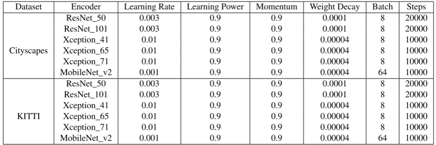
on the workstation with 4 Nvidia Titan X GPU cards. The hyper-parameters used in training are set corresponding 251
to the datasets and models as shown in Table2.
252
Table 2.Hyper-parameters used in the training step
Dataset Encoder Learning Rate Learning Power Momentum Weight Decay Batch Steps
ResNet_50 0.003 0.9 0.9 0.0001 8 20000
ResNet_101 0.003 0.9 0.9 0.0001 8 20000
Xception_41 0.01 0.9 0.9 0.00004 8 10000
Cityscapes Xception_65 0.01 0.9 0.9 0.00004 8 10000
Xception_71 0.01 0.9 0.9 0.00004 8 10000
MobileNet_v2 0.001 0.9 0.9 0.00004 64 10000
ResNet_50 0.003 0.9 0.9 0.0001 8 20000
ResNet_101 0.003 0.9 0.9 0.0001 8 20000
Xception_41 0.01 0.9 0.9 0.00004 8 10000
KITTI Xception_65 0.01 0.9 0.9 0.00004 8 10000
Xception_71 0.01 0.9 0.9 0.00004 8 10000
MobileNet_v2 0.001 0.9 0.9 0.00004 64 10000
We benchmark the performance of our semantic mapping system on the KITTI odometry dataset2. There
253
are 22 sequences with the consecutive RGB frames, in which there are 11 sequences with the ground-truth poses 254
for evaluation. The scenes contain serious illumination change, moving objects like persons and vehicles, and 255
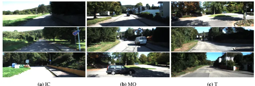
some turns as shown in Figure3. These road-scene frames involves two resolutions1242×375and1226×370. 256
Our system runs on an Intel Core i7-5960K CPU and a NVIDIA Titan X GPU for online process. 257
Since the KITTI sequences are mostly captured in 10 Hz, it is highly below the normal speed requirements 258
of LSD-SLAM about 60 Hz. In addition, the LSD-SLAM is hard to handle severe turning when the platform 259
moves. Due to the limit of the monocular LSD-SLAM, we choose 6 sequences to evaluate. 260
In the following sections, we show some qualitative results for our approach in5.1and the quantitative
261
results of our evaluation are presented in5.2, in which we also make the runtime analysis on our semantic
262
mapping approach. 263
5.1. Qualitative Results 264
First, we present some qualitative results of the KITTI semantic dataset in Figure4. Then, we use the
265
trained model to make prediction on the KITTI odometry dataset, and the results are exemplified as shown in 266
Figure5.
267
Take the sequenceodometry_03as an example of our semantic mapping approach. The sequence consists
268
of 801 RGB frames on a urban road of about 560m and a camera calibration file. Figure6shows the semantic
269
reconstruction with a close-up view including large-scale annotations such asroad,buildingand even small-scale
270
objects liketraffic signs. Note we discard some keyframes at the beginning, due to random initialization of
271
LSD-SLAM. 272
·
(a)IC (b)MO (c)T
Figure 3.Instances in theodometry_03sequence. IC: Illumination Change, MO: Moving Objects, T: Turns
(a)Raw Image (b)Prediction (c)Ground Truth
Figure 5.Instances of 2D semantic segmentation in the KITTI odometry set
Figure 6.Qualitative results of 3D semantic mapping from the sequenceodometry_03. Our approach not only reconstructs and labels entire outdoor scenes that include roads, sidewalks and buildings, but also accurately recovers thin objects such as traffic signs and trees.The close-up views show the details of the map.
5.2. Quantitative Results 273
For the quantitative performance of our approach, we focus on the 2D semantic segmentation and the 274
runtime of the entire system, since the 3D reconstruction mainly depends on the LSD-SLAM method. 275
Semantic Segmentation: Table3shows the quantitative results of 2D semantic segmentation based on different DeepLab-v3+ models on the KITTI datasets. We evaluate these models by the mean intersection/union (mIOU) score, the model size, and the computational runtime. The mIOU score is defined as
mIOU= 1
|L|
|L|
∑
i=1TPi/(TPi+FPi+FNi) (20)
in terms of the True/False Positives/Negatives for a given classi. We do not resize the image to evaluate the
276
models here. Whereas, for the 3D semantic mapping process, we need to half resize the input images in order to 277
make a trade-off between accuracy and computational speed. 278
During the training process, these models are initialized with the checkpoints pre-trained from various 279
datasets including ImageNet [37] and MS-COCO [38]. In the training step on the Cityscapes dataset, we directly
280
use the ImageNet-pretrained checkpoints as the initialization. Note we employ theMobileNet_v2based model
281
which has been pre-trained on MS-COCO dataset, and theXception_71based model has been pre-trained on
282
both ImageNet and MS-COCO datasets. These pre-trained models can be accessed from the github3.
283
Table 3. Quantitative results of various encoder parts of DeepLab-v3+ on the Cityscapes and the KITTI. I: ImageNet, M: MS-COCO, C: Cityscapes
Dataset Encoder Crop Size mIOU[0.5:0.25:1.75] Pb Size (MB) Runtime (s) I M C
ResNet_50 769 63.92 107.8 - √
ResNet_101 769 69.88 184.1 - √
Xception_41 769 68.5 113.4 - √
Cityscapes Xception_65 769 78.73 165.7 5.0 √
Xception_71 769 80.24 167.9 - √ √
MobileNet_v2 513 70.7 8.8 0.8 √
MoblieNet_v2 769 70.9 8.8 0.8 √
ResNet_50 769 51.35 107.8 0.9 √ √
ResNet_101 769 57.12 184.1 1.1 √ √
Xception_41 769 54.2 113.4 0.88 √ √
KITTI Xception_65 769 64.8 165.6 1.13 √ √
Xception_71 769 66.2 167.9 1.26 √ √ √
MobileNet_v2 513 57.74 8.8 0.2 √ √
MobileNet_v2 769 60.73 8.8 0.2 √ √
Then we fine-tune the models on the KITTI dataset by using the pre-trained Cityscapes model. The 284
Xception_71based model performs the best mIOU performance but a rather slow computational speed. The 285
MobileNet_v2 based model has a moderatemIOU, the smallest file size and the fastest speed. Note the 286
MobileNet_v2based model does not employ ASPP and decoder modules for fast computation. Considering the 287
balance between computational speed and accuracy, we choose theMobileNet_v2based model to carry out the
288
2D semantic segmentation in our approach. Table4shows the performance of theMobileNet_v2based model on
289
the VAL/TEST split of the KITTI dataset. 290
Table 4.Results of our selected model on the val/test of the KITTI datasets.
method road side
w
alk
b
uilding
w
all
fence pole traf
fic
light
traf
fic
sign
v
egetation
terrain sky person rider car truck bus train motorc
ycle
bic
ycle
IoU
VAL 95.7 73.9 87.1 38.1 44.2 42.7 48.6 60.3 89.1 52.3 90.1 70.1 36.5 89.1 44.6 62.2 37.4 36.1 67.7 60.3 TEST 96.1 73.7 86.2 37.9 41.4 40.1 50.3 58.3 90.2 66.8 91.3 72.4 40.3 91.8 33.7 46.4 37.1 46.0 62.4 60.9
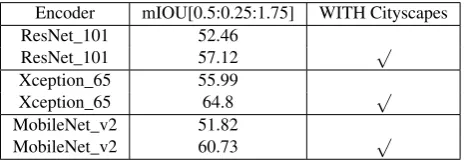
We also make the test regarding to the effect of pre-training on the Cityscapes dataset. In Table5, the
291
salience has been illustrated on training theXception_65andMobileNet_v2models. The Cityscapes pre-trained
292
models could greatly improve the performance of 2D semantic segmentation on the KITTI dataset. 293
Table 5.Performance of 2D semantic segmentation with/without the Cityscapes. Using the pre-trained Cityscapes model, the accuracy of 2D semantic segmentation could be greatly improved on the KITTI semantic data.
Encoder mIOU[0.5:0.25:1.75] WITH Cityscapes
ResNet_101 52.46
ResNet_101 57.12 √
Xception_65 55.99
Xception_65 64.8 √
MobileNet_v2 51.82
MobileNet_v2 60.73 √
Note that towards the 3D semantic mapping, since we use a novel monocular 3D mapping different from 294
the other related work, it is not easy to make quantitative comparison here. Kunduet al.’s work [25] propose
295
a joint semantic segmentation and 3D reconstruction from monocular video, but it is an offline approach with 296
different 3D representation in the form of a 3D volumetric semantic + occupancy map. 297
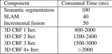
Runtime and Storage:As shown in Table6, our SLAM system runs about 40ms on average to process each 298
segmentation process requires about 100ms to infer 2D semantic information parallel upon the keyframes, and 300
the incremental fusion process needs 50ms on average. In the experiments, we find the SLAM process normally 301
selects a keyframe from more than every 4 frames. It keeps enough timing for the 2D semantic segmentation and 302
the incremental fusion during the 3D semantic mapping. Thus, our approach could run in real-time. Moreover, 303
considering the speed of moving platform, in case of the speed of 60KMH, the semantic segmentation process on 304
selected keyframes corresponds to a distance about 2 meters, which is not too sparse for an urban scene. 305
The lower part of this table shows the ranges of the CRF timing with different configurations due to the 306
different size of point clouds when testing various sequences in the experiments. The CRF update runs offline 307
due to slow inference speed on the CPU. Thus, it is only applied once at the end of the sequence. Optimized 308
GPU implementation can be studied in future to realize the online CRF update. 309
Table 6.Timing results. The table lists the operation time for different components of our system. Times of three core components are averaged over all sequences and the CRF timings depends on the iterations and the point cloud sizes.
Component Consumed Time (ms)
Semantic segmentation 100
SLAM 40
Incremental fusion 50
3D CRF 1 Iter. 800-2000
3D CRF 2 Iter. 1200-2400
3D CRF 3 Iter. 1500-3000
3D CRF 4+ Iter. >2000
Taking theodometry_03sequence as example, our approach acquires 114 keyframes with 2.8E+07 3D
310
points. Compared to the total 801 frames, the system utilizes only about1/7frames for mapping. Note that
311
smaller values of the parametersKFDistWeight andKFUsageWeight could give more constraints between
312
keyframes so that to achieve more accurate mapping. But it has a rather limited influence on the number of 313
keyframes, the number of 3D points and the size of storage. 314
6. Conclusions 315
We have presented a fast monocular 3D semantic mapping system which runs on a CPU coupled with a 316
GPU. An incremental fusion method is introduced to combine 2D semantic segmentation and 3D reconstruction 317
online. We exploit a state-of-the-art deep CNN to realize the scene parsing in the road contexts. Direct monocular 318
SLAM provides a quick 3D mapping based on selected keyframes and corresponding depth estimation. Since 319
the semantic segmentation only runs and propagates on the keyframes, this reduces the computational cost and 320
improves the accuracy of semantic mapping. The offline regularization with a CRF model can enhance the 321
mapping further. 322
Since the original LSD-SLAM is hard to handle the cases of sharp turns which are frequent in ordinal 323
driving, our system is not stable in such conditions. In addition, semi-dense 3D reconstruction should be replaced 324
by a dense model. In future work, we plan to introduce several state-of-the-art SLAM methods to improve 325
the initialization and resistance to serious movements, i.e., rotations. Research on how labeling boosts 3D 326
reconstruction of SLAM would be an interesting direction. The optimization of the regularization module would 327
be another effective direct on the wide-range mapping. 328
Funding:This research was funded by the Natural Science Foundation of Jiangsu Province grant number No. BK20160700 329
and No. BK20170681. 330
Conflicts of Interest:The authors declare no conflict of interest. The funders had no role in the design of the study; in the 331
collection, analyses, or interpretation of data; in the writing of the manuscript, or in the decision to publish the results. 332
333
1. Chen, L.C.; Papandreou, G.; Kokkinos, I.; Murphy, K.; Yuille, A.L. Semantic image segmentation with deep 334
2. Zhao, H.; Shi, J.; Qi, X.; Wang, X.; Jia, J. Pyramid scene parsing network. IEEE Conf. on Computer Vision and 336
Pattern Recognition (CVPR), 2017, pp. 2881–2890. 337
3. Chen, L.C.; Papandreou, G.; Kokkinos, I.; Murphy, K.; Yuille, A.L. Deeplab: Semantic image segmentation with 338
deep convolutional nets, atrous convolution, and fully connected crfs. IEEE transactions on pattern analysis and
339
machine intelligence2018,40, 834–848. 340
4. Zhao, H.; Qi, X.; Shen, X.; Shi, J.; Jia, J. ICNet for Real-Time Semantic Segmentation on High-Resolution Images. 341
European Conference on Computer Vision. Springer, 2018, pp. 418–434. 342
5. Chen, L.C.; Zhu, Y.; Papandreou, G.; Schroff, F.; Adam, H. Encoder-decoder with atrous separable convolution for 343
semantic image segmentation. European Conference on Computer Vision, 2018, pp. 833–851. 344
6. Wolf, D.; Prankl, J.; Vincze, M. Fast semantic segmentation of 3D point clouds using a dense CRF with learned 345
parameters. 2015 IEEE International Conference on Robotics and Automation (ICRA), 2015, pp. 4867–4873. 346
7. Hermans, A.; Floros, G.; Leibe, B. Dense 3d semantic mapping of indoor scenes from rgb-d images. 2014 IEEE 347
International Conference on Robotics and Automation (ICRA), 2014, pp. 2631–2638. 348
8. McCormac, J.; Handa, A.; Davison, A.; Leutenegger, S. SemanticFusion: Dense 3D semantic mapping with 349
convolutional neural networks. Robotics and Automation (ICRA), 2017 IEEE International Conference on. IEEE, 350
2017, pp. 4628–4635. 351
9. Cordts, M.; Omran, M.; Ramos, S.; Rehfeld, T.; Enzweiler, M.; Benenson, R.; Franke, U.; Roth, S.; Schiele, B. The 352
cityscapes dataset for semantic urban scene understanding. Proceedings of the IEEE conference on computer vision 353
and pattern recognition, 2016, pp. 3213–3223. 354
10. Geiger, A.; Lenz, P.; Urtasun, R. Are we ready for autonomous driving? the kitti vision benchmark suite. Computer 355
Vision and Pattern Recognition (CVPR), 2012 IEEE Conference on. IEEE, 2012, pp. 3354–3361. 356
11. Whelan, T.; Salas-Moreno, R.F.; Glocker, B.; Davison, A.J.; Leutenegger, S. ElasticFusion: Real-time dense SLAM 357
and light source estimation.The International Journal of Robotics Research2016,35, 1697–1716. 358
12. Noh, H.; Hong, S.; Han, B. Learning Deconvolution Network for Semantic Segmentation. The IEEE International 359
Conference on Computer Vision, 2015. 360
13. Salas-Moreno, R.F.; Newcombe, R.A.; Strasdat, H.; Kelly, P.H.; Davison, A.J. Slam++: Simultaneous localisation 361
and mapping at the level of objects. Proceedings of the IEEE conference on computer vision and pattern recognition, 362
2013, pp. 1352–1359. 363
14. Davison, A.J.; Reid, I.D.; Molton, N.D.; Stasse, O. MonoSLAM: Real-time single camera SLAM.IEEE transactions
364
on pattern analysis and machine intelligence2007,29, 1052–1067. 365
15. Mur-Artal, R.; Montiel, J.M.M.; Tardos, J.D. ORB-SLAM: a versatile and accurate monocular SLAM system.IEEE
366
Transactions on Robotics2015,31, 1147–1163. 367
16. Mur-Artal, R.; Tardós, J.D. Orb-slam2: An open-source slam system for monocular, stereo, and rgb-d cameras. IEEE
368
Transactions on Robotics2017,33, 1255–1262. 369
17. Kerl, C.; Sturm, J.; Cremers, D. Dense visual SLAM for RGB-D cameras. Intelligent Robots and Systems (IROS), 370
2013 IEEE/RSJ International Conference on. Citeseer, 2013, pp. 2100–2106. 371
18. Engel, J.; Schöps, T.; Cremers, D. LSD-SLAM: Large-scale direct monocular SLAM. European Conference on 372
Computer Vision, 2014, pp. 834–849. 373
19. Forster, C.; Zhang, Z.; Gassner, M.; Werlberger, M.; Scaramuzza, D. Svo: Semidirect visual odometry for monocular 374
and multicamera systems. IEEE Transactions on Robotics2017,33, 249–265. 375
20. Long, J.; Shelhamer, E.; Darrell, T. Fully convolutional networks for semantic segmentation. Proceedings of the 376
IEEE Conference on Computer Vision and Pattern Recognition, 2015, pp. 3431–3440. 377
21. Badrinarayanan, V.; Kendall, A.; Cipolla, R. SegNet: A Deep Convolutional Encoder-Decoder Architecture for Image 378
Segmentation. IEEE Transactions on Pattern Analysis and Machine Intelligence2017, pp. 2481–2495. 379
22. Howard, A.G.; Zhu, M.; Chen, B.; Kalenichenko, D.; Wang, W.; Weyand, T.; Andreetto, M.; Adam, H. Mobilenets: 380
Efficient convolutional neural networks for mobile vision applications.arXiv preprint arXiv:1704.048612017. 381
23. Sandler, M.; Howard, A.; Zhu, M.; Zhmoginov, A.; Chen, L.C. MobileNetV2: Inverted Residuals and Linear 382
Bottlenecks. Proceedings of the IEEE Conference on Computer Vision and Pattern Recognition, 2018, pp. 4510–4520. 383
24. Valentin, J.P.; Sengupta, S.; Warrell, J.; Shahrokni, A.; Torr, P.H. Mesh based semantic modelling for indoor and 384
outdoor scenes. Computer Vision and Pattern Recognition (CVPR), 2013 IEEE Conference on. IEEE, 2013, pp. 385
2067–2074. 386
25. Kundu, A.; Li, Y.; Dellaert, F.; Li, F.; Rehg, J.M. Joint semantic segmentation and 3d reconstruction from monocular 387
26. Sengupta, S.; Sturgess, P. Semantic octree: Unifying recognition, reconstruction and representation via an octree 389
constrained higher order MRF. Robotics and Automation (ICRA), 2015 IEEE International Conference on. IEEE, 390
2015, pp. 1874–1879. 391
27. Vineet, V.; Miksik, O.; Lidegaard, M.; Nießner, M.; Golodetz, S.; Prisacariu, V.A.; Kähler, O.; Murray, D.W.; Izadi, 392
S.; Pérez, P. Incremental dense semantic stereo fusion for large-scale semantic scene reconstruction. Robotics and 393
Automation (ICRA), 2015 IEEE International Conference on. IEEE, 2015, pp. 75–82. 394
28. Kochanov, D.; Ošep, A.; Stückler, J.; Leibe, B. Scene flow propagation for semantic mapping and object discovery in 395
dynamic street scenes. Intelligent Robots and Systems (IROS), 2016 IEEE/RSJ International Conference on. IEEE, 396
2016, pp. 1785–1792. 397
29. Landrieu, L.; Raguet, H.; Vallet, B.; Mallet, C.; Weinmann, M. A structured regularization framework for spatially 398
smoothing semantic labelings of 3D point clouds. ISPRS Journal of Photogrammetry and Remote Sensing2017, 399
132, 102–118. 400
30. Jadidi, M.G.; Gan, L.; Parkison, S.A.; Li, J.; Eustice, R.M. Gaussian processes semantic map representation. arXiv
401
preprint arXiv:1707.015322017. 402
31. Gan, L.; Jadidi, M.G.; Parkison, S.A.; Eustice, R.M. Sparse Bayesian Inference for Dense Semantic Mapping. arXiv
403
preprint arXiv:1709.079732017. 404
32. Sengupta, S.; Greveson, E.; Shahrokni, A.; Torr, P.H. Urban 3d semantic modelling using stereo vision. Robotics and 405
Automation (ICRA), 2013 IEEE International Conference on. IEEE, 2013, pp. 580–585. 406
33. Martinovic, A.; Knopp, J.; Riemenschneider, H.; Van Gool, L. 3d all the way: Semantic segmentation of urban scenes 407
from start to end in 3d. Proceedings of the IEEE Conference on Computer Vision and Pattern Recognition, 2015, pp. 408
4456–4465. 409
34. Hu, H.; Munoz, D.; Bagnell, J.A.; Hebert, M. Efficient 3-d scene analysis from streaming data. 2013 IEEE 410
International Conference on Robotics and Automation. IEEE, 2013, pp. 2297–2304. 411
35. Krähenbühl, P.; Koltun, V. Efficient inference in fully connected crfs with gaussian edge potentials. Advances in 412
neural information processing systems, 2011, pp. 109–117. 413
36. Russell, C.; Kohli, P.; Torr, P.H. Associative hierarchical crfs for object class image segmentation. Computer Vision, 414
2009 IEEE 12th International Conference on. IEEE, 2009, pp. 739–746. 415
37. Russakovsky, O.; Deng, J.; Su, H.; Krause, J.; Satheesh, S.; Ma, S.; Huang, Z.; Karpathy, A.; Khosla, A.; Bernstein, 416
M. Imagenet large scale visual recognition challenge.International Journal of Computer Vision2015,115, 211–252. 417
38. Lin, T.Y.; Maire, M.; Belongie, S.; Hays, J.; Perona, P.; Ramanan, D.; Dollár, P.; Zitnick, C.L. Microsoft coco: 418