Soft Computation of Permissible Stresses of Cold Formed
Compression Members Using Back Propagation System
V.KannanP
*
0F
1
P
*
P
Department of Civil Engineering, National College of Engineering, Maruthakulam, Tirunelveli, Tamilnadu, India. E-mail:[email protected]
ABSTRACT
In this study neural network model is developed for designing of cold formed steel compression members using MATLAB software package. Further, a two-layered back propagation neural network has been used to predict the Permissible stress and the mean square error of cold formed steel compression members is also predicted. Thus, the effects of the parameters, such as the number of nodes in the input layer, output layer and hidden layer, the pre-process of the training patterns and the selection of the learning rate on the behaviour of the neural network are to be investigated. After training, the generalization of the neural network was tested by the patterns not included in the training patterns. With this model, the Permissible stress can be predicted. Once the neural network has been trained, the Permissible stress obtained very easily and efficiently.
Key words; Back Propagation (BP); Permissible stress; Steel compression member; Matlab.
1. INTRODUCTION
1.1 COLD FORMED STEEL SECTION
The light gauge steel members are defined as structural members cold formed to shape in rolls from carbon or low alloy steel sheets, generally not greater than 12.5mm. Cold-formed steel is a steel product that is formed by a steel strip or sheet of uniform thickness, in cold state.
The cold-formed steel section, which is regarded as steel strip with uniform profile along its length, is usually used in load bearing application. The use of cold-formed steel section can be found in automobile industry, shipbuilding, rail transport, and construction industry. In building construction, the cold formed steel utilized in both non structural and structural members. As non-structural members, the advantages are more on rust resistance and aesthetic purposes. It is used as non-structural member for wall paneling, doorframes, window frames, and services. As structural members, the usage includes roof sheeting, purlins, truss members, beams, columns, and floor decking in steel concrete composite construction.
1
Corresponding Author: V.Kannan
Contact No.:9787211014. E-mail:[email protected]
Recently, permissible stresses and allowable load has attracted the attention of a number of researchers. Firstly, Finite Strip (FS) analysis has been used as a numerical method to investigate permissible stresses and allowable load of thin-walled steel sections. However, designers may not gain access to such computer programs and therefore several analytical methods have been formulated for estimating the permissible stress and allowable load of steel members under a number of simplified assumptions. At present in India IS code method is used to find out the permissible stresses and allowable load as an analytical method.
2 BACKPROPAGATION NEURAL NETWORKS (BPNN)
2.1 Fundamentals of Back propagation Neural Network
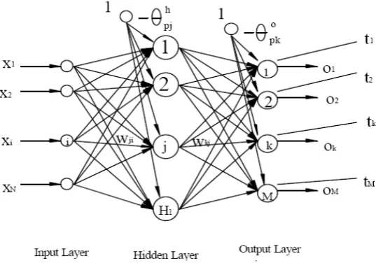
The Back Propagation (BP) neural network is a multilayered, feed forward NN and by far the most extensively utilized due to its well-studied theory. The BP neural network approximates the non-linear relationship between the input and the output by adjusting the weight values internally instead of giving the function expression explicitly. Further, the BP neural network can be generalized for the input that is not included in the training patterns even in the noise-contained environment. Figure 3.3 shows the topology of the BP network that includes only one hidden layer. However, the BPNN can contain more than one hidden layer and the following discussion may be extended to multi-hidden-layer neural networks.
Figure 2.1 Topology of Back Propagation Neural Network In the figure,
x = { x R1R , x R2 R, ….. x RNR } input vector with dimension of N;
o = { o R1R , o R2 R, …...o RMR } output vector of the neural network with dimension of M;
t = { t R1R , tR2 R, …… t RMR } target vector that is the desired output;
wRjiR weight connecting the node j in hidden layer to node i in the input layer.
wRkjR weight connecting node k in out put layer to node j in the last hidden layer.
θRpjR threshold value of pth training pattern, j th node in hidden layer.
θRpk Rthreshold value of pth training pattern, k th node in output layer.
The operation of the BP neural network can be divided into two steps: input feed forward and error back propagation. In the forward step, an input pattern is applied as stimuli to nodes in the input layer, and its effect propagates through the network, layer by layer until an output is produced as the actual response of the network. During this process, the weights of the network are all fixed. The actual output value is then compared to the desired output, and an error signal is computed for each output node. These error signals are transmitted backwards from the output layer to each node in the intermediate layer that contributes directly to the output.
However, each unit in the intermediate layer receives only a portion of the total error signal, based roughly on the relative contribution the unit made to the original output. This process repeats, layer by layer, until each node in the network has received an error signal that describes its relative contribution to the total error. Based on the error signal received, connection weights are then updated by each unit to cause the network to converge toward a state that allows all the training patterns to be encoded.
The back propagation algorithm is used to train the BPNN. This algorithm looks for the minimum of the error function in weight space using the method of gradient descent. The combination of the weights that minimizes the error function is considered to be a solution to the learning problem. The algorithm can be described in the following steps:
2.2 Input feed forward
When the p th training pattern is provided for the input layer, the net input to the j th node in the hidden layer is
netRpjR = Rji xR RiR - wθRpj The output of this node is
oRpjR = fRjR (netRpjR)
similarly, the output of node k in the output layer is netRpkR = RkjR oRpjRw - θRpk
oRpk R= fRkR (netRpkR) = fRkR ( RkjR oRpjwR - θRpkR)
where f j and f k represent the activation functions of the j th node in the hidden layer and the k th node in the output layer. Since the method of gradient descent is used in the algorithm, theactivation function must be continuously derivative. When the binary sigmoid function is used in BPNN, the derivative of this function is f' = f (1- f ) .
2.3 Error calculation
The error between the output of the neural network and desired output can be calculated as Δ RpkR = tRpkR – oRpk
Ep = 0.5 ∑ ΔP
2
PRpkR = 0.5 ∑ ( tRpkR – oRpk R)P
2
2.4 On-line and off-line training process
In the practical application of the BPNN, learning proceeds by many presentations of a prescribed set of training patterns. One complete presentation of the entire training set during the learning process is called an epoch. The learning process is maintained on an epoch-by-epoch basis until the weights of the network stabilize and the average squared error over the entire training set converges to some minimum value.
Two classes of training process can be classified: on-line training process and off-line training process. When the first process is used, the weights of all the layers are updated after a training pattern is provided for the input layer. While for the second process, the weights are updated after all the training patterns are provided for the network. The error calculation in this case is the sum of the error of each training pattern. However, the first process is normally used for training BPNN.
3. PERMISSIBLE STRESSES OF COLD FORMED COMPRESSION
MEMBERS USING BACKPROPAGATION NEURAL NETWORK
The backpropagation neural network will be used to predict the Permissible stress and allowable load of cold-formed steel I-sections with lips. As mentioned before, the training behaviour of a neural network is a trial-and-error process. Therefore, in this chapter, an I-section with lips, of thickness t =
2.5mm is discussed
3.1 COLD-FORMED I-SECTION WITH LIPS OF t = 2.5mm
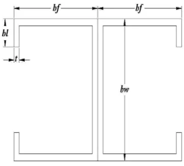
The backpropagation neural network is used to determine the Permissible stress and allowable load of a cold-formed I-section with lips under uniform compression. The dimensions of the I-section with lips are shown in Figure 5.1, where bw is the depth of the web; bf is the width of the flange; bl is the depth of the lip and t is the thickness of the section.
Figure 3.1 Dimension of I- Section with bent lips
As mentioned in the preceding chapter, the configuration and training of neural networks is a trail-and-error process due to such undetermined parameters as the number of nodes in the hidden layer, the learning parameter, and the number of training patterns. Hence, the I-section of 2.5 mmthickness is chosen so as to obtain the experience to configure and train the neural network. The parameters that are used to produce the training data are shown in Table 5.1. Moreover, Young’s Modulus is 250000 N/mmP
2
P
, Effective length is 3500 mm, and Yield stress fy =250 N/mmP
2
P
.
Table 3.1 Input and Output parameters for I-section with bend lips
Input parameters Values
Depth of the web bw (mm) 80, 100, 120, 140, 160, 180, 200 Width of the flange bf (mm) 50, 75, 100, 125
Depth of the lip bl (mm) 10, 15, 20, 25, 30
3.2 Selection of the Training Patterns
The preparation of training data is a matter of considerable importance in training the neural network. However, there are only some guidelines. In this analysis, the Jenkins’ hypercube selection rule, and the modified hypercube rule by Rafiq et al. will be used to select the training patterns.
The hypercube is an imaginary cube on which all the combinations of input are located. The corners of the cube and the value combination on the mid-point of the cube face represent the boundary values of the given input. Further, the point inside the cube should be selected.
Figure 3.2 Data Point for BPNN Training.
Obviously, the point at the centre of the cube should be included. However, this is not enough. Therefore, Jenkins suggested the combination of the input value be taken at random, and the number is about twice that of the total of the corner and mid-side nodes. If the network refuses to train satisfactorily, it is necessary to add more training data.
As far as the inside point in the cube is concerned, Rafiq et al. suggested the centre point of the cube and the mid-point of all sides be selected instead of the random data within the cube. The main scheme of the whole idea is illustrated in Figure 5.2 for three inputs. When it is extended to more input, the cube is imaged as a hypercube.
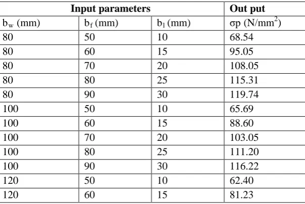
However, according to Euro code 3 part 1.3 (1996), there exist some limits about the section dimension, for instance, bRf R/ t ≤60, 0.2 ≤ bRl R/ bRf R≤ 0.6 and bRw R/ t ≤ 200. Thus, the value of the variable cannot be simply taken from Table 4.1 and combined to form the corner-points, mid face points and centre-points mentioned in the hypercube method. Therefore, the selection of the training pattern considers the limits given in Euro code 3 and the hypercube method is only partially applied. The data details are shown in Table 5.2. And the output is also shown in the table.
Table 3.2 Selection of Training Patterns
Input parameters Out put
bRwR (mm) bRf R(mm) bRl R(mm) σpRR(N/mmP
2
P
)
80 50 10 68.54
80 60 15 95.05
80 70 20 108.05
80 80 25 115.31
80 90 30 119.74
100 50 10 65.69
100 60 15 88.60
100 70 20 103.05
100 80 25 111.20
100 90 30 116.22
120 50 10 62.40
120 60 15 81.23
120 70 20 96.91
120 80 25 105.87
120 90 30 111.48
140 50 10 58.91
140 60 15 73.97
140 70 20 90.64
140 80 25 100.28
140 90 30 106.42
160 50 10 55.37
160 60 15 67.15
160 70 20 84.61
160 80 25 94.82
160 90 30 101.41
180 50 10 52.52
180 60 15 60.86
180 70 20 78.95
180 80 25 89.63
180 90 30 96.60
200 50 10 49.56
200 60 15 55.10
200 70 20 73.69
200 80 25 84.77
200 90 30 92.04
220 50 10 47.15
220 60 15 49.84
220 70 20 68.84
220 80 25 80.23
220 90 30 87.76
The output parameters are Permissible stress and Allowable load. These values are calculated using the MATLAB computer program based on the Analytical method. Figure 5.3 to 5.6 are shows the different relationship between the permissible stress, allowable load, breath of web, breath of flange, breath of lip and ect.
3.3 Selection of the Test Patterns
After training, the neural network can produce the output correctly for the input patterns that are never used in creating and training the neural network. This property of the neural network is called generalization. In this analysis, the generalization of the neural network is evaluated by the test patterns given in Table 5.3. These test patterns are drawn from the same population used to generate the training patterns.
Table 3.3 Selection of Test Patterns
Input parameters Out put
bRwR (mm) bRf bRl R(mm) σpRR(N/mmP
2
P
)
90 55 15 83.76
90 75 20 109.33
90 105 25 121.30
130 55 15 68.03
130 75 20 97.91
130 105 25 112.69
170 55 15 54.61
170 75 20 86.32
170 105 25 103.23
210 55 15 49.16
210 75 20 76.09
210 105 25 94.51
3.4 Training Results
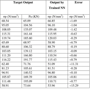
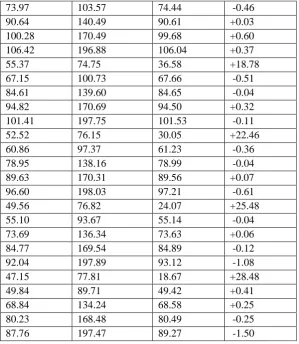
The backpropagation neural network with 3-8-2 nodes in input, hidden and output layers and the selected parameters mentioned above is trained to determine the Permissible stress and Allowable load of the I-section with lip. The output of the trained neural network for the inputs included in the training patterns and the error from the target values are shown in Table 3.4
Table 3.4 Output of the Trained Neural Network for the Training Patterns
Target Output Output by
Trained NN
Error
σpRR(N/mmP
2
P
) Pa (KN) σpRR(N/mmP
2
P
) σpRR(N/mmP
2
P
)
68.54 65.09 66.85 +1.69
95.05 104.56 96.10 -1.04
108.05 135.07 109.48 -1.42
115.31 161.44 115.95 -0.63
119.74 185.60 120.03 -0.29
65.69 68.97 58.90 +6.79
88.60 106.32 88.79 -0.19
103.05 139.12 103.15 -0.09
111.20 166.80 110.54 +0.66
116.22 191.77 115.43 +0.79
62.40 71.76 51.09 +11.31
81.23 105.61 81.51 -0.28
96.91 140.52 96.80 +0.10
105.87 169.39 105.06 +0.81
111.48 195.09 110.71 +0.77
58.91 73.64 53.96 +15.29
73.97 103.57 74.44 -0.46
90.64 140.49 90.61 +0.03
100.28 170.49 99.68 +0.60
106.42 196.88 106.04 +0.37
55.37 74.75 36.58 +18.78
67.15 100.73 67.66 -0.51
84.61 139.60 84.65 -0.04
94.82 170.69 94.50 +0.32
101.41 197.75 101.53 -0.11
52.52 76.15 30.05 +22.46
60.86 97.37 61.23 -0.36
78.95 138.16 78.99 -0.04
89.63 170.31 89.56 +0.07
96.60 198.03 97.21 -0.61
49.56 76.82 24.07 +25.48
55.10 93.67 55.14 -0.04
73.69 136.34 73.63 +0.06
84.77 169.54 84.89 -0.12
92.04 197.89 93.12 -1.08
47.15 77.81 18.67 +28.48
49.84 89.71 49.42 +0.41
68.84 134.24 68.58 +0.25
80.23 168.48 80.49 -0.25
87.76 197.47 89.27 -1.50
3.5 Generalization of Neural Network
The Generalization of the neural network with 3-8-2 node in input, hidden and output layers is monitored by the test patterns. The results are shown in table 5.5
Table 3.5 Generalization of Neural Network for the Test Patterns
Test Patterns
Generalization (Permissible stress and
allowable load)
Generalization Error Dimension of I-section (permissible stress
and allowable load)
bRw bRf bRl σp(N/mmP
2
P
) σp(N/mmP
2
P
) σp(N/mmP
2
P
)
90 55 15 83.76 76.79 +6.97
90 75 20 109.33 105.80 +3.53
90 105 25 121.30 103.07 +18.23
130 55 15 68.03 63.59 +4.47
130 75 20 97.91 100.18 -2.26
130 105 25 112.69 100.95 +11.74
170 55 15 54.61 49.20 +5.40
170 75 20 86.32 93.76 -7.44
170 105 25 103.23 98.70 +4.53
210 55 15 49.16 34.13 +15.02
210 75 20 76.09 86.43 -9.59
210 105 25 94.51 96.28 -1.76
4. CONCLUSION
In the process of training the neural network, the following conclusions can be drawn:
1. The value of the input patterns has a large influence on the training time of the neural network as result of the sigmoid activation function. In this analysis, the input values have been normalized between -1 and 1. The target values of the training patterns have been preprocessed between 0.2 and 0.8, with which the training time has been greatly decreased compared with normalizing the target values between 0 and 1.
2. In this analysis, the convergence of the training becomes faster when the momentum rate is
increased from 0.3 to 0.9, and α = 0.7 has been
network.
3. The number of nodes in the hidden layer is such that the total number of unknowns, i.e. the weights and biases in a neural network, is equal to, or less than the total number of training patterns. The number of nodes is determined by varying the number from 3 or 4 to a maximum value. The final value has been determined by synthesis consideration of the training time, the mapping of the neural network for the training pattern and generalization of the neural network monitored by the test patterns.
4. The neural network, which is trained by the BPNN algorithm showed good generalization and can be used for future research.
REFERENCES
1. Indian Standard 800-1984, code of practice for general construction steel.
2. SP 6 : Part 5 : 1980 Handbook for structural engineers - Cold-formed, light gauge steel structures 3. IS 811 : 1987 Cold formed light gauge structural steel sections
4. Neural Network Toolbox User’s Guide: For Use with MATLAB (1992-1997),
34T
http://www.mathworks.com34T.
5. Kamarthi, S.V., Sanvido, V.E. and Kumara, S.R.T. (1992), Neuroform-Neural Network System for Vertical Formwork Selection. Journal of Computing in Civil Engineering, Vol.6, No.2.
6. Adeli H. and Yeh C. (1989), Perception Learning in Engineering Design. Microcomputers in Civil Engineering Vol.4, No.4, pp. 247-256.
7. Adeli, H. and Park, H.S. (1995), Counterpropagation Neural Networks in Structural Engineering. Journal of Structural Engineering, Vol.121, No.8, pp. 1205-1212.
8. Adeli, H. and Karim, Asim (1997), Neural Network Model for Optimization of Cold-Formed Steel Beams. Journal of Structural Engineering, Vol.123, No.11, pp.1535-1543.
9. Arsian, M.A. and Hajela, P. (1997), Counterpropagation Neural Networks in Decompostion Based Optimal Design. Computers and Structures, Vol.65, No.5, pp. 641-650.
10. AS/NZS 4600 (1996), Australian/New Zealand Standard for Cold-Formed Steel Structures. Sydney: Standards Australia.
11. Bani-Hani, K.and Ghaboussi, J. (1998), Nonlinear Structural Control Using Neural Networks. Journal of Engineering Mechanics, Vol.124, No.3, pp.319-327.
12. Bernard, E.S., Bridge, R.Q. and Hancock, G.J. (1992), Tests of Profiled Steel Decks with VStiffeners. 11th International Specialty Conference on Cold-Formed Steel Structures, St. Louis, Missouri, U.S.A., October 20-21, pp.17-43.
13. Bradford, M.A. (1990), Lateral-Distortional Buckling of Tee-Section Beams. Thin-Walled Structures, Vol.10, No.1, pp.13-30.
14. Carpenter, G.A. and Grossberg, S. (1987), A massively parallel architecture for a selforganizing neural network. Computer Vision, Graphics, and Image Processing, Vol.37, pp. 54-115.