in noncommutative-algebraic cryptography
Boaz Tsaban
Department of Mathematics, Bar-Ilan University, Ramat Gan 52900, Israel [email protected]
http://www.cs.biu.ac.il/~tsaban
Abstract. We introduce the linear centralizer method, and use it to devise a provable polynomial time solution of the Commutator Key Exchange Problem, the computational problem on which, in the passive adversary model, the security of the Anshel–Anshel–Goldfeld 1999Commutator key exchange protocol is based. We also apply this method to the computational problem underlying theCentralizer
key exchange protocol, introduced by Shpilrain and Ushakov in 2006.
This is the first provable polynomial time cryptanalysis of the Commutator key exchange protocol, hitherto the most important key exchange protocol in the realm of noncommutative-algebraic cryp-tography, and the first cryptanalysis (of any kind) of the Centralizer key exchange protocol. Unlike earlier cryptanalyses of the Commutator key exchange protocol, our cryptanalyses cannot be foiled by changing the distributions used in the protocol.
1
Introduction
Since Diffie and Hellman’s 1976 key exchange protocol, few alternative proposals for key exchange protocols (KEPs) resisted cryptanalysis. This, together with the (presently, theo-retical) issue that the Diffie–Hellman and other classic KEPs can be broken in polynomial time by quantum computers, is a strong motivation for searching for substantially different KEPs. Lattice-based KEPs [30] seem to be a viable potential alternative. All classic KEPs as well as the Lattice-based ones are based on commutative algebraic structures.
In 1999, Anshel, Anshel, and Goldfeld [2] (cf. [3]) introduced the Commutator KEP, a general method for constructing KEPs based on noncommutative algebraic structures. Around the same time, Ko, Lee, Cheon, Han, Kang, and Park [20] introduced the Braid Diffie–Hellman KEP, another general method achieving the same goal. The security of both KEPs is based on variations of the Conjugacy Search Problem: Given conjugate elements g, h in a noncommutative group, find x in that group such that x−1gx=h. Both papers [2] and [20] proposed to use the braid group BN, a finitely presented, infinite noncommutative group parameterized by a natural number N, as the platform group.
The introduction of the Commutator KEP and the Braid Diffie–Hellman KEP was fol-lowed by a stream of heuristic attacks (e.g., [15], [16], [23], [14], [10], [25], [11], [12], [17], [24], [26], [28], [29]),1 demonstrating that these protocols, when using the two most simple
distributions on the braid group BN, are insecure. Consequently, a program was set forth, by several independent research groups, to find efficiently sampleable distributions on the braid group that, when used with the above-mentioned protocols, foil all heuristic attacks (e.g., [24], [21], [13], [1]). The abstract of [13] concludes: “Proper choice . . . produces a key exchange scheme which is resistant to all known attacks”. Moreover, a very practical distribution is announced in [36], which foils the strongest known methods for solving the Conjugacy Search Problem in BN.
Most of the mentioned heuristic attacks address the Commutator KEP, and not the Braid Diffie–Hellman KEP. The reason is that in 2003, Cheon and Jun published a provable polynomial time cryptanalysis of the Braid Diffie–Hellman KEP, using a novel representation theoretic method [7]. In their paper, Cheon and Jun stress that their cryptanalysis does not apply to the Commutator KEP and that an extra ingredient is needed. Thus far, no polynomial time attack was found on the Commutator KEP, whose success does not depend on the distributions used in the protocols.
The main result of the present paper is a Las Vegas, provable polynomial time solution of the Commutator Key Exchange Problem (also referred to as the Anshel–Anshel–Goldfeld Problem [27, §15.1.2]), the computational problem underlying the Commutator KEP. This forms a cryptanalysis of the Commutator KEP [2], in the passive adversary model, that succeeds regardless of the distributions used to generate the keys.
The linear centralizer method, developed for our solution of the Commutator Key Ex-change Problem, is applicable to additional computational problems and KEPs in the context of group theory-based cryptography. We present an application of these methods to the Cen-tralizer KEP, introduced by Shpilrain and Ushakov in 2006 [34], to obtain a polynomial time attack. This is the first cryptanalysis, of any kind, of the Centralizer KEP.
We stress that the cryptanalyses presented here, like the Cheon–Jun cryptanalysis, while of polynomial time, are impractical for standard values of N (e.g., N = 100). These results are of theoretic nature. Ignoring logarithmic factors, the complexity of our cryptanalyses is about N17, times a cubic polynomial in the other relevant parameters. Incidentally, though, these cryptanalyses establish the first provable practical attacks in the case where the index N of the braid group BN is small, e.g., when N = 8.
The paper is organized as follows. Section 2 introduces the Commutator KEP and the braid group. In Section 3, we eliminate a technical complexity theoretic obstacle. Section 4 applies a method of Cheon and Jun to reduce our problem to matrix groups over finite fields. Section 5 is the main ingredient of our cryptanalysis, presenting the new method and cryptanalyzing the Commutator KEP in matrix groups. This section is independent of the other sections and readers withour prior knowledge of the braid group may wish to read it first. Section 6 fills a gap in our proof, by applying the Schwartz–Zippel Lemma to obtain a lower bound on the probability that certain random matrices are invertible. Section 7 is a cryptanalysis of the Centralizer KEP, using the methods introduced in the earlier sections. The Braid Diffie–Hellman KEP is introduced in Section 8, where we survey the Cheon–Jun polynomial time cryptanalysis and explain why it does not apply to the Commutator KEP or to the Centralizer KEP. We also describe applications of the new methods to a generalized version of the Braid Diffie–Hellman KEP and to Stickel’s KEP. Some additional discussion is provided in Section 9.
2
The Commutator KEP and the braid group B
NWe will use, throughout, the following basic notation.
Notation 1 For a noncommutative group Gand group elements g, x∈G, gx :=x−1gx, the
conjugate of g by x.
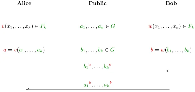
The Commutator KEP [2] is described succinctly in Figure 1.2 In some detail:
1. A noncommutative group Gand elements a1, . . . , ak, b1, . . . , bk ∈Gare publicly given.3 2. Alice and Bob choose free group words in the variables x1, . . . , xk, v(x1, . . . , xk) and
w(x1, . . . , xk), respectively.4
3. Alice substitutes a1, . . . , ak for x1, . . . , xk, to obtain a secret element a=v(a1, . . . , ak)∈ G. Similarly, Bob computes b =w(b1, . . . , bk)∈G.
4. Alice sends the conjugated elements b1a, . . . , bka to Bob, and Bob sends a1b, . . . , akb to Alice.
5. The shared key is the commutator a−1b−1ab. As conjugation is a group isomorphism, we have that
v(a1b, . . . , akb) = v(a1, . . . , ak)b =ab =b−1ab.
Thus, Alice can compute the shared key a−1b−1ab as a−1v(a1b, . . . , akb), using her secret a, v(x1, . . . , xk) and the public elements a1b, . . . , akb. Similarly, Bob computes a−1b−1ab as w(b1a, . . . , bka)−1b.
Alice Public Bob
v(x1, . . . , xk)∈Fk a1, . . . ,ak∈G w(x1, . . . , xk)∈Fk
a=v(a1, . . . ,ak) b1, . . . ,bk∈G b=w(b1, . . . ,bk)
b1a, . . . ,bka //
a1b, . . . ,akb
o
o
a−1b−1ab=a−1v(a1b, . . . ,akb) a−1b−1ab=w(b1a, . . . ,bka)−1
b
Fig. 1.The Commutator KEP
For the platform group G, it is proposed in [2] to use the braid group BN, a group parameterized by a natural number N. The interested reader will find detailed information on BN in almost each of the papers in the bibliography. We quote here the information needed for the present paper.
Let SN be the symmetric group of permutations on N symbols. For our purposes, the braid group BN is a group of elements of the form
(i,p),
2
In our diagrams, green letters indicate publicly known elements, and red ones indicate secret elements, known only to the secret holders. Results of computations involving elements of both colors may be either publicly known, or secret, depending on the context. The colors are not necessary to follow the diagrams.
3 By adding elements, if needed, we assume that the number ofai’s is equal to the number ofbi’s. 4
A free group word in the variablesx1, . . . , xkis a product of the formxi11x
2
i2 · · ·x
m
im , withi1, . . . , im∈ {1, . . . , k}
and1, . . . , m∈ {1,−1}, and with no subproduct of the formxix−1i orx
−1
where i is an integer, and p is a finite (possibly, empty) sequence of elements of SN, that is, p = (p1, . . . , p`) for some ` ≥ 0 and p1, . . . , p` ∈ SN. The sequence p = (p1, . . . , p`) is requested to be left weighted (a property whose definition will not be used here), and p1 must not be the involution p(k) =N −k+ 1.5
Elements of BN are called braids, for they may be identified with braids on N strands. This identification, however, will play no role in the present paper. For “generic” braids (i,(p1, . . . , p`))∈BN,i is negative and|i|is O(`), but this is not always the case. Note that the bitlength of an element (i,(p1, . . . , p`))∈BN is O(log|i|+`NlogN).
Multiplication is defined on BN by an algorithm of complexity O(`2NlogN + log|i|). Inversion is of linear complexity. Explicit implementations are provided, for example, in [6]. For a passive adversary to extract the shared key of the Commutator KEP out of the public information, it suffices to solve the following problem, also referred to as the Anshel– Anshel–Goldfeld Problem [27, §15.1.2].
Problem 2 (Commutator KEP Problem) Let a1, . . . , ak, b1, . . . , bk ∈ BN, each of the
form (i,p) withp of length ≤`. Let a be a product of at most m elements of {a1, . . . , ak}±1,
and let b be a product of at most m elements of {b1, . . . , bk}±1.
Given a1, . . . , ak, b1, . . . , bk, a1b, . . . , abk, ba1, . . . , bak, compute a
−1b−1ab.
Our solution of Problem 2 consists of several ingredients.
3
Reducing the infimum
Theinfimum of a braidb= (i,p) is the integer inf(b) :=i. As the bitlength of bisO(log|i|+ `N logN), an algorithm polynomial in |i|would be at leastexponential in the bitlength. We first remove this obstacle.
In cases where p is the empty sequence, we write (i) instead of (i,p). The properties of
BN include, among others, the following ones.
(a) (i)·(j,p) = (i+j,p) for all integers iand all (j,p)∈BN. In particular, (i) = (1)i for all i.
(b) (2)·(i,p) = (i,p)·(2) for all for all (i,p)∈BN.
Thus, (2j) is a central element ofBN for each integerj. If follows that, for each (i,p)∈BN,
(i,p) = (i−(imod 2))·(imod 2,p).
This way, every braid b ∈ BN decomposes to a unique product c˜b, where c is of the form (2j) (and thus central), and inf(˜b)∈ {0,1}.
Consider the public information in Figure 1. For eachj = 1, . . . , k, decompose as above
aj =cj˜aj,
bj =dj˜bj,
5
For readers familiar with the braid group, we point out that the sequence (i,(p1, . . . , p`)) codes the left normal
form∆ip
with cj, dj central and inf(˜aj),inf(˜bj)∈ {0,1} for all j = 1, . . . , k. Let
˜
a=v(˜a1, . . . ,˜ak); ˜
b=w(˜b1, . . . ,˜bk); c=v(c1, . . . , ck);
d=w(d1, . . . ,d˜k).
As the elements cj, dj are central, we have that
˜
a=v(c−11 a1, . . . , c−1k ak) = v(c−11 , . . . , c −1
k )·v(a1, . . . , ak) = c−1a.
Similarly, ˜b =d−1b. As cand d are central,
ajb = (cja˜j)b =cj˜ajb =cja˜d ˜ b j =cj˜a
˜ b j
for allj = 1, . . . , k. Thus, ˜a˜b
j can be computed for allj. Similarly, ˜bj˜a can be computed. Now,
a−1b−1ab= (c˜a)−1(d˜b)−1(c˜a)(d˜b) = ˜a−1c−1˜b−1d−1c˜ad˜b= ˜a−1˜b−1˜a˜b.
This shows that the Commutator KEP Problem is reducible, in linear time, to the same problem using ˜a1, . . . ,˜ak,˜b1, . . . ,˜bk instead of a1, . . . , ak, b1, . . . , bk. Thus, we may assume that
inf(a1), . . . ,inf(ak),inf(b1), . . . ,inf(bk)∈ {0,1}
to start with. Assume that henceforth.
For a braid x = (i,p), let `(p) be the number of permutations in the sequence p. For integers i, s, let
[i, s] ={x∈BN : i≤inf(x)≤inf(x) +`(x)≤s}.
We use the following basic facts about BN:
1. If x1 ∈[i1, s1] and x2 ∈[i2, s2], then x1x2 ∈[i1+i2, s1+s2]. 2. If x∈[i, s], then x−1 ∈[−s,−i].
Thus, for each x ∈ {a1, . . . , ak, b1, . . . , bk}±1, x±1 ∈ [−`− 1, ` + 1], and therefore, in the notation of our problem, a, b∈[−m(`+ 1), m(`+ 1)]. Thus,
a−1b−1ab∈[−4m(`+ 1),4m(`+ 1)].
Corollary 3 In the Commutator KEP Problem, a−1b−1ab∈[−4m(`+ 1),4m(`+ 1)].
4
Reducing to a matrix group over a finite field
Let n be a natural number. As usual, we denote the algebra of all n×n matrices over a field F by Mn(F), and the group of invertible elements of this algebra by GLn(F). A matrix
group is a subgroup of GLn(F). Afaithful representation of a group Gin GLn(F) is a group isomorphism from Gonto a matrix group H ≤GLn(F). A group is linear if it has a faithful
Bigelow and, independently, Krammer, established in their breakthrough papers [5], [22] that the braid group BN is linear, by proving that the so-called Lawrence–Krammer
repre-sentation
LK : BN −→GL(N
2)(Z [t±1,1
2]), whose dimension is
n:=
N 2
,
is injective.6 The Lawrence–Krammer representation of a braid can be computed in polyno-mial time.7 It is proved implicitly in [22], and explicitly in [7], that this representation is also invertible in (similar) polynomial time. The following result follows from Corollary 1 of [7].
Theorem 4 (Cheon–Jun [7]) Let x∈[i, s] in BN. LetM ≥max(|i|,|s|). Then:
1. The degrees of t in LK(x)∈GLn(Z[t±1,12]) are in {−M,−M + 1, . . . , M}.
2. The rational coefficients c
2d in LK(x) (c integer, d nonnegative integer) satisfy: |c| ≤
2N2M,|d| ≤2N M.
In the notation of Theorem 4, Theorem 2 in Cheon–Jun [7] implies that inversion of LK(x) is of order N6logM multiplications of entries. Ignoring logarithmic factors and thus assuming that each entry multiplication costs N M ·N2M = N3M2, this accumulates to N8M2. This complexity is dominated by the complexity of the linear centralizer step of our cryptanalysis (Section 5).
Let us return to the Commutator KEP Problem 2. By Corollary 3,
K :=a−1b−1ab∈[−4m(`+ 1),4m(`+ 1)].
Let M = 4m(`+ 1). By Theorem 4, we have that
(22N MtM)·LK(K)∈GLn(Z[t]),
the absolute values of the coefficients in this matrix are bounded by 2N2(M+1), and the maximal degree of t in this matrix is bounded by 2M.
Letp be a prime slightly greater than 2N2M
, and f(t) be an irreducible polynomial over
Zp, of degree d slightly larger than 2M. Then
(22N MtM)·LK(K) = (22N MtM)·LK(K) mod (p, f(t))∈GLn(Z[t]/hp, f(t)i),
under the natural identification of {−(p−1)/2, . . . ,(p−1)/2} with {0, . . . , p−1}.
LetF=Z[t]/hp, f(t)i=Z[t±1,12]/hp, f(t)i. F is a finite field of cardinalitypd, whered is the degree off(t). It follows that the complexity of field operations inFis, up to logarithmic factors, of order
d2logp=O(M3N2) = O(m3`3N2).
Thus, the key K can be recovered as follows:
6
Bigelow proved this theorem for the coefficient ringZ[t±1, q±1] with two variables. Krammer proved, in addition,
that one may replaceqby any real number from the interval (0,1).
7 When the infimumiis polynomial in the other parameters, which we proved in Section 3 that we may assume.
1. Apply the composed function LK(x) mod (p, f(t)) to the input of the Commutator KEP Problem, to obtain a version of this problem in GLn(F).
2. Solve the problem there, to obtain LK(K) mod (p, f(t)).
3. Compute (22N MtM)·LK(K) mod (p, f(t)) = (22N MtM)·LK(K). 4. Divide by (22N MtM) to obtain LK(K).
5. Compute K using the Cheon–Jun inversion algorithm.
It remains to devise a polynomial time solution of the Commutator KEP Problem in arbitrary groups of matrices.
5
Linear centralizers
In this section, we solve the Commutator KEP Problem in matrix groups. We first state the problem in a general form. As usual, for a group G and elementsg1, . . . , gk ∈G,hg1, . . . , gki denotes the subgroup of G generated byg1, . . . , gk.
Problem 5 (Commutator KEP Problem) Let G be a group. Leta1, . . . , ak, b1, . . . , bk ∈ G. Let a∈ ha1, . . . , aki, b∈ hb1, . . . , bki.
Given a1, . . . , ak, b1, . . . , bk, a1b, . . . , abk, ba1, . . . , bak, compute a
−1b−1ab. We recall a classic definition.
Definition 6 Let S⊆Mn(F) be a set. The centralizer of S (in Mn(F)) is the set C(S) ={c∈Mn(F) : cs=sc for all s∈S}.
For a1, . . . , ak∈Mn(F), C({a1, . . . , ak}) is also denoted as C(a1, . . . , ak). Basic properties of C(S), that are easy to verify, include:
1. C(S) is a vector subspace (indeed, a matrix subalgebra) of Mn(F). 2. C(C(S))⊇S.
3. C(S) = C(spanS).
4. If S ⊆GLn(F), thenC(S) =C(hSi), where hSi is the subgroup of GLn(F) generated by S.
A key observation is the following one: Let V be a vector subspace of Mn(F), and G ≤ GLn(F) be a matrix group such thatV∩Gis nonempty. It may be computationally infeasible to find an element in V ∩G. However, it is easy to compute a basis forV ∩U for any vector subspaceU of Mn(F). In particular, this is true forU =C(C(G)), that containsG. In certain cases, as the ones below, a “random” element in V ∩C(C(G)) is as good as one in V ∩G.
Following is an algorithm for the Commutator KEP Problem in a matrix group G ≤ GLn(F). The analysis of this algorithm is based on the forthcoming Lemma 9. To this end, we assume that |F|/n ≥ c > 1 for some constant c. In the above section, |F|/n is at least exponential. Fix a finite setS ⊆Fof cardinality greater thancn(the larger the better), that can be sampled efficiently. In the most important case, whereF is a finite field, takeS =F. By random element of a vector subspace V of Mn(F), with a prescribed basis {v1, . . . , vd}, we mean a linear combination
α1v1+· · ·+αkvk
with α1, . . . , αk ∈S uniform, independently distributed.
Algorithm 7
Offline phase:
1. Input: b1, . . . , bk∈G.
2. Execution:
(a) Compute a basis S ={s1, . . . , sd} for C(b1, . . . , bk), by solving the following
homoge-neous system of linear equations in the n2 entries of the unknown matrix x:
b1·x=x·b1
.. .
bk·x=x·bk.
(b) Compute a basis for C(S) = C(C(b1, . . . , bk)), by solving the following homogeneous
system of linear equations in the n2 entries of the unknown matrix x: s1·x=x·s1
.. .
sd·x=x·sd.
3. Output: A basis for C(C(b1, . . . , bk)). Online phase:
1. Input:a1, . . . , ak, b1, . . . , bk, ab1, . . . , abk, b1a, . . . , bak ∈G, wherea∈ ha1, . . . , aki, b∈ hb1, . . . , bki
are unknown. 2. Execution:
(a) Solve the following homogeneous system of linear equations in the n2 entries of the
unknown matrix x:
b1·x=x·b1a
.. .
bk·x=x·bka.
(b) Fix a basis for the solution space, and pick random solutions x until x is invertible. (c) Solve the following homogeneous system of linear equations in the n2 entries of the
unknown matrix y:
a1·y=y·a1b
.. .
ak·y=y·akb,
subject to the linear constraint that y∈C(C(b1, . . . , bk)).
(d) Fix a basis for the solution space, and pick random solutions y until y is invertible. (e) Output: x−1y−1xy.
Letω be the matrix multiplication constant, that is, the minimal such that matrix mul-tiplication isO(nω+o(1)). For our applications, one may takeω = log
27≈2.81. As usual,Las
Theorem 8 Assume that |F|/n≥c > 1 for some constant c, and k ≤n2. Algorithm 7 is a
Las Vegas algorithm for the Commutator KEP Problem, with running time, in units of field operations:
1. Offline phase: O(n2ω+2). 2. Online phase: O(kn2ω).
Proof. We use the notation of Algorithm 7. First, assume that the algorithm terminates. We prove that its output is a−1b−1ab.
x−1y−1xy=x−1y−1(xa−1)ay.
The equations (2)(a) in the online phase of Algorithm 7 assert that bix = bia for all i = 1, . . . , k. Thus, xa−1 ∈ C(b1, . . . , bk). As y ∈ C(C(b1, . . . , bk)), y commutes with xa−1, and therefore so does y−1. Thus,
x−1y−1(xa−1)ay=x−1(xa−1)y−1ay=a−1y−1ay =a−1ay.
By the equations (2)(c) in the online phase of Algorithm 7, aiy = aib for all i = 1, . . . , k. As a ∈ ha1, . . . , aki, we have that ay = ab. Indeed, let a =a1i1 · · ·a
m
im. As conjugation is an
isomorphism,
ay = (a1i1)y· · ·(am
im)
y = (ay i1)
1· · ·(ay im)
m = (ab
i1)
1· · ·(ab im)
m = (a1
i1)
b· · ·(am
im)
b =ab.
Thus,
a−1ay =a−1ab =a−1b−1ab.
Running time, offline phase: (2)(a) These arekn2 equations inn2 variables, and thus the running time is O(k(n2)ω) =O(kn2ω).
(2)(b) AsC(b1, . . . , bk) is a vector subspace of Mn(F), its dimensiondis at mostn2. Thus, the running time of this step is O(n2·n2ω) =O(n2ω+2).
Running time, online phase: (2)(a) As in (2)(a) of the offline phase.
(2)(b) There is an invertible solution to the equations (2)(a), namely: a. Thus, by the Invertibility Lemma 9, the probability that a random solution is not invertible may be assumed arbitrarily close ton/|F| ≤1/c <1. Thus, the expected number of random elements picked until an invertible one was found is constant. To generate one random element, one takes a linear combination of a basis of the solution space. Ifdis the dimension, thend≤n2 and the linear combination takes dn2 ≤ n4 operations. Checking invertibility is faster. The total expected running time of this step is, therefore, O(n4), and n4 ≤n2ω.
(2)(c) Recycling notation, let {s1, . . . , sd} be the basis computed in the offline phase. Thend ≤n2. In the present step, one sets y=t
1s1+· · ·+tdsd, with t1, . . . , tdvariables, and obtains kn2 equations in the d ≤ n2 variables t
1, . . . , td. The complexity is O(kn 2
d d
ω), and
kn2
d d
ω =kn2·dω−1 ≤kn2ω.
(2)(d) Similar to (2)(b).
6
Finding an invertible solution when there is one
The results in the previous section assume that we are able to find, efficiently, an invertible matrix in any subspace of Mn(F) containing an invertible element. This is taken care of by
Lemma 9 (Invertibility Lemma) Let a1, . . . , am ∈Mn(F) be such that span{a1, . . . , am} ∩GLn(F)6=∅.
Let S be a finite subset of F. If α1, . . . , αm are chosen uniformly and independently from S,
then the probability that α1a1+· · ·+αmam is invertible is at least 1− |S|n.
Proof. Let
f(t1, . . . , tm) = det(t1a1+· · ·+tmam)∈F[t1, . . . , tm],
wheret1, . . . , tm are scalar variables. This is a determinant of a matrix whose coefficients are linear in the variables. By the definition of determinant as a sum of products of n elements, f is a polynomial of degree n. As span{a1, . . . , am} ∩GLn(F)6=∅, f is nonzero. Apply the
Schwartz–Zippel Lemma 10.
For the reader’s convenience, we include a proof for the following classic lemma.
Lemma 10 (Schwartz–Zippel) Letf(t1, . . . , tm)∈F[t1, . . . , tm]be a nonzero multivariate
polynomial of degree n. Let S be a finite subset ofF. If α1, . . . , αm are chosen uniformly and
independently from S, then the probability that f(α1, . . . , αm)6= 0 is at least1− |S|n.
Proof. By induction onm. Ifm= 1, thenf is a univariate polynomial of degreen, and thus has at most n roots.
m >1: Write
f(t1, . . . , tm) = f0(t2, . . . , tm) +f1(t2, . . . , tm)t1+f2(t2, . . . , tm)t21+· · ·+fk(t2, . . . , tm)tk1,
with k ≤ n maximal such that fk(t2, . . . , tm) is nonzero. The degree of fk(t2, . . . , tk) is at most m−k. For each choice of α2, . . . , αm ∈ F with fk(α2, . . . , αm) 6= 0, f(t1, α2, . . . , αm) is a univariate polynomial of degree k in the variable t1. By the induction hypothesis (for m = 1), for randomα1 ∈S,f(α1, α2, . . . , αm) is nonzero with probability at least 1−k/|S|. By the induction hypothesis,
Prf(α1, . . . , αm)6= 0
≥ ≥Prfk(α2, . . . , αm)6= 0
·Prf(α1, . . . , αm)= 06 |fk(α2, . . . , αm)6= 0
≥
≥
1−n−k
|S| 1− k |S|
≥1− n |S|.
7
Application to the Centralizer KEP
Definition 11 For a group G and an element g ∈G, the centralizer ofg in G is the set
CG(g) :={h ∈G : gh=hg}.
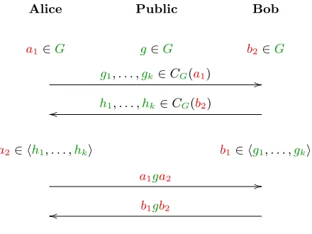
The Centralizer KEP, introduced by Shpilrain and Ushakov in 2006 [34], is described in Figure 2. In this protocol, a1 commutes with b1 anda2 commutes withb2. Consequently, the keys computed by Alice and Bob are identical, and equal to a1b1ga2b2.
Alice Public Bob
a1∈G g∈G b2∈G g1, . . . ,gk∈CG(a1) // h1, . . . ,hk∈CG(b2)
o
o
a2∈ hh1, . . . ,hki b1∈ hg1, . . . ,gki
a1ga2 //
b1gb2
o
o
K=a1b1gb2a2 K=b1a1ga2b2
Fig. 2.The Centralizer KEP
Problem 12 (Centralizer KEP Problem) Assume that g, a1, b2 ∈ BN, g1, . . . , gk ∈ CBN(a1), h1, . . . , hk ∈ CBN(b2), each of the form (i,p) with p of length ≤ `. Let a2 be a product of at most m elements of {h1, . . . , hk}±1, and let b1 be a product of at most m
ele-ments of {g1, . . . , gk}±1.
Given g, g1, . . . , gk, h1, . . . , hk, a1ga2, b1gb2, compute a1b1ga2b2.
7.1 Solving the Centralizer KEP Problem in matrix groups.
For a groupG,Z(G) = CG(G) is the set of all central elements ofG. Consider the Centralizer KEP Problem 12 in G ≤GLn(F) instead of BN. The following variation of this problem is formally harder.8
Problem 13 Let G≤GLn(F). Assume that g, a1, b2 ∈G, g1, . . . , gk ∈CG(a1), h1, . . . , hk ∈ CG(b2), a2 ∈ h{h1, . . . , hk} ∪Z(G)i, and b1 ∈ h{g1, . . . , gk} ∪Z(G)i.
Given g, g1, . . . , gk, h1, . . . , hk, a1ga2, b1gb2, compute a1b1ga2b2.
Following is an algorithm for solving it. As before, for S ⊆ Mn(F), C(S) (without sub-script) is the centralizer of S in the matrix algebra Mn(F).
Algorithm 14
1. Input: g, g1, . . . , gk, h1, . . . , hk, a1ga2, b1gb2 ∈G.
2. Execution:
(a) Compute bases for the subspaces C(g1, . . . , gk), C(C(h1, . . . , hk)) of Mn(F).
(b) Solve
x·g =a1ga2·y
subject to the linear constraints x∈C(g1, . . . , gk), y ∈C(C(h1, . . . , hk)).
(c) Take random linear combinations of the basis of the solution space to obtain solutions
(x, y), until y is invertible.
8
3. Output: x·b1gb2·y−1.
Theorem 15 LetG≤GLn(F). Assume that|F|/n≥c >1for some constantc, andk ≤n2.
Algorithm 14 is a Las Vegas algorithm for Problem 13, with running time, in units of field operations, O(n2ω+2).
Proof. The proof is similar to that of Theorem 8.
First, assume that the algorithm terminates. We prove that its output is a1b1ga2b2. As x∈C(g1, . . . , gk) andb1 ∈ hg1, . . . , gki,xcommutes withb1. Asb2commutes withh1, . . . , hk, b2 ∈C(h1, . . . , hk). Asy∈C(C(h1, . . . , hk)),y commutes withb2, and therefore so does y−1. Thus,
xb1gb2y−1 =b1xgy−1b2.
As xg =a1ga2y,xgy−1 =a1ga2. Thus,
b1xgy−1b2 =b1a1ga2b2 =a1b1ga2b2.
Running time: (2)(a) We are solvingkn2 equations in n2 variables, and then at most n2 equations in n2 variables. This isO(n2ω+2).
(2)(b) We are solving n2 equations in 2n2 variables, which isO(n2ω). (2)(c) Let
H ={(x, y)∈C(g1, . . . , gk)×C(C(h1, . . . , hk)) : x·g =a1ga2·y}
be the solution space, and let (x1, y1), . . . ,(xd, yd) be a basis for H. As H is a subspace of Mn(F)×Mn(F), d ≤ 2n2. Let H2 = {y : (x, y) ∈ H}, the projection of H on the second coordinate. Then
H2 = span{y1, . . . , yd}.
(a1, a−12 )∈H, and thusa −1
2 ∈H2. In particular, there is an invertible element inH2. By the Invertibility Lemma 9, a random linear combination ofy1, . . . , ydis invertible with probability at least 1/c. The total expected running time of this step is, therefore, O(n4), and n4 ≤n2ω.
7.2 Infimum reduction
In Section 3, we explained how each x∈BN can be decomposed (in linear time) as x=cx˜ with c central and inf(x)∈ {0,1}.
We may assume that
inf(g)∈ {0,1}.
Indeed, assume that we have an algorithm solving the problem when inf(g)∈ {0,1}. Write g =cg˜with c central and inf(g)∈ {0,1}. Compute
c−1a1ga2 =a1c−1ga2 =a1˜ga2; c−1b1gb2 =b1c−1gb2 =b1gb˜ 2.
Apply the given algorithm to ˜g, g1, . . . , gk, h1, . . . , hk, a1ga˜ 2, b1gb˜ 2, to obtain a1b1ga˜ 2b2. Mul-tiply by cto obtain a1b1ga2b2.
Next, we may assume that
since when we apply Algorithm 14 in the image of our group in a matrix group, we have in Problem 13 that
h{h1, . . . , hk} ∪Z(G)i=h{h˜1, . . . ,˜hk} ∪Z(G)i; h{g1, . . . , gk} ∪Z(G)i=h{g˜1, . . . ,˜gk} ∪Z(G)i.
As in Section 3, it follows that
a2, b1 ∈[−m(`+ 1), m(`+ 1)].
Let u = a1ga2 and v = b1gb2. Decompose u = cu˜ and v = d˜v with c, d central and inf(˜u),inf(˜v)∈ {0,1}. As g ∈[0, `+ 1] and a1 ∈[inf(a1),inf(a1) +`],
u=a1ga2 ∈[inf(a1),inf(a1) + (m+ 1)(`+ 1) +`],
and thus
a1g(c−1a2) = ˜u∈[0,(m+ 1)(`+ 2)]; c−1a1 = ˜ua−12 g
−1∈
[−(m+ 1)(`+ 1),(m+ 1)(2`+ 3)].
Similarly,
(d−1b1)gb2 = ˜v ∈[0,(m+ 1)(`+ 2)].
Finally,
K0 :=a1(d−1b1)gb2(c−1a2) =a1˜v(c−1a2) = (c−1a1)˜va2 ∈[−(m+ 2)(`+ 1),(m+ 1)(4`+ 6)].
Let M = (m+ 2)(4`+ 6). Continue as in Section 3. By Theorem 4, we have that
(22N MtM)·LK(K0)∈GLn(Z[t]),
the absolute values of the coefficients in this matrix are bounded by 2N2(M+1), and the maximal degree of tin this matrix is bounded by 2M. Letp be a prime slightly greater than 2N2M
, and f(t) be an irreducible polynomial over Zp, of degree d slightly larger than 2M. Then
(22N MtM)·LK(K0) = (22N MtM)·LK(K0) mod (p, f(t))∈GLn(Z[t]/hp, f(t)i),
under the natural identification of {−(p − 1)/2, . . . ,(p − 1)/2} with {0, . . . , p − 1}. Let
F = Z[t]/hp, f(t)i = Z[t±1,12]/hp, f(t)i. F is a finite field of cardinality p
d, where d is the
degree of f(t). It follows that the complexity of field operations in F is, up to logarithmic factors, of order
d2logp=O(M3N2) = O(m3`3N2).
Thus, the key K can be recovered as follows:
1. Apply the composed function LK(x) mod (p, f(t)) to
g, g1, . . . , gk, h1, . . . , hk,u˜=a1g(c−1a2),˜v = (d−1b1)gb2,
to obtain an input to Problem 13.
2. Solve the problem there, to obtain LK(K0) mod (p, f(t)).
3. Compute (22N MtM)·LK(K0) mod (p, f(t)) = (22N MtM)·LK(K0). 4. Divide by (22N MtM) to obtain LK(K0).
8
Further applications
8.1 The Braid Diffie–Hellman KEP
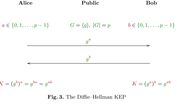
Figure 3 illustrates the well known Diffie–Hellman KEP. Here, G is a cyclic group of prime order, generated by a group element g, and exponentiation denotes ordinary exponentiation.
Alice Public Bob
a∈{0,1, . . . , p−1} G=hgi, |G|=p b∈{0,1, . . . , p−1}
ga //
gb
o
o
K= (gb)a=gba=gab K= (ga)b=gab
Fig. 3.The Diffie–Hellman KEP
Interpreting exponentiation in noncommutative groups as conjugation leads to the Ko– Lee–Cheon–Han–Kang–Park Braid Diffie–Hellman KEP [20]. For subsets A, B of a group G, [A, B] = 1 means that a and b commute, ab = ba, for all a ∈ A, b ∈ B. The Braid Diffie–Hellman KEP is illustrated in Figure 4. Since, in the Braid Diffie–Hellman KEP, the subgroups A and B of G commute element-wise, the keys computed by Alice and Bob are identical. It is proposed in [20] to use Artin’s braid group BN as the platform group G for the Braid Diffie–Hellman KEP, hence the term Braid in the name of this KEP.
Alice Public Bob
a∈A A, B≤G,g∈G,[A,B] = 1 b∈B
ga //
gb
o
o
K= (gb)a=gba K= (ga)b=gab
Fig. 4.The Braid Diffie–Hellman KEP
Problem 16 (Diffie–Hellman Conjugacy Problem) Let A and B be subgroups of G
with [A, B] = 1, and let g ∈G, be given. Given a pair (ga, gb) where a ∈A and b ∈B, find
gab.
The Cheon–Jun atack on the Braid Diffie–Hellman KEP [7] forms a solution to the Diffie– Hellman Conjugacy Problem in the case where Gis the braid groupBN. Their solution can be described, roughly, as follow. Using the methods described in Section 4, the problem is reduced to the case where G ≤ GLn(F), a matrix group over a finite field. Since we are dealing with solutions that are supposed to work for all problem instances, this problem is not harder than that where G = GLn(F), the group of all invertible matices in Mn(F).
However, the latter problem is easy: Assume that B =hb1, . . . , bki ≤G. Solve the system
xga=gx xb1=b1x
.. . xbk=bkx
of (k + 1)n2 linear equations in the n2 entries of the unknown matrix x. There is is an invertible solution to this system, namely, a. Now, any invertible solution ˜a of this system can be used to compute gab: By the first equation,
g˜a= ˜a−1(g˜a) = ˜a−1(˜aga) = ga.
By the remaining equations, ˜a commutes with the generators of B, and consequently with all elements of B. Thus, we can compute
(gb)˜a=gb˜a =g˜ab = (g˜a)b = (ga)b =gab.
This essentially establishes that the Diffie–Hellman Conjugacy Problem in this scenario can be solved in time O(kn2ω).
Comparison with our approach. The reason why the above-mentioned approach of Cheon and Jun is not applicable, as is, to the Commutator KEP or to the Centralizer KEP is that, in either case, there is no prescribed set of generators with which it suffices that the solution commutes: In the Commutator KEP (Figure 1) it is not clear that a has to commute with anything. In the Centralizer KEP (Figure 2), we need a2 to commute with b2, but b2 is secret. The main ingredient in our solution, in both cases, is the replacement of membership in a subgroup with membership in the double centralizer (in the full matrix algebra) of that subgroup, and the observation that the latter is efficiently computable. In other words, instead of adding equations that guarantee that the solution commutes with prescribed elements, we enlarge the set of solutions by moving to the double centralizer, and prove the increase in the set of solutions is not too large.
equations is invertible with overwhelming probability is not proved in [7].9 This gap may be filled using the Invertibility Lemma 9. Third, our approach may be used to push most of the work to the offline phase.
Theorem 17 Assume that |F|/n ≥ c > 1. The Diffie–Hellman Conjugacy Problem for a matrix group G ≤ GLn(F) and B = hb1, . . . , bki is solvable in O(kn2ω) offline time and O(n2ω)online Las Vegas time. More precisely, the running time of the online phase isO(n2ω), plus O(nω) Las Vegas time.
Proof. Offline phase: Compute a basis for the centralizerC(B) in the matrix algebra Mn(F), a solution space of a system of kn2 linear equations in the n2 entries of the variable matrix x. Since C(B) is a subspace of the vector space Mn(F), its dimension d is at most n2. Let c1, . . . , cd be a basis forC(B).
Online phase: Given ga, solve xga = gx subject to x ∈ C(B), a linear system of n2 equations in dscalar variables. Let H be the solution space. Leth1, . . . , hd˜be a basis forH. Then ˜d≤d.
There is an invertible element inH, namely:a. By the Invertibility Lemma 9, ift1, . . . , td˜ are chosen uniformly and independently from a large subset of F, then the matrix ˜a = t1h1+· · ·+td˜hd˜is invertible with probability at least 1/c. Having found such invertible ˜a, compute
g˜a= ˜a−1(g˜a) = ˜a−1(˜aga) = ga.
The running time of the online phase isO(n2ω), plus O(nω) Las Vegas time for the expected constant number of n×n matrix inversions.
Remark 18 In the complexity of the offline phase in Theorem 17, k can be taken to be the minimum among the number of generators of A and the number of generators of B, by exchanging the roles of A and B.
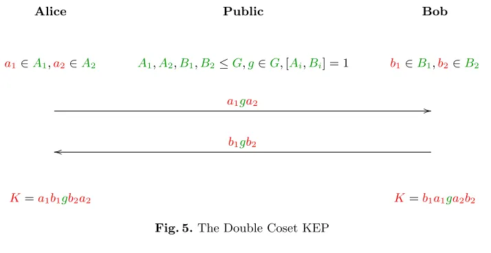
8.2 Double Coset KEPs
In 2001, Cha, Ko, Lee, Han and Cheon [6] proposed a variation of the Braid Diffie–Hellman KEP (Figure 4). For this variation, Cheon and Jun [7] described a convincing variation of their attack. Another variation of this protocol was proposed in 2005, by Shpilrain and Ushakov [33]. Both variations, as well as the Braid Diffie–Hellman KEP, are special cases of the protocol illustrated in Figure 5.
The methods of Theorem 17 extend to the Double Coset KEP. Here too, the restriction to matrix groups is with no loss of generality, and we obtain a polynomial time solution of the underlying problem in the braid group BN.
Theorem 19 Assume that |F|/n ≥ c >1. Let A1, A2, B1 =hb1, . . . , bki, B2 =hb01, . . . , b 0 li ≤ G ≤ GLn(F), with [A1, B1] = [A2, B2] = 1, and g ∈ G. After an offline computation of
complexity O((k +l)n2ω), one can, given a1ga2, b1gb2, compute a1b1ga2b2 in time O(n2ω),
plus O(nω) Las Vegas time. 9
Alice Public Bob
a1∈A1,a2∈A2 A1,A2,B1,B2≤G,g∈G,[Ai,Bi] = 1 b1 ∈B1,b2∈B2
a1ga2 //
b1gb2
o
o
K=a1b1gb2a2 K=b1a1ga2b2
Fig. 5.The Double Coset KEP
Proof. Offline phase: Compute a basis for the centralizersC(B1), C(B2) in the matrix algebra Mn(F), by solving one system ofkn2 linear equations in n2 variables, and another system of ln2 linear equations inn2 variables. Let c1, . . . , cd1 be a basis forC(B1), and c01, . . . , c0d2 be a basis for C(B2). d1, d2 ≤n2.
Online phase: Given a1ga2, solve x(a1ga2) = gy subject to x ∈ C(B1), y ∈ C(B2), a system of n2 equations in d1+d2 ≤2n2 scalar variables. Let H be the solution space,
H ={(x, y)∈C(B1)×C(B2) : x(a1ga2) =gy},
and let (h1, g1), . . . ,(hd, gd) be a basis for H. d≤d1+d2 ≤2n2.
Let H1 = {x : (xy) ∈ H} be the projection of H on the first coordinate. Then {h1, . . . , hd} spans H1. There is an element (x, y) ∈ H with x (and y) invertible, namely: (a−11 , a2). Thus, there is an invertible element in H1. By Lemma 9, if t1, . . . , td are chosen uniformly and independently from a large subset of F, then the matrixx=t1h1+· · ·+tdhd is invertible with probability at least 1/c. Let ˜a2 = t1g1 +· · ·+tdgd. Then (x,a˜2) ∈ H. Compute ˜a1 =x−1. Then
˜
a1g˜a2 =x−1(ga˜2) =x−1(xa1ga2) =a1ga2.
As x∈C(B1), ˜a1 ∈C(B1). Compute
˜
a1b1gb2˜a2 =b1˜a1g˜a2b2 =b1a1ga2b2 =a1b1ga2b2.
An interesting further application is to Stickel’s KEP [35]. This KEP was cryptanalyzed by Shpilrain in [32], describing a heuristic cryptanalysis and supporting it by experimental results. Stickel’s KEP is a special case of the Double Coset KEP, where G = GLn(F), A1 = B1 = h{a} ∪Z(G)i, and A2 = B2 = hbi (a, b public). By Theorem 19, Shpilrain’s cryptanalysis can be turned into a provable Las Vegas polynomial time algorithm, i.e., one supported by a rigorous mathematical proof. In particular, in this way, it is guaranteed that changing the distributions accoring to which the protocol chooses the involved group elements would not defeat the mentioned polynomial time cryptanalysis.
9
Additional comments
our algorithms is
N4ω+6m3`3,
ignoring logarithmic factors. While polynomial, this complexity is practical only for braid groups of small indexN. However, these algorithms constitute the first provable polynomial time cryptanalyzes of the Commutator KEP and of the Centralizer KEP.
The main novelty of our approach lies in the usage of linear centralizers (and double centralizers). However, also the secondary ingredients of our analysis may be of interest. In particular, we have shown that the Invertibility Lemma can be used to turn the Cheon– Jun cryptanalysis of the Braid Diffie–Hellman KEP [7] and the Shpilrain cryptanalysis of Stickel’s KEP [32] into provable Las Vegas algorithms of expected polynomial time, and that the infimum reduction method can be applied to the Cheon–Jun attack to eliminate the exponential dependence on the bitlength of the infimum.
The major challenge is to reduce the degree of N in the polynomial time cryptanaly-ses. By Chinese Remaindering or p-adic lifting methods, it may be possible to reduce the complexity contributed by the field operations. Apparently, this may reduce the power of N by 1. It should be possible to make sure that the Invertibility Lemma is still applicable when these methods are used. Much of the complexity comes from the Lawrence–Krammer representation having dimension quadratic in N. Unfortunately, it is conjectured that there are no faithful representations of BN of smaller dimension. A more careful analysis of the Lawrence–Krammer representation may yield finer estimates. However, it does not seem that any of these directions would make the attacks practical for, say, N = 100.
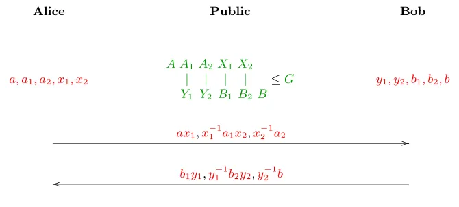
One may wonder whether, from thecomplexity theoreticpoint of view, this paper may end up braid-based cryptography. Our belief is that this is not the case. For example, consider Kurt’s Triple Decomposition KEP [27, 4.2.5], described in Figure 6. In this figure, an edge between two subgroups means that these subgroups commute elementwise. This ensures that the keys computed by Alice and Bob are both equal to ab1a1b2a2b.
Alice Public Bob
a, a1, a2, x1, x2
A A1 A2X1X2
| | | |
Y1 Y2 B1 B2 B
≤G y1, y2, b1, b2, b
ax1,x−11a1x2,x
−1
2 a2 //
b1y1,y
−1
1 b2y2,y
−1
2 b
o
o
K=ab1y1a1y1−1b2y2a2y2−1b K=ax1b1x−11a1x2b2x−21a2b
Fig. 6.The Triple Decomposition KEP
at all. Additional KEPs to which the present methods do not seem to be applicable are introduced by Kalka in [18] and [19]. There are additional types of braid-based schemes (e.g., authentication schemes), that cannot be attacked using the methods presented here. Some examples are reviewed in the monograph [27].
Changing the platform group in any of the studied KEPs is a very interesting option. There are efficiently implementable, infinite groups with no faithful representations as matrix groups (e.g., the braided Thompson group).10
Acknowledgments
I worked on the Commutator KEP, from various other angles, since I was introduced to it at the Hebrew University CS Theory seminar, by Alex Lubotzky [31]. I thank Oleg Bogopol-ski for inviting me, earlier this year (2012), to deliver a minicourse [36] in the conference
Geometric and Combinatorial Group Theory with Applications (D¨usseldorf, Germany, July 25–August 3, 2012). Preparing this minicourse, I discovered the linear centralizer attack. Initially, I addressed the Centralizer KEP (Section 7). When I moved to consider the Com-mutator KEP, Arkadius Kalka pointed out an obstacle mentioned by Shpilrain and Ushakov, that stroke me as solvable by linear centralizers. I am indebted to Kalka for making the right comment at the right time.
I also thank David Garber, Arkadius Kalka, and Eliav Levy, for comments leading to improvements in the presentation of this paper.
References
1. B. An, K. Ko,A family of pseudo-Anosov braids with large conjugacy invariant sets, ArXiv eprint arXiv:1203.2320, 2012.
2. I. Anshel, M. Anshel, D. Goldfeld, An algebraic method for public-key cryptography, Mathematical Research Letters6(1999), 287–291.
3. I. Anshel, M. Anshel, B. Fisher, D. Goldfeld,New Key Agreement Protocols in Braid Group Cryptography, CT-RSA 2001, Lecture Notes in Computer Science2020(2001), 13–27.
4. L´aszl´o Babai, Robert Beals, ´Akos Seress,Polynomial-time theory of matrix groups, ACM STOC 2009, 55–64. 5. S. Bigelow,Braid groups are linear, Journal of the American Mathematical Society14(2001), 471–486. 6. J. Cha, K. Ko, S. Lee, J. Han, J. Cheon,An efficient implementation of braid groups, ASIACRYPT 2001, LNCS
2248(2001), 144–156.
7. J. Cheon, B. Jun,A polynomial time algorithm for the braid Diffie-Hellman conjugacy problem, CRYPTO 2003, Lecture Notes in Computer Science2729(2003), 212–224.
8. P. Dehornoy,Braid-based cryptography, Contemporary Mathematics360(2004), 5–33.
9. D. Garber,Braid group cryptography, in: J. Berrick, F.R. Cohen, E. Hanbury, Y.L. Wong, J. Wu, eds.,Braids: Introductory Lectures on Braids, Configurations and Their Applications, IMS Lecture Notes Series
19, National University of Singapore, 2009, 329–403.
10. D. Garber, S. Kaplan, M. Teicher, B. Tsaban, U. Vishne,Probabilistic solutions of equations in the braid group, Advances in Applied Mathematics35(2005), 323–334.
11. V. Gebhardt, A new approach to the conjugacy problem in Garside groups, Journal of Algebra 292 (2005), 282–302.
12. V. Gebhardt,Conjugacy search in braid groups, Applicable Algebra in Engineering, Communication and Com-puting17(2006), 219–238.
10
As forfinite nonabelian groups, we are pessimistic. For example, finite simple groups tend to be linear of small dimension, by the classification of finite simple groups, and our method would reduce the cryptanalysis to the problem of finding anefficient linear representation of small dimension. There are at present no signs that such representations must be harder to evaluate (or invert) than, say, computing discrete logarithms inZ∗p. Indeed,
13. R. Gilman, A. Miasnikov, A. Miasnikov, A. Ushakov,New developments in Commutator Key Exchange, Proceed-ings of the First International Conference on Symbolic Computation and Cryptography, Beijing, 2008, 146–150. http://www-calfor.lip6.fr/ jcf/Papers/scc08.pdf
14. D. Hofheinz, R. Steinwandt,A practical attack on some braid group based cryptographic primitives, PKC 2003, Lecture Notes in Computer Science2567(2002), 187–198.
15. J. Hughes, A. Tannenbaum,Length-based attacks for certain group based encryption rewriting systems, SECI02: S´ecurit´e de la Communication sur Internet, 2002.
www.ima.umn.edu/preprints/apr2000/1696.pdf
16. J. Hughes,A linear algebraic attack on the AAFG1 braid group cryptosystem, Information Security And Privacy, Lecture Notes in Computer Science2384(2002), 107–141.
17. A. Kalka,Representation attacks on the braid Diffie-Hellman public key encryption, Applicable Algebra in Engi-neering, Communication and Computing17(2006), 257–266.
18. A. Kalka,Representations of braid groups and braid-based cryptography, PhD thesis, Ruhr-Universit¨at Bochum, 2007.
www-brs.ub.ruhr-uni-bochum.de/netahtml/HSS/Diss/KalkaArkadiusG/ 19. A. Kalka,Non-associative public key cryptography, arXiv eprint 1210.8270, 2012.
20. K. Ko, S. Lee, J. Cheon, J. Han, J. Kang, C. Park, New public-key cryptosystem using braid groups, CRYPTO 2000, Lecture Notes in Computer Science1880(2000), 166–183.
21. K. Ko, J. Lee, T. Thomas,Towards generating secure keys for braid cryptography, Design Codes and Cryptography
45(2007), 317–333.
22. D. Krammer,Braid groups are linear, Annals of Mathematics155(2002), 131–156.
23. S. Lee, E. Lee, Potential weaknesses of the commutator key agreement protocol based on braid groups, EURO-CRYPT 2002, Lecture Notes in Computer Science2332(2002), 14–28.
24. S. Maffre,A weak key test for braid-based cryptography, Design Codes and Cryptography39(2006), 347–373. 25. A. Miasnikov, V. Shpilrain, A. Ushakov, A practical attack on some braid group based cryptographic protocols,
CRYPTO 2005, Lecture Notes in Computer Science3621(2005), 86–96.
26. A. Miasnikov, V. Shpilrain, A. Ushakov,Random subgroups of braid groups: an approach to cryptanalysis of a braid group based cryptographic protocol, PKC 2006, Lecture Notes in Computer Science3958(2006), 302–314. 27. A. Miasnikov, V. Shpilrain, A. Ushakov,Non-commutative Cryptography and Complexity of
Group-theoretic Problems, American Mathematical Society Surveys and Monographs177, 2011.
28. A. Miasnikov, A. Ushakov, Length based attack and braid groups: cryptanalysis of Anshel-Anshel-Goldfeld key exchange protocol, PKC 2007, Lecture Notes in Computer Science4450(2007), 76–88.
29. A. Myasnikov, A. Ushakov,Random subgroups and analysis of the length-based and quotient attacks, Journal of Mathematical Cryptology2(2008), 29–61.
30. D. Micciancio, O. Regev,Lattice-based Cryptography, in:Post-quantum Cryptography(D. Bernstein and J. Buchmann, eds.), Springer, 2008.
31. A. Lubotzky,Braid group cryptography, CS Theory Seminar, Hebrew University, March 2001. http://www.cs.huji.ac.il/ theorys/2001/Alex Lubotzky
32. V. Shpilrain,Cryptanalysis of Stickel’s key exchange scheme, in:Computer Science in Russia, Lecture Notes in Computer Science 5010 (2008), 283–288.
33. V. Shpilrain, A. Ushakov,Thompson’s group and public key cryptography, ACNS 2005, Lecture Notes in Computer Science3531(2005), 151–164.
34. V. Shpilrain, A. Ushakov,A new key exchange protocol besed on the decomposition problem, in: L. Gerritzen, D. Goldfeld, M. Kreuzer, G. Rosenberger and V. Shpilrain, eds., Algebraic Methods in Cryptography, Contemporary Mathematics418(2006), 161–167.
35. E. Stickel, A new method for exchanging secret keys, Proceedings of the Third International Conference on Information Technology and Applications (ICITA05), 2005, 426–430.
36. B. Tsaban, The Conjugacy Problem: cryptoanalytic approaches to a problem of Dehn, minicourse, D¨usseldorf University, Germany, July–August 2012.