VICTORIA ! UNIVERSITY
+!
DEPARTMENT OF COMPUTER AND
MATHEMATICAL SCIENCES
Parallel Processing of Aggregate Functions
in the Presence of Data Skew
Kevin H
.
Liu, Yi Jiang and Clement H
.
C
.
Leung
(71 COI\1P 25)
April 1996
(AMS
:
68Pl 5)
TECHNICAL REPORT
VICTORIA UNIVERSITY OF TECHNOLOGY
DEPARTMENT OF COI\1PUTER AND MATHEMATICAL SCIENCES
P 0
BOX 14428
MCMC
MELBOURNE, VICTORIA 8001
AUSTRALIA
TELEPHONE (03) 9688 4492
FACSIMILE (03) 9688 4050
PARALLEL PROCESSING OF AGGREGATE FUNCTIONS
IN
THE PRESENCE OF DATA
SKEW
Kevin H. Liu, Yi Jiang and Clement H. C. Leung
Department of Computer and Mathematical Sciences
Victoria University of Technology, Ballarat Road, Footscray,
PO Box 14428 MMC, Melbourne, Victoria 3000, AUSTRALIA
Email: {kevin, jiang, clement}@matilda.vut.edu.au
Fax: +613-688 4050
ABSTRACT
Parallelising aggregate functions often involves queries of more than one relation, so .
that performance improvement can be achieved in both the intra-operation and inter-operation parallelism levels. Join before aggregation is the conventional way for processing aggregate functions in uni-processor systems and parallel processing of aggregate functions has received little attention. In this paper, the effects of the sequence of aggregation and join operations are identified in a parallel processing environment. Three parallel methods of processing aggregate functions for general queries are presented which mainly differ in their selection of partitioning attribute, i.e JPM partitions on join attribute, APM fragments on group-by attribute, and HPM
adaptively partitions on both join and group-by attribute with a logical hybrid architecture. Their cost models are provided which incorporate the effect of data skew. The performance of these methods are investigated and the results are reported.
1. Introduction
With the increasing complexity of database applications and the advancing inexpensive
multiprocessor technology, parallel query processing has emerged as an efficient way to
improve database performance [DeWi92, Moha94]. The parallelisation of query
processing can be conducted at intra-operation level, inter-operation level or
combination of both. Intra-operation parallelism attempts to, one at a time, distribute
the load of each single relational operation involved in the query to all processors and
performs the operation in parallel; while the inter-operation parallelism aims at
parallelising the operations of the query and allocating them to different processors for
execution [DeWi92].
Parallel processing of major relational operations (e.g. selection, projection and join) has
been studied extensively in recent years [Bell89, Ghan94, Seve90, Kell91, Wolf93a,
Wolf93b]. By contrast, parallel aggregation receives much less attention although it is
critical to the performance of database applications such as decision support, quality
control, and statistical databases. Aggregation may be classified into scalar aggregate
and aggregate fanction [Bitt83, Grae93]. The former refers to the simple aggregation
that produces a single value from one relation such as counting the number of tuples or
summing the quantities of a given attribute; while the latter refers to those that cluster
the tuples of the relation(s) into groups and produce one value for each group. The
queries with aggregate functions often involve more than one relation, and thus require
join operations. The issues on parallel processing scalar aggregate has been studied in
[Shat94] for locally distributed databases. A selectivity estimation is required for their
adaptive methods, and the cost components of the analytical models are provided.
This paper concentrates on the issues of aggregate functions and investigates efficient
parallel processing methods for queries involving aggregations and joins I. Three
methods, namely, join-partition method (JPM), aggregation-partition method (APM)
and hybrid-partition method (HPM), are presented. JPM and APM mainly differ in the
selection of partitioning attribute for distributing workload over the processors and
HPM is an adaptive method based on APM and JPM with a logical hybrid architecture.
Furthermore, all methods take into account the problem of data skew since the skewed
load distribution may affect the query execution time significantly. The performance of
the parallel aggregation methods have been compared under various queries and
different environments with a simulation study, and the ~esults are also presented. In the
next section, we discuss the critical issues on parallelising aggregate functions namely,
the selection of partitioning attribute, the sequence of aggregation and join operation,
and the skewness. The parallel processing methods and their cost models are introduced
in Section 3 followed by a sensitivity analysis in Section 4.
2. Parallelising Aggregate Functions
For simplicity of description and without loss of generality, we consider queries that
involve only one aggregation function and a single join. The example queries given
below arise from a Suppliers-Parts-Projects database. The first query clusters the part
shipment by their city locations and selects the cities with average quantity of shipment
I Hereafter, aggregation means simple aggregation operation (e.g. AVG and SUM on an attribute in one relation) while aggregate function (or aggregation query) consists of aggregation and join operation.
between 500 and 1000. The second query retrieves the project number, name and the
total quantity of shipment for each project.
SUPPLIER {gt, sname, status, city)
PARTS
<J!!l.,
pname, colour, weight, price, city) PROJECT (Ul, jname, city, budget)SHIPMENT (s#, p#, i#, qty)
Query 1: SELECT parts.city, AVG(qty) FROM parts, shipment
WHERE parts.p#=shipment.p# GROUP BY parts.city
HAVING AVG(qty)>500 AND AVG(qty)<lOOO;
Query 2: SELECT project.j#, project.jname, SUM(qty) FROM project, shipment
WHERE project.j#=shipmentj# GROUP BY project.j#, project.name HAVING SUM(qty)>lOOO;
For parallel query processing, we assume a parallel architecture that consists of a host
and a set of working processors as shown in Figure 1. The host accepts queries from
users and distributes each query with required base relations to the processors for
execution. The processors perform the query in parallel with possibly intermediate data
transmission between each other through the network, and finally send the result of the
query to the host.
In the present architecture, an aggregation query is carried out in three phases:
• Data partitioning, the operand relations of the query are partitioned and the
fragments are distributed to each processor;
• Parallel processing, the query is executed in parallel by all processors and
the intermediate results ar~ produced;
• Data consolidation, the final result of the query is obtained by consolidating
the intermediate results from the processors.
HOST
Cross Bar Network
Worker Processor
I I I
Figure 1
2.1 Selection of Partition Attribute
Choosing proper partition attribute is a key issue in the above procedure. Although in
general any attributes of the operand relations may be chosen, two particular attributes,
i.e. join attribute and group-by attribute, are usually considered (e.g. p# and city in the first example query). If the join attribute is chosen, both relations can be partitioned into
N fragments using either range partitioning or hash partitioning strategy, where N is the
number of processors. The cost for parallel join operation can therefore be reduced by a
factor of N2 as compared with a single processor system. However, after join and local
aggregation at each processor, a global aggregation is required at the data consolidation
phase since the local aggregation is performed on a subset of the group-by attribute. In
contrast, if the group-by attribute is used for data partitioning, the relation with the
group-by attribute can be partitioned into N fragments while the other relation needs to
be broadcast to all processors in order to perform the join, leading to a reduction in join
cost by a factor of merely N. Although, in the second method, the join cost is not
reduced as much as in the first method, no global aggregation is required after local join
and aggregation at each processor because the tuples with identical values of the
group-by attribute have been allocated to the same processor. Assuming that there are indexes
on the join attribute and 4 processors, and the execution time is given in terms of the
number of tuples processed in the absence of data skew, Figures 2 and 3 illustrate the
execution time of two types of partitioning strategies on the first example query.
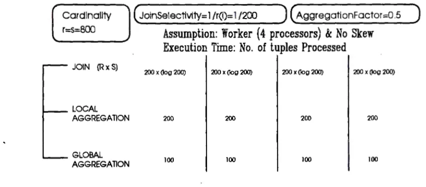
Cardinality (JoinSelectivlty= l /r(I)= 1 /200 ) ( AggregationFactor=0.5
)
r=S=BOO Assumption: Worker (4 processors) & No SkewExecution Time: No. of tuples Processed
JOIN (Rx S)
200 x (log 200) 200 x (log 200) 200 x (log 200) 200 x (log 200)
LOCAL
AGGREGATION 200 200 200 200
GLOBAL
100 100 100 100
AGGREGATION
Figure 2. Join-Partition method
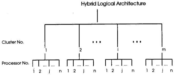
2.2 Sequence of Aggregation and Join Operation
When the join attribute and group-by attribute are the same as shown in the second
example query (i.e. jlf), the selection of partitioning attribute becomes obvious. Instead
of performing join first, the aggregation would be carried out first followed by the join
since the join is more expensive in cost and it would be beneficial to reduce the join
relation sizes by applying aggregation first. Generally, aggregation should always
precede join whenever it is possible with the exception that the size reduction gained
from aggregation is marginal or the join selectivity factor is extremely small. Figure 4
shows that by applying aggregation first, the execution time of the second example
query is much lower than that of join operation first as shown in Figures 2 and 3.
However, aggregation before join may not always be possible, and the semantic issues
on aggregation and join and the conditions under which the aggregation would be
performed before join can be found in [Kim82, Daya87, Bult87, Y an94]. In the
following sections, we assume the more general case where aggregation can not be
executed before join, since earlier aggregation reduces execution time and thus we
process aggregation before join if it is possible.
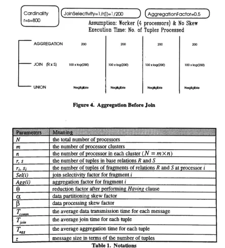
Cardinality r=S=800
JOIN (Rx S)
AGGREGATION
UNION
2.3 Skewness
( JoinSelectivity= l /r(i)= l /200 ) ( AggregationFactor::Cl.5 )
Assumption: Worker (4 processors) & No Skew Execution Time: No. of Tuples Processed
200 x (log 800) 200 x (log 800) 200 x (log 800) 200 x (log 800)
200 200 200 200
Neglgble Neglgble Neglgble Neglgble
·Figure 3. Aggregation-Partition method
Another issue in parallel processing of aggregation queries is the problem of data skew,
and in this context, data skew consists of data partitioning skew and data processing
skew. The data partitioning skew refers to uneven distributing tuples of the operand
relations over the processors and thus results in different processing loads. This is mainly
caused by skewed value distribution in the partitioning attribute as well as improper use
of the partitioning method. The data processing skew, on the other hand, refers to
uneven sizes of the intermediate results generated by the processors. This is caused by
the different selectivity factors of the join/aggregation of the local fragments. Since the
intermediate results of the join operation are processed for aggregation, the data
processing skew may lead to different loads of the processors even when there is no data
partitioning skew. As skewness may reduce the improvement of query response time
gained from parallel processing substantially, it must be considered in parallelising
aggregation queries.
r
Cardinality
f=S=800
(JoinSelectivity= l /r(i)= l /200 ) ( AggregationFactor::0.5 )
Assumption: Worker (4 processors) & No Skew Execution Time: No. of Tuples Processed
AGGREGATION 200 200 200 200
JOIN (Rx S) 100 x iog(200) 100 x log(200) 100 x log(200) 100 x log(200)
UNION Neglgble Neglgble Neglgble Neglgble
Figure 4. Aggregation Before Join
IP.~I1L11tim!miflII1I1I1It1II1IltftIIIIf1@tlttltI1IIltltl@IIlt11@II1Flttm
N the total number of orocessors m the number of orocessor clusters
n the number of processor in each cluster ( N - m X n) r, s the number of tuples in base relations R and S
the number of tuples of fraJmlents of relations R and S at processor i Sel(i) join selectivity factor for fragment i
AgJ.?(i) a1?1?Iegation factor for fraJmlent i
0 reduction factor after performin,!!; Having clause
a. data partitioning skew factor data processing skew factor
~omm the average data transmission time for each message
1Join
the average join time for each tupleT:gg
the average aggregation time for each tuplez
message size in terms of the number of tuplesTable 1. Notations
3. Parallel Processing Methods
We present in this section three parallel processing methods for queries that involve joins
and aggregation functions. The notations used in the description of the methods and in
the subsequent performance evaluation are given in Table I.
3.1 Join Partitioning Method (]PM)
The JPM can be stated as follows. First, the relations R and S are partitioned into N
fragments in terms of join attribute, i.e. the tuples with the same join attribute values in
the two relations fall into a pair of fragments. Each pair of the fragments will be sent to
one processor for execution. Upon receipt of the fragments, in parallel, the processors
perform the join operation and then the local aggregation operation on the fragments
allocated. After that, a global aggregation operation is carried out by. re-distributing the
lqcal aggregation results across the processors such that the result tuples with identical
values of group-by attribute are allocated to the same processors. Then, each processor
performs a N-way merging with the local aggregation results, followed by doing a
restriction operation for the Having clause if exists at local processors. Finally, the host
simply consolidates the partial results from the processors by a union operation, and
produces the query result.
Given the notation early, the execution time for the JPM method can be expressed as
follows
JPM =
~omm
X (max(r;
+s;))
+1j
0in X ( max(r; logs;))+-Z:gg
X (max(r; XS; X Sel(i)))+J:omm X (maxh XS; X Sel{i)x Agg(i)))
+Tagg
x(max(r; Xs;xSel(i)xAgg(i)))x(l+l).
(1)The maximum execution time for each of the components in the above equation varies
with the degree of skewness, and could be far from average execution time. Therefore,
we introduce two skew factors a and ~ to the above cost equation, and a describes the
data partitioning skew while ~ represents the data processing skew. Assume that
a
follows the Zipf distribution where the ith common word in natural language text occurs
with a frequency proportional to i [Knut73, Wolf93b], i.e.
where HN is the Harmonic number and could be approximated to
('Y
+ lnN) [Leun94].Notice that the first element p1 always gives the highest probability and the last element
p N gives the lowest. Considering both operand relations R and S use the same number
of processors and follow the Zipf distribution, the data partitioning skew factor
a
thuscan be represented as
1 1
a=a =a = - = ,
r s HN y+lnN
where 'Y
=
0.57721 known as the Euler Constant and N is the number of processors.The other skew factor ~ for data processing skew is affected by the data partitioning
skew factors in both operand relations since the join/aggregation results rely on the
operand fragments. Therefore, the range of ~ falls in [
ar
xas,
1].
However, the actualvalue of ~ is difficult to estimate because the largest fragments from the two relations
are usually not allocated to the same processor, resulting the
p
much less than theproduct of ar and as. We assume in this paper
p =
(ar x as+ 1)/ 2=
(a
2 + l)! 2 anda detail discussion on skewness can be found in [Liu95, Leun94].
Applying the skew factors to the above cost equation, we also make the following
assumptions and simplifications:
• · Ji
=
1i x si x Sel(i)=
J i.e. in the absence of the skewness,• Agg(i)
=
Agg,• 1)oin
=
Tagg=
Tproc'• data transmission is carried out by message passing with a size
z.
The cost equation (1) can then be re-written below
JPM= i:-{[a(r+s)+ Jx:gg
}z}
[
J
(l
+
1)
x
Jx
Agg] +Tproc ar xlog(as)+i3+ ~[(
r+s 2x(y+lnN)
2
Ji ]
= T
+
2 x J x Aggz
comm y+lnN l+(y+lnN)
r s 2 x y+lnN
+ T log + x J x (1+2 x Agg) .
( )
( )
2
J
'~
y
+In N('Y
+ lnN I+(y
+ lnN)23.2 Aggregation Partitioning Method (APM)
In the APM method, the relation with the group-by attribute, say R, is partitioned into N
fragments in terms of the group-by attribute, i.e. the tuples with identical attribute values
will be allocated to the same processor. The other relation S needs to be broadcast to all
processors in order to perform the binary join. After data distribution, each processor
first conducts the joining one fragment of R with the entire relation S, followed by the
group-by operation and having restriction if exists on the join result. Since the relation R
is partitioned on group-by attribute, the final aggregation result can be simply obtained
by an union of the local aggregation results from the processors, i.e. the step of merging
of the local results used in JPM method is not required. Consequently, the cost of the
AP M can be given by
APM
=
I:omm X (max(rj + s ))+ Tjoin X (max(rj logs))+Tagg X (max(rj X
s
X Sel(j))x (I+ Agg(j)))+i:0mm x (max(rj x s x Sel(j)x Agg(j)x 0 )). (2)
The skew factors
a
and ~ can be added to the above equation in the same way for the JPM method. For the purpose of comparison of the two methods, we assume thatJj = rj xsxSel(j)= J and Agg(j)=
~
Agg. The time of APM method can then beexpressed as
[(
r 2(y+lnN)2 JxAggxeJ 1
J
- T +s+ 2
x
z
- comm
'Y
+ In N 1 + ('Y
+In N) N(
r 2('Y+lnN)2 1
(i
Agg)J+T logs+ 2 x x + - - .
proc
'Y
+ In N 1 + ('Y
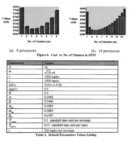
+ In N) N3.3 Hybrid Partitioning Method (HPM)
The HPM method is a combination of the JPM and APM methods. In the HPM, the processors are divided into m clusters each of which has Nim processors as shown in
Figure 5. Based on the proposed logical architecture, the data partitioning phase is
carried out in two steps. First, the relation with group-by attributes is partitioned into
processor clusters in the same way of the APM, i.e. partitioning on the group-by attribute and the other relation is broadcast to the cluster. Second, within each cluster,
the fragments of the first relation and the entire broadcast relation is further partitioned
by the join attributes as the JPM does. Depending on the parameters such as the
cardinality of the relations and the skew factors, a proper value of m will be chosen such
that the minimum query execution time is achieved.
Hybrid Logical Architecture
Cluster No. I I I I I I
I
1 2 m
Processor No.
I
I
_... ...
I__...
I ... 1 ... I I I ... 1 ... I I I ... 1 ... I
I I
... 1 ... 1 2 n 1 2 n 1 2 n 1 2 j nFigure 5. Logical Architecture for HPM
The detail of the HPM method is described below:
Step 1 Partition the relation R on group-by attribute to m clusters, denoted by
r; .
Within each cluster, further partition the fragment r; and the other relation S on
join attribute to n=Nlm processors, denoted by rii and sj. Therefore, the total data
transmission time is given by
~omm
X (max(rij+Si))
where i is in the range of [ 1,m] and j is in the range of [ 1,n].
Step 2 Carry out join at each processor and the maximum processing time is
expressed as
T. ;om . x (max(r .IJ . logs . )) ;
Step 3 Perform local aggregation at each processor with the execution time
Step 4 Redistribute the local aggregation results to the processors within each
cluster by partitioning the results on the group-by attribute. The transmission time
ts given as
T;;omm
X(max(rii
Xsi
XSel(j)x Agg(i)})
Step 5 Merge the local aggregation results within each cluster and this requires. the
time
Step 6 Perform the Having predicate in each cluster with the processing time
Step 7 Transfer the results from the clusters to the host. The time for data·
consolidation in the host is small and thus only data transmission cost is counted,
i.e.
~omm
x
(max(rij x Six Sel(j)x Agg(j)x
e ))
The total execution time of the HPM is the sum of the time of the above steps and can
be given as
+J:0mm X
(max(rii
Xsi
XSel(j)x Agg(j)))
+J:omm
x(max(r;i xsi xSel(j)xAgg(j)xe)).
(3)By applying the same simplification assumptions m the previous methods and
Agg(j)
=.!.
Agg,
(3) is re-written as m. 1 1 l+(y+lnn)2
where J
=
rii
XSi
XSel(J ),
a.n
=
,
a.m
=
,
and ~n=
2 .
y+lnn y+lnm 2(y+lnn)
It can be seen from the above execution time equation that the number of clusters m has
strong influence on the performance of HPM. Figures 6(a) and 6(b) show the changes of
query execution time when increasing the number of clusters in the HPM. It appears that
a value of m =
r
.JNl
approximatelyg~ves
the optimal cost of the query2 although the2Tue approximation can also show the robutne:ss of the adaptive method (HPM).
precise value of m may be worked out by finding the minimum value of the differentiation of the equation (3).
T(Ume 6200 unit) 5700 5200 4700 4200
1 2 3 4 5 6 7 8
No. of Clusters (m)
T(Ume unit) 6000 5500 5000 4500 4000 3500 3000
2500
-1 3 5 7 9 11 13 15 No. of Clusters (m)
(a). 8 processors (b). 16 processors
Figure 6. Cost vs No. of Clusters in HPM
.i!::~ltltttlttittHlV.iiiieiilfrttittftfittltilflfrltJ:ffftllil:tttttttftt:t
N 16
m
.J16=4
r 1000 tuples
s 1000 tuples
Sel(i) 5(N/r)
=
0.08Ae~(i) 0.5
0 0.5
0.2985 0.5446 0.5093
0.5093 0.6297
T;omm
0.1 standard time unit per message 0.01 standard time unit per tuplez
100 tuples per messageTable 2. Default Parameters Values Listing
4. Sensitivity Analysis
The performance of the three parallel processing methods presented may vary with a
number of parameters listed in Table I. In this section, we analysis among them the
effect of the aggregation factor, the join selectivity factor, the degree of skewness (a
and
J3 ),
the relation cardinality, and the ratio of 1;;0mm I Tproc· The default parametervalues are given in Table 2.
•
JPM•
JPM•
APM•
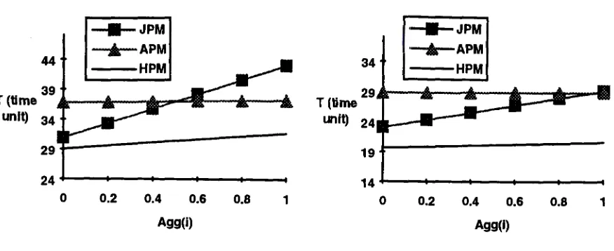
APM144
HPM 34 HPM
T (time 39 T (time 29
unit) 34 unit) 24
29 19
24 14
0 0.2 0.4 0.6 0.8 1 0 0.2 0.4 0.6 0.8 1
Agg(i) Agg(I)
(a). 16 processors (b). 32 processors
Figure 7. Varying Aggregation Factor
4.1 Varying the Aggregation Factor
The aggregation factor ~ is defined by the ratio of result size after aggregation to the
size of the base relation and its impact on three methods is shown in Figure 7. Not
surprisingly, APM is insensitive to aggregation factor. The reasons include little data to
transmit after joining and processing the Having predicate comparing with data
partitioning at beginning and broadcasting relation S, and little data to select with the
group-by condition (Having) as the aggregation factor is reduced by a factor of the
number of processors. Generally, the larger the aggregation factor, the more the running
time is needed as shown in Figure 7(a) with 16 processors. Moreover, increasing the
number of processors will reduce the running time despite data partitioning and
processing skew, and the performance of JPM is better than that of APM except the
aggregation factor is very large as plotted in Figure 7(b) with 32 processors. In both
Figure 7(a) and 7(b), HPM offers the best performance.
94 59
•
JPM•
JPM84
•
APM' 49•
APM74
T (time 64 HPM T (time 39 HPM
1
unit) 54 unit)
29 44
34
19 24
14 9
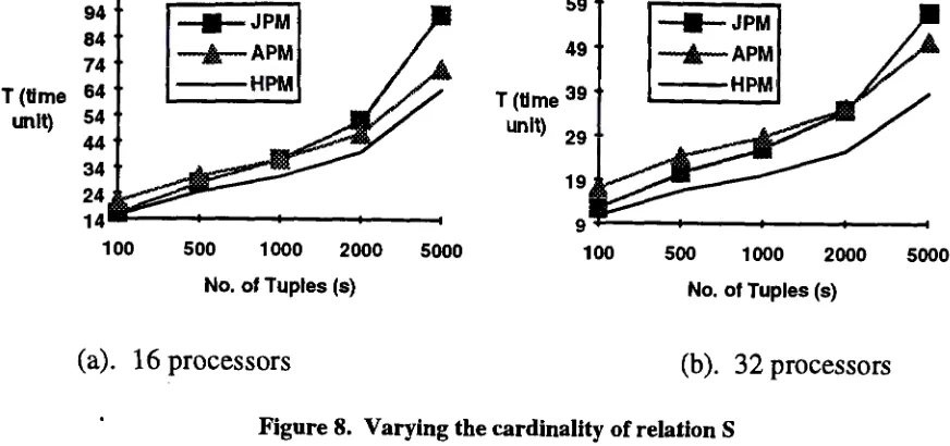
100 500 1000 2000 5000 100 500 1000 2000 5000 No. of Tuples (s) No. of Tuples (s)
(a). 16 processors (b). 32 processors
Figure 8. Varying the cardinality of relation S
4.2 Varying the Relation Cardinality
The cardinality of the operand relations are assumed the same elsewhere in the
sensitivity analysis and their influences on performance are investigated in this
subsection. Figure 8 shows the query execution time when we fix the cardinality of one
relation and increase the cardinality of another relation. JPM appears to be better than
APM only when the varied relation size is small while the HPM again outperforms APM
and JPM in all situations. Comparing 8(a) to 8(b), increasing processors will raise the
cross-over point of JPM and APM.
4.3 Varying the Ratio of T;;omm I Tproc
The ratio of T;;amm I Tprac reflects the characteristic of network used in the parallel
architecture. Primarily, data communication is not a critical issue any more in parallel
database systems comparing with distributed database systems [Alma94]. As we increase
the ratio shown in Figure 9, system performance decreases since we treat Tproc as a
standard time unit and magnify the communication cost, i.e. higher ratio means more
expensive communication. Being a parallel database system, the ratio tends to stay small
and APM is the most sensitive to the communication cost. Nevertheless, HPM will
always perform better than either JPM or APM with improvement on fragmenting
relations within each cluster.
58 61
56 53
51
T (time 48 T (time 46
unit) 43 unit) 41
38 36
31
33 26
28 21
0.1 1 10 100 200 0.1 1 10 100 200
Ratio of Tconvn/Tproc Ratio of Tconvn/Tproc
(a). 16 processors (b). 32 processors
Figure 9. Varying the ratio of Tcomm !Tproc
45
62
•
JPM57 40
•
APM52 35
T (time 47 T (time 30
mlt) 42 mlt)
37 25
32 20
27
22 15
0 2/r 4/r 6/r 8/r 10/r 0 2/r 4/r 6/r 8/r 10/r
Sel(i) Sel(i)
(a). 16 processors (b). 32 processors
Figure 10. Varying the selectivity factor
4.4 Varying the Join Selectivity Factor
The join selectivity factor has significant influence on parallel aggregation processing as
it determines the number of tuples resulting from join intermediately. After that, those
tuples are processed for aggregation and evaluated with the predicates. Eventually, the
qualified tuples are unioned to fonn the query result. Lower selectivity factor involves
less aggregation processing time and transferring time, and thus favours JPM as
displayed in Figure 10. Less processors will reduce the impact of the entire second
relation (both communication and processing) on running time so it favours APM.
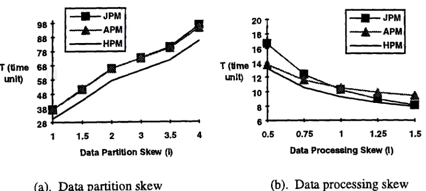
4.5 Varying the Degree of Skewness
Figure 1 l(a) indicates the tendency of the perfonnance when the data processing skew
changes accordingly with the data partitioning skew whereas Figure 11 (b) provides the
comparison when we ignore the data partitioning skew, i.e. a= 1/ N and alter the data
processing skew. The values on the horizontal axis of both figures represent the
expanding skewness factor which then is multiplied by the basic unit given by Zipf
di:;tribution. Unlike the a, the ~ is inversely proportional to data processing skew and
the larger the factor ~ , the less the data processing skew is. We conclude from Figure
11 that either of partitioning skew or processing skew degrades the performance of
parallel processing, HPM outperforms APM and JPM even in the presence of skewness,
and APM is less affected by the skewness compared with JPM .
•
JPM20
•
JPM98
A APM
..
APM18
88 HiPM
16 78
T (time 68 T (time 14
unit) 58 ur'l'lt) 12
48 10
38 8
28 6
1 1.5 2 3 3.5 4 0.5 0.75 1 1.25 1.5 Data Partition Skew (I) Data Processing Skew (I)
(a). Data partition skew (b). Data processing skew
Figure 11. Varying the skewness with 16 processors
84
74
64
T (time 54
unit) 44 34
• JPM
A APM
--HPM
24
14+-~---4--~--~~--...;~
4 8 16 32 64
No. of Processors (N)
135
115
T (time
unit) 75 55
35 15
4 8 16 32 64
No. of Processors (N)
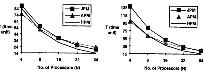
(a). Agg(i)=0.5, Sel(i)=5(Nlr) (b). Agg(i)=0.6, Sel(i)=lO(Nlr)
Figure 12. Varying the number of processors
4.6 Varying the Number of Processors
One of the desired goals of parallel processing is to have linear scale up which can be
achieved when twice as much processors perform twice as large a task in the same time.
When the number of processors is increased, as we expected, the performance is
upgraded in spite of the skewness shown in Figure 12. APM performs extremely well
when the number of processors is small, and it is even better than HPM because the
number of clusters in HPM may not be optimised and less processors make the
communication cost insignificant which favours APM. However, when the database
system scales up, both HPM and JPM performs better than APM.
5. Conclusion
Traditionally, join operation is processed before aggregation operation and relations are
partitioned on join attribute. In this paper, we demonstrate that group-by attribute may
also be chosen as the partition attribute and present three parallel methods for
aggregation queries, JPM, APM, and HPM. These methods differ in the way of
distributing query relations, i.e. partitioning on the join attribute, on the group-by
attribute, or on a combination of both; consequently, they give rise to different query
execution costs. In addition, the problem of data skew has been taken into account in the
proposed methods as it may adversely affect the performance advantage of the parallel
processing. A performance comparison of these methods has been provided under
various circumstances of queries and processors. The results show that when the join
selectivity factor is small and the degree of skewness is low, JPM leads to less cost;
otherwise APM is desirable. Nevertheless, the hybrid method (HPM) is always superior
to the other two methods since the data partitioning is adaptively made on both join
attribute and group-by attribute. In addition, it is found that the partitioning on group-by
attribute method is insensitive to the aggregation factor and thus the method will
simplify algorithm design and implementation.
Reference
[Alma94] Almasi G. S. and A. Gottlieb, "Highly parallel computing", The Benjamin/Cummings
Publishing Company, Inc., 1994
[Bell89] Bell D. A., D. H. 0. Ling, and S. McClean S., "Pragmatic estimation of join sizes
and attribute correlations", Proceedings of 5th IEEE Data Engineering Conference, Los Angeles, 1989
[Bitt83] Bitton D., H. Boral, D. J. DeWitt, and W. K. Wilkinson, "Parallel algorithms for the
execution of relational database operations", ACM Transactions on Database Systems, Vol 8, No.3,
September 1993
[Bult87] Bultzingsloewen G., "Translating and optimizing SQL queries having aggregate",
Proceedings of the 13th International Conference on Very Large Data Bases, Brighton, U.K., 1987
[Daya87] Dayal U., "Of nests and trees: a unified approach to processing queries that contain
nested subqueries, aggregates, and quantitiers", Proceedings of the I 3th International Conference on
Very Large Data Bases, Brighton, U.K., 1987
[DeWi92] DeWitt D.J., J. F. Naughton, D. A. Schneider, and S. Seshadri, "Practical skew
handling in parallel joins", Proceedings of the 8th International Conference on Very Large Data Bases,
Vancouver, British Columbia, Canada 1992
[Ghan94] Ghandeharizadeh S. and D. J. DeWitt, "MAGIC: a multiattribute declustering
mechanism for multiprocessor database machines", IEEE Transactions on Parallel and Distributed
Systems, Vol. 5, No. 5, 1994
[Grae93] Graefe G., "Query evaluation techniques for large databases", ACM Computing
Surveys, Vol.25, No.2, June 1993
[Kell91] Keller A. M. and S. Roy, "Adaptive parallel hash join in main-memory databases",
Proceedings of the I st International Conference on Parallel and Distributed Information Systems, Dec
1991
[~82] Kirn W., "On optimizing an SQL-like nested query", ACM Transactions on Database
Systems, Vol.7, No.3, September 1982
[Knut73] Knuth D. E., "The art of computer programming", Volume 3, Addison-Wesley
Publishing Company, INC., 1973
[Leun94] Leung C. H. C. and K. H. Liu, "Skewness analysis of parallel join execution",
Technical Report, Department of Computer and Mathematical Sciences, Victoria University of
Technology, Melbourne, Victoria, Australia, 1994
[Liu95] Liu K. H., Leung C. H. C., and Y. Jiang, "Analysis and taxonomy of skew in parallel
database systems", High Performance Computing Symposium'95, Montreal, Canada, July 1995, pp
304-315
[Liu96] Liu K. H., Y. Jiang, and C.H.C. Leung, "Query execution in the presence of data
skew in parallel databases", Australian Computer Science Communications, vol 18, no 2, 1996, pp.
157-166
[Moha94] Mohan C., Pirahesh H., Tang W. G., and Y. Wang, "Parallelism in relational database
management systems" IBM Systems Journal, Vol.33, No.2, 1994
[Schn89] Schneider D. A. and D. J. DeWitt, "A perfonnance evaluation of four parallel join
algorithms in a shared-nothing multiprocessor environment", Proceedings of the International
Conference on ACM SIGMOD, New York, U.S.A. 1989
[Seve90] Severance C., Pramanik S., and P. Wolberg, "Distributed linear hashing and parallel
projection in main memory databases", Proceedings of the 16th International Conference on Very Large
Data Bases, Brisbane, Australia 1990
[Shat94] Shatdal A. and J. F. Naughton, "Processing aggregates in parallel database systems",
Computer Sciences Technical Report# 1233, Computer Sciences Department, University of
Wisconsin-Madison, June 1994
[Wolf93a] Wolf J. L., Dias D. M., and P. S. Yu, "A parallel sort-merge join algorithm for
managing data skew", IEEE Transactions On Parallel And Distributed Systems, Vol. 4, No.I, January
1993
[Wolf93b] Wolf J. L., Yu P. S., Turek J. and D. M. Dias, "A parallel hash join algorithm for
managing data skew", IEEE Transactions On Parallel and Distributed Systems, Vol.4, No. 12,
December 1993
[Yan94] Yan W. P. and P. Larson, "Perfonning group-by before join", Proceedings of the
International Conference on Data Engineering, 1994