High-order harmonic generation in a driven two-level atom: Periodic level crossings
and three-step processes
C. Figueira de Morisson Faria
Max Born Institut fu¨r nichtlineare Optik und Kurzzeitspektroskopie, Max Born Strasse 2A, D-12489 Berlin, Germany
I. Rotter
Max Planck Institut fu¨r Physik komplexer Systeme, No¨thnitzer Strasse 38, D-01187 Dresden, Germany 共Received 20 December 2001; published 15 July 2002兲
We investigate high-order harmonic generation in closed systems using the two-level atom as a simplified model. By means of a windowed Fourier transform of the time-dependent dipole acceleration, we extract the main contributions to this process within a cycle of the driving field. We show that the patterns obtained can be understood by establishing a parallel between the two-level atom and the three-step model. In both models, high-order harmonic generation is a consequence of a three-step process, which involves either the continuum and the ground state, or the adiabatic states of the two-level Hamiltonian. The knowledge of this physical mechanism allows us to manipulate the adiabatic states, and consequently the harmonic spectra, by means of a bichromatic driving field. Furthermore, using scaling laws, we establish sharp criteria for the invariance of the physical quantities involved. Consequently, our results can be extended to a broader parameter range, as, for instance, those characteristic of solid-state systems in strong fields.
DOI: 10.1103/PhysRevA.66.013402 PACS number共s兲: 42.50.Hz, 32.80.Rm, 32.80.Qk, 42.65.Ky
I. INTRODUCTION
The generation of high-order harmonics of a strong laser field (I⬃1014 W/cm2) in gaseous samples, where coherent light in the extreme ultraviolet regime is obtained from in-frared input radiation, originated a breakthrough in nonlinear optics. In these systems, composed by atoms or small mol-ecules, high-order harmonic generation 共H.H.G.兲 is a well-understood issue关1兴. These highly nonlinear spectra exhibit very particular features: a frequency region with harmonics of roughly the same intensities, the ‘‘plateau,’’ and a sharp decrease in the harmonic yield at the plateau’s high-energy end, the ‘‘cutoff.’’ Since the early 1990s, not only these fea-tures have been investigated, but also the HHG time profile 关2,3兴, physical mechanisms关4,5兴, and the propagation of the harmonic radiation in gaseous media 关6兴. These studies cul-minated with countless proposals of how to control high har-monics, as diverse as, for instance, polychromatic 关7–9兴 or static关10兴fields, ultrashort pulses 关11兴, or additional poten-tials 关12兴, many of them having even been realized experi-mentally 关13兴.
One of the first models proposed to describe high-order harmonic generation in atoms or diatomic molecules was a two-level atom关4兴. Within this framework, a particularly im-portant paper is关14兴. Therein, it is shown that these harmon-ics are a consequence of the population transfer between the field-dependent states obtained from the diagonalization of the two-level Hamiltonian. This physical mechanism has not been investigated in detail, and there is a very simple reason for this apparent lack of interest: it turned out that an at first sight completely different physical picture is far more suc-cessful in explaining high-order harmonic generation for these systems. This picture, known as ‘‘the three-step model,’’ portraits high-order harmonic generation as a pro-cess in which an electron leaves an atom at an instant t0共the first step兲, propagates in the continuum being accelerated by
the field 共the second step兲, and recombines with the ground state of its parent ion 关5兴at a later time t1, emitting a high-order harmonic photon 共the third step兲. This model has shown that the interplay between a bound state and the con-tinuum, which is not present in a two-level atom, is essential for a correct physical description of high-order harmonic generation. Thus the three-step model has established itself as the paradigm for describing this phenomenon 共see, e.g., 关15兴for a comparison of both models兲.
Until very recently, only gaseous systems were believed to be possible high-order harmonic sources, due to the high intensities involved. However, nowadays, this picture has changed. With the advent of short pulses, there are solid-state materials which can survive the necessary intensity regime, namely 1012⫺1014 W/cm2 关16兴. This has led to theoretical studies on high-order harmonic generation in materials such as thin crystals 关17兴 or carbon nanotubes 关18兴. Another ex-ample of a new and unexpected effect is, for instance, carrier-wave Rabi flopping, which has been recently mea-sured experimentally 关19兴.
Furthermore, apart from this entirely new parameter range, even for considerably lower driving-field intensities, as, for instance, I⬃106 W/cm2, one may in principle extend the frequency of far-infrared radiation (⬃1 GHz) in up to two orders of magnitude by using adequate materials. For instance, for GaAs/AlxGa1⫺xAs wells intersubband
transi-tions of0⬃1 THz may serve this purpose关20兴. Apart from these solid-state materials, HHG involving larger molecules is becoming a problem of interest关21,22兴.
For these complex systems, it is not entirely clear whether bound-to-continuum transitions still yield the most adequate description of high-order harmonic generation. In fact, recent studies have shown that, for aromatic molecules, transitions involving solely bound states are far more important for high-order harmonic generation than the interplay between the ground state and the continuum 关22兴. Thus theoretical
approaches in which the continuum is not taken into account may be possibly used to describe this phenomenon in sys-tems as, for instance, quantum wells 关20,23–26兴. Further-more, descriptions of nonlinear optical processes in solids are widely based on the Hartree-Fock semiconductor Bloch equations. Under special conditions, such as low doping den-sity, equal effective masses in both subbands involved, par-allel subbands, and not too wide wells, these equations are formally identical to those describing the evolution of a two-level atom. Otherwise, collective effects must be taken into account and this analogy is lost关20,24 –26兴.
A common characteristic of all the above-stated systems is their intrincated internal structure, with the presence, as the external parameters are varied, of several level crossings. In particular concerning HHG, the periodic level crossings caused by the temporal dependence of the laser field are very important关14兴. Thus, in order to control the harmonic spec-tra also in this context, one needs to understand the interplay between the population transfer at these crossings and high-order harmonic generation.
Even in the simplest case for which these level crossings occur, namely a two-level atom, it is only clear that most of the population transfer between the field-dressed states takes place at the level crossings. However, this does not necessar-ily mean that the population transfers, within a field cycle, which contribute to the generation of a particular group of harmonics, occur at the level-crossing times. Unanswered questions in this framework concern not only these times, but also how they depend on the external-field parameters, such as its intensity and frequency, and how one can use this information to control the emission spectra of a ‘‘closed,’’ nonionizing system. Another interesting issue concerns the existence of a one-to-one correspondence between the three-step model and the two-level atom. This was proposed in 关14兴due to the different time scales involved in the process, and in关20兴due to a formally identical expression describing population transfers in both models. In these references, however, there is no proof that this correspondence really holds.
The answer to these questions is the main objective of this work. The paper is organized as follows: in Sec. II we briefly discuss the theoretical background for the studies performed in this paper. In the following sections we present our results. In Sec. III, we concentrate on a detailed analysis of the popu-lation transfers and the time profile of harmonic generation for a monochromatic field. Subsequently 共Sec. IV兲, we pro-vide concrete examples of how an additional driving field may alter the periodic level crossings, and consequently the harmonic emission of a closed system. Furthermore, we ad-dress the scaling behavior of the physical quantities involved 共Sec. V兲, establishing sharp criteria for their invariance. Fi-nally, in Sec. VI we close the paper with some concluding remarks.
II. BACKGROUND
A. Two-level atom
The simplest case for which level crossings occur, and a widely used approximation for describing physical systems,
is a two-level atom 关27兴. Within this picture, the time-dependent wave function is given by
兩共t兲典⫽C0共t兲兩0典⫹C1共t兲兩1典, 共1兲
where Cn(t)⫽
具
n兩(t)典
denotes the overlap of the totalwave function with the nth state of an arbitrary basis. The evolution of the system is described by the time-dependent Schro¨dinger equation,
id dt
冉
C0共t兲 C1共t兲
冊
⫽H冉
C0共t兲
C1共t兲
冊
, 共2兲where H is the Hamiltonian matrix, which, in our case, de-scribes an atom in an external laser field. We use atomic units throughout. The basis states兩n
典
are chosen accordingto the problem at hand. We are particularly interested in a basis which yields sharp, well-separated level crossings in the strong-field regime.
A widely used basis are the field-free-states, also known as the ‘‘diabatic basis.’’ In this case, the Hamiltonian is given by
HD⫽
冉
⫺10/2 x10E共t兲 x10E共t兲 10/2
冊
, 共3兲
where10is the transition frequency between the field-free bound states, E(t)⫽E0f (t) is the external field, and x10the dipole matrix element
具
0D兩xˆ兩1D典
, where 兩nD典
denotes the field-free, ‘‘diabatic’’ basis states. This basis is very conve-nient for studying level crossings in the low-intensity laser field regime. For strong laser fields, however, the field-free states are too strongly mixed, such that a more appropriate basis is needed. Such a basis, which will be called by us ‘‘exchanged basis,’’ is obtained applying the unitary transfor-mationUD→E⫽
1
冑
2冉
1 1
⫺1 1
冊
共4兲onto the diabatic basis. The transformation 共4兲 was used in 关14兴 to interchange the diagonal and the nondiagonal terms of the Hamiltonian共3兲. In this case, the exchanged-basis en-ergies ⫾E⫽⫾x10E(t) cross, and the coupling which causes the crossing is effectively given by10/2. The crossings oc-cur within a time interval t0⫺tc⬍t⬍t0⫹tc, where tcis the
time for which the off-diagonal and diagonal terms of the Hamiltonian become equal and t0 is the time for which the field vanishes. For strong enough fields, the times over which the crossings take place are much smaller than the period of the driving field. Thus, to first approximation, one may as-sume that the crossings take place instantaneously at t0. In the following we call t0 ‘‘crossing times.’’
UD→A⫽
冉
cos sin
⫺sin cos
冊
, 共5兲with⫽⫺1/2arctan关2x10E(t)/10兴. This gives
HA⫽UD→AHUD→A
T ⫽
冉
⫺A
0
0 ⫹A
冊
, 共6兲where the field-dressed energies are given by
⫾A⫽⫾1
2
冑
10 2 ⫹关2x10E共t兲兴2. 共7兲
Applying UD→A to the diabatic basis states, one obtains the
field-dressed, ‘‘adiabatic’’ states
兩0
A共
t兲典⫽cos兩0
D
典
⫹sin兩1
D
典
共8兲
and
兩1
A共t兲典⫽⫺sin兩
0
D
典
⫹cos兩1
D
典
, 共9兲whose energies are, respectively,⫺A and⫹A 关28兴. In order to compute the harmonic spectra, one needs the Fourier trans-form of the time-dependent dipole. This quantity is given, in its length and acceleration form, by
x⫽x10关g共t兲cos 2⫹h共t兲sin 2兴 共10兲
and
x¨⫽⫺102x⫹210x10 2
E共t兲关h共t兲cos 2⫺g共t兲sin 2兴, 共11兲
respectively, with g(t)⫽C0*A
(t)C1A(t)⫹C1*A
(t)C0A(t) and h(t)⫽兩C0A(t)兩2⫺兩C1A(t)兩2, where CnA(t)⫽
具
nA(t)兩(t)典
de-notes the projection of the wave function 兩(t)典
onto an adiabatic state. The equations above are the superposition of two distinct terms, namely the crossed terms and the popu-lation difference between the adiabatic states. Since the population difference h(t) roughly ‘‘follows’’ the field, it contributes mainly to the generation of low harmonics, whereas g(t) is expected to be responsible for the high har-monics. This has been confirmed by numerical studies 共not shown兲.An interesting feature is that, in the extreme limit E0
→⬁, the transformation共5兲formally corresponds to Eq.共4兲 and the dipole length共10兲becomes proportional to the popu-lation difference between the adiabatic states. However, one should keep in mind that, only in this limit, the states ob-tained using Eq.共4兲on the field-free states and the adiabatic states are formally equivalent. In general, this is not the case. In the subsequent sections, we work mainly in the adia-batic basis, and refer to crossings of the exchanged-basis energies. For the adiabatic energies, there are avoided cross-ings. The results discussed in this paper have been obtained from the numerical solution of Eq.共2兲in the adiabatic basis, by means of a fourth-order Runge-Kutta method. Unless stated otherwise, the driving field is turned on instanta-neously.
B. Windowed Fourier transform
For both open and closed systems, high-order harmonic generation is always related to abrupt population transfers. Depending on the group of harmonics, they occur at particu-lar times, which give the main contributions to high-order harmonic generation within a field cycle. For an atom in a strong laser field, for instance, these times are well-known and correspond to the return times t1 of an electron which left an atom at a previous time t0. For a closed system, the times t0correspond to the level-crossing times and the times t1 are still an open question to some extent. A very useful method to extract these latter times from the time-dependent dipole is performing a Fourier transform with a temporally restricted window function. For an arbitrary function f (t
⬘
), this transform isF共t,⍀,兲⫽
冕
⫺⬁ ⫹⬁
dt
⬘
f共t⬘
兲W共t,t⬘
,⍀,兲, 共12兲where t,⍀, and denote the time and harmonic frequency at which the window function is centered, and its temporal width, respectively. We consider a Gabor transform, for which the window function is given by
W共t,t
⬘
,⍀,兲⫽exp关⫺共t⫺t⬘
兲2/2兴exp关i⍀t⬘
兴. 共13兲The usual Fourier transformF(⍀), which yields no temporal information, is recovered for →⬁. The temporal width corresponds to a frequency bandwidth ⍀⫽2/. For a tem-poral width smaller than the period T⫽2/ of the driving field, the peaks in the time-resolved spectra 兩F(t,⍀,)兩2 yield the recombination times t1. This method has been ex-tensively used in the literature, in the three-step model framework关3兴.
III. GENERAL PICTURE
We shall now investigate the connection between HHG and the periodic level crossings in detail and draw a general physical picture of the mechanisms involved. The simplest physical situation for which one can do this is a monochro-matic field
E共t兲⫽E0sin共t兲, 共14兲
where E0 and denote the field strength and frequency, respectively. In this case, the time tcis given by the
condi-tion
tc⫽
10 2x10E0
. 共15兲
If the field amplitude E0 is large enough, then tcⰆ1, and
the avoided crossings of the adiabatic states are well-separated. Thus the crossing times t0 are well-defined and there is efficient population transfer at t0. Hence one expects the corresponding spectrum to exhibit a wide plateau and a sharp cutoff.
transfers between the states兩nA(t)
典
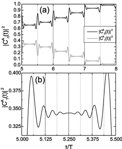
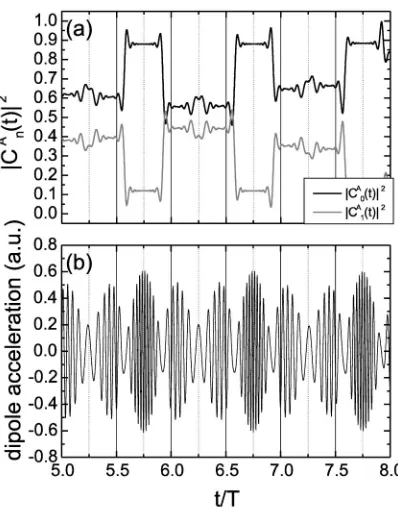
to occur at these times. This is partially confirmed by Fig. 1, where the populations of the adiabatic states are plotted as functions of time. In fact, the pronounced peaks at the times t0 clearly show that most population transfer takes place at these times. There are, however, several smaller peaks, which are symmetric with respect to the times t1 M⫽(2n⫹1)/2 for which the field is maximal. These peaks show that population transfer also occurs at other times, and can be seen in detail in Fig. 1共b兲.The role of these population transfers in HHG can be understood using the Gabor transform of the dipole accelera-tion. The peaks in the Gabor spectra give the main contribu-tions for high-order harmonic generation within a field cycle. For the cutoff harmonic, there is a single peak at t1 M which splits into two for the plateau harmonics. This peak gets further apart as the harmonic frequency decreases, varying from t1 M to the times at the immediate vicinity of the avoided crossings. These results are displayed in Fig. 2.
The physical interpretation of these features is rather simple. At the times the level crossings occur, i.e., at t0 ⫽nT/2, there is a population transfer from the adiabatic state
兩0
A(t)
典
to 兩1
A(t)
典
. The system remains in兩1
A(t)
典
until afurther time t1, decaying back to 兩0
A
(t)
典
and emitting a harmonic of frequency ⍀⫽N⫽⫹A⫺⫺A . The explicit ex-pression relating the time t1 to the harmonic frequency would then bet1⫽arcsin关⫾
冑共
N␥1兲2⫺共␥2兲2兴, 共16兲with ␥1⫽/(2x10E0) and ␥2⫽10/(2x10E0). The physical significance of␥1and␥2will be discussed later in this paper 共Sec. V兲. In order to obtain a harmonic at the maximum possible frequency⍀M共i.e., the cutoff harmonic兲, the
popu-lation transfer between the time-dependent states must occur at the times for which the energy difference⫹A⫺⫺A is maxi-mal, i.e., at t1 M⫽(2n⫹1)/2. As the harmonic energy de-creases, there are two possible times for this population transfer to occur, a shorter and a longer one. The interference between these two possible quantum paths originates the well-structured two-level atom plateau, with sharp harmonic peaks. This process repeats itself every half cycle of the driv-ing field. This picture is supported by the fact that all peaks in the time-resolved spectra satisfy Eq.共16兲and thus can be traced back to population transfers between the adiabatic states. The times given by Eq. 共16兲 for the parameters of Fig. 2, together with the corresponding harmonic energies, are written in Table I.
An analogous picture is observed within the three-step model framework. The cutoff harmonic can only be gener-ated by an electron which returns to its parent ion with maxi-mal kinetic energy. This maximaxi-mal energy corresponds to a particular return time, which appears as a single peak in the Gabor yield. Within the plateau, there are two possible sets of electron trajectories corresponding to the same harmonic energy, such that this single peak splits into two关3兴. In our case, the ‘‘first step’’ would be the population transfer from
兩0
A
(t)
典
to 兩1A
(t)
典
at t0, the ‘‘second step’’ would be the system following 兩1A(t)典
adiabatically in a time interval ⫽t1⫺t0, and the ‘‘third step’’ would be the populationtrans-FIG. 1. Populations兩CnA(t)兩2of the adiabatic states as functions
of time, for transition frequency10⫽0.409 a.u., external field
pa-rameters ⫽0.05 a.u., E0⫽0.6 a.u., and dipole-matrix element x10⫽1.066 a.u. Part共a兲shows this feature for several cycles of the driving field, whereas part共b兲depicts the population of the excited adiabatic state only within half a cycle. The times are given in units of the field cycle T⫽2/. The driving field is turned on linearly within two periods.
FIG. 2. Gabor spectra of the dipole acceleration 关Eq. 共11兲兴as functions of time, for field strength E0⫽1 a.u., field frequency
⫽0.05 a.u., transition frequency10⫽0.409 a.u., and dipole
ma-trix element x10⫽1.066 a.u. The cutoff harmonic lies at ⍀M
⫽43. The time width of the window function was chosen
⫽0.1T. Its center was chosen at the cutoff harmonics, as well as at harmonic energies which roughly correspond to ⍀⫽0.8⍀M, ⍀
⫽0.6⍀M, and ⍀⫽0.4⍀M. All time-resolved spectra have been normalized. The times are given in units of the field cycle T
fer from兩1A(t)
典
to兩0A(t)典
at t1, with subsequent harmonic generation. The corresponding physical picture is illustrated in Fig. 3.Another interesting feature is that the population transfers between the adiabatic states are not strictly periodic within /. Indeed, superposed to them, there are oscillations which occur within much larger time scales, their periods comprising several cycles of the driving field 关29兴. These oscillations are also present in the dipole length and accel-eration as a global enveloping function, whose amplitude, form, and periodicity depend on the field strength E0, the field frequency, and on the dipole matrix element x10 in a nontrivial way. These structures seem not to influence the harmonics globally, but mainly the substructure of the spec-tra and the hyper-Raman lines关30兴.
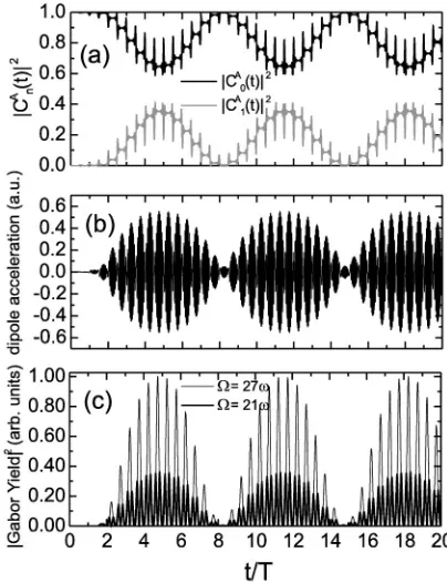
In Fig. 4, we show these enveloping functions for the populations of the adiabatic states关Fig. 4共a兲兴, the dipole
ac-celeration 关Fig. 4共b兲兴, and the Gabor spectra of the plateau and cutoff harmonics 关Fig. 4共c兲兴. One should note that this enveloping function is the same for the Gabor transforms of all groups of harmonics displayed. Furthermore, it does not affect the splitting of the peaks, such that the population transfer times are always given by Eq. 共16兲.
IV. BICHROMATIC DRIVING FIELDS
In this section we consider a bichromatic driving field
E共t兲⫽E01sin共t兲⫹E02sin共nt⫹兲, 共17兲
with two main purposes. First, we wish to confirm the physi-cal picture in which the main contributions to a particular set of harmonics, within a field cycle, occur at the times t1such that the corresponding harmonic frequency is the difference ⫹A⫺
⫺
A between the energies of the adiabatic states. Second,
we are interested in understanding how an additional field can be used to distort the avoided crossings between the adiabatic states in such a way that the harmonic emission can be controlled. In the bichromatic case, depending on the field
TABLE I. Level-crossing times t0, population transfer times t1,
and the corresponding harmonic energy ⍀ for the parameters of Fig. 2. The times are given in units of the period T⫽2/. The harmonic orders, together with the approximate harmonic energies in units of the cutoff frequency⍀M, are given in the remaining two
columns. This pattern repeats itself every half-cycle of the driving field.
t0/T t1/T Harmonic order ⍀/⍀M
0.5 0.25 43 1
0.5 0.14 0.36 35 0.8
0.5 0.09 0.41 25 0.6
0.5 0.05 0.45 17 0.4
FIG. 3. Schematic representation of high-order harmonic gen-eration in a two-level atom. The population transfers at the level crossings occur at the times t0and the main contributions to HHG
occur at the times t1. The times t1 M, t11, and t12correspond to the
generation of the cutoff and plateau harmonics, respectively. The main physical processes are indicated by arrows in the figure, and the corresponding energies can be read in the vertical axis. The adiabatic energies are given in units of the maximal energyMA and the time in units of the field cycle. The field parameters are chosen in such a way that the ratio between the cutoff energy⍀M⫽2M A
and the transition frequency is⍀M/10⫽10.
FIG. 4. Global structures as functions of time, for共a兲the popu-lations兩Cn
A
(t)兩2 of the adiabatic states,共b兲the dipole acceleration x¨(t), and共c兲the Gabor spectra of the cutoff and plateau harmonics. The time width of the window function is ⫽0.1T. The field strength, the field frequency, the transition frequency, and the dipole matrix element were chosen as E0⫽0.6 a.u., ⫽0.05 a.u., 10
⫽0.409 a.u., and x10⫽1.066 a.u., respectively. These parameters
give ␥1⫽0.0391, ␥2⫽0.3197, and a cutoff frequency at ⍀max
parameters, the spectra may have several cutoffs, which are given by the maxima of ⫹A⫺⫺A. Consequently, the main contributions to the generation of the cutoff harmonics take place at the times t1 M for which these maxima occur.
In order to obtain the level-crossing times t0, as well as the times t1 M, one needs the extrema ⫾MA of the field-dressed energies⫾A . For the bichromatic field共17兲they are given by
cos共t兲⫹ncos共nt⫹兲⫽0 共18兲
and
sin共t兲⫹sin共nt⫹兲⫽0, 共19兲
where⫽E02/E01 denotes the field-strength ratio. Equation 共18兲gives the extrema which coincide with those of the field, and therefore t1 M, whereas Eq.共19兲gives those which cor-respond to the avoided crossings, and therefore t0. Depend-ing on the frequency ratio n, the field-strength ratio , and the relative phase , these times, as well as the correspond-ing extrema, can be very different. In this paper we will provide concrete examples for a ⫺2 field, i.e., with n ⫽2, relative phases1⫽0 and2⫽/2, and arbitrary. For these specific parameters, Eqs. 共18兲and共19兲 have a simple form, with analytical solutions.
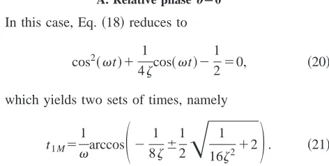
A. Relative phaseÄ0
In this case, Eq.共18兲reduces to
cos2共t兲⫹ 1
4cos共t兲⫺ 1
2⫽0, 共20兲
which yields two sets of times, namely
t1 M⫽ 1
arccos
冉
⫺ 1 8⫾1
2
冑
1
162⫹2
冊
. 共21兲The solutions corresponding to the positive root exist for all field-strength ratios, whereas the remaining solutions are only present for ⬎0.5. Further in this section, it will be shown that the first set gives the absolute maxima of ⫾A , which correspond to the cutoff in the harmonic spectra, whereas the second set yields local maxima at much lower energies.
The expression giving the avoided crossings, on its turn, can be written as
sin共t兲关1⫹2cos共t兲兴⫽0. 共22兲
This equation yields the crossing times t0⫽n/, and t0
⬘
⫽(1/)arccos关⫺1/(2)兴. The crossing times t0 do not de-pend on the field-strength ratio and are the same as in the monochromatic case, whereas the crossing times t0⬘
clearly do. Furthermore, these latter times are only present for ⬎0.5.Figure 5 gives concrete examples of how the adiabatic energies ⫾A depend on time, for different field-strength ra-tios. In contrast to the monochromatic case, ⫾A is not
peri-odic within half a cycle of the driving field. This is not sur-prising, since the periodicity of the field-dressed energies is effectively determined by E2(t) 关cf. Eq. 共7兲兴. For a mono-chromatic field, E2(t)⫽E2(t⫹/) always holds, whereas in the bichromatic case this is only true for odd frequency ratios n. This is clearly not the case addressed in this paper. For the phase ⫽0, one observes that ⫾A(t)⫽⫾A(2/ ⫺t), if both times are taken symmetrically with respect to t0⫽n/. This property already reflects itself in the expres-sions for t0, t1 M, and t0
⬘
derived in this section.Furthermore, one clearly sees that, as predicted in Eq. 共22兲, for ⬍0.5, the second driving wave only distorts the avoided crossings, making them broader at t0⫽(2n ⫹1)/ and sharper at t0⫽2n/. For⫽0.5, the broad crossing starts to split, originating the crossings given at the times t0
⬘
. This splitting also leads to the second set of maxima predicted by Eq.共21兲, which corresponds to a set of harmonics of relatively low frequencies.One must now understand which consequences this effect has on the physical quantities involved. With that purpose, we choose the strengths of both driving waves such thatMA , and therefore the cutoff energy, remains unchanged and is equal to the monochromatic cutoff energy, for variable field-strength ratio. This gives
E01⫽
E0
冑
1⫺2共1⫹2兲, 共23兲 with⫽cos(t1M).The population transfers between the adiabatic states, as functions of time, also exhibit very similar asymmetries to the ones observed in the field-dressed energies. The popula-tion transfers at the broad crossings, for instance, take place at longer time intervals than those at the sharp crossings, making the oscillations in兩Cn
A
(t)兩2 asymmetric with respect to the times t1 M. This asymmetry increases with increasing . An example is provided in Fig. 6共a兲. A similar feature
FIG. 5. Energies of the adiabatic states for a bichromatic field E(t)⫽E01sin(t)⫹E02sin(2t⫹), for ⫽0 and several
field-strength ratios⫽E02/E01. The time t is given in units of the field
occurs for the dipole acceleration. This highly oscillating function exhibits nodes at the level-crossing times. In the monochromatic case, these nodes extend over identical tem-poral regions every half-cycle of the driving field. For bichromatic fields, however, with the distortion of the cross-ings by the second driving wave, this picture changes. There exist narrower and broader nodal regions, corresponding to the narrower and broader crossings, respectively. Thus the oscillations of the dipole acceleration get ‘‘squeezed’’ be-tween the broader nodes. This feature can be seen in Fig. 6共b兲.
The Gabor transform of the dipole acceleration, taken at the cutoff and in the plateau, confirms this picture. In Fig. 7共a兲 there is a clear displacement of the peaks in the time-resolved spectra for the cutoff harmonics, with respect to the monochromatic case, and these peaks occur at the times pre-dicted by Eq. 共21兲. Similarly to the monochromatic case, these peaks split into two in the plateau region, being, how-ever, slightly asymmetric 关Fig. 7共b兲兴. This asymmetry is re-lated to the above-mentioned difference in the shapes of the crossings. Furthermore, for a larger field-strength ratio, the additional times can also be seen for a group of harmonics at the low-energy end of the plateau. The times t0 and t1 M, together with the respective cutoff energies, are given in Table II for the specific parameters considered in this figure.
B. Relative phaseÄÕ2
For this relative phase, Eq. 共18兲has the form
cos共t兲关1⫺2sin共t兲兴⫽0. 共24兲
This equation has two types of solutions: t1 M⫽(n ⫹1/2)/, which do not depend on the field-strength ratio and yield the same maxima as in the monochromatic case, and t1 M
⬘
⫽1/arcsin关1/(4)兴, which clearly depend onand exist only for ⭓0.25. This already hints at a completely different situation as in the previous section, which will nowFIG. 6. Populations 兩Cn A
(t)兩2 of the adiabatic states 关part 共a兲兴 and dipole acceleration关part共b兲兴as functions of time, for a bichro-matic field E(t)⫽E01sin(t)⫹E02sin(2t⫹), with ⫽0,
⫽0.05 a.u., 10⫽0.409 a.u., x10⫽1.066 a.u., and field-strength
ratio⫽E02/E01⫽0.5. The field amplitudes were chosen according
to Eq.共23兲, with E0⫽1 a.u. The time t is given in units of the field
cycle.
FIG. 7. Gabor spectra of the dipole acceleration as functions of time, for a bichromatic field E(t)⫽E01sin(t) ⫹E02sin(2t⫹),
with ⫽0, ⫽0.05 a.u., 10⫽0.409 a.u., x10⫽1.066 a.u., and
several field-strength ratios ⫽E02/E01. The maximal field
strength is kept fixed according to Eq. 共23兲, with E0⫽1 a.u. The
cutoff energy lies at⍀M⫽2M A
⫽43. The temporal width of the window function is ⫽0.1T. In part 共a兲, the window function is centered at the cutoff harmonics, and the field-strength ratio is 0 ⭐⭐0.8. In part共b兲, the center of the window function is taken for different frequencies, and⫽0.8. All curves in the figure have been normalized to their maximum values.
TABLE II. Times for the population transfers between the ex-trema of the adiabatic states, with the approximate order of the corresponding cutoff harmonic, for a bichromatic field given by Eq. 共17兲, with relative phase ⫽0 and several field-strength ratios
⫽E02/E01. The field and two-level atom parameters are the same
as those used in Fig. 7. No entry means that the corresponding maxima do not exist. This pattern repeats itself every cycle T
⫽2/ of the driving field.
⫽0.2 ⫽0.5 ⫽0.8
t0/T t1 M/T ⍀M/ t0/T t1 M/T ⍀M/ t0/T t1 M/T ⍀M/
0 0.20 43 0 0.17 43 0 0.15 43 0.5 0.80 43 0.5 0.83 43 0.36 0.42 9
be discussed in detail. This also holds for the times at which the avoided crossings occur. They must now satisfy
sin2共t兲⫺ 1
2sin共t兲⫺ 1
2⫽0, 共25兲
such that
t0⫽1 arcsin
冉
1 4⫾
1
2
冑
1
42⫹2
冊
, 共26兲all of them depending on . This means that, in contrast to the case ⫽0, one may shift all level-crossing times by changing the relative intensities of the driving waves. The set of crossings given by the positive root in Eq.共26兲exists only for ⭓1, whereas the remaining crossings occur for all.
In Fig. 8 we depict the adiabatic states as functions of time, for several values of, similarly to what was done for ⫽0. This figure illustrates how the relative phase can radi-cally alter the whole physical picture. For⫽/2, already a relatively weak high-frequency wave considerably distorts the avoided level crossings, as well as the maxima of the field-dressed energies. An interesting feature is that the avoided crossings now move with the field-strength ratio. Furthermore, the maximal energies are no longer equal, but, within a field cycle, there are two comparable and different cutoff energies. This can be directly seen by computing the extrema of the energies⫾A, which occur for t1 M.
For field-strength ratio⬍0.25, they give the energies
M1
A ⫽1
2
冑
10 2 ⫹4x10 2共
E01⫺E02兲2 共27兲
and
M2
A ⫽1
2
冑
10 2⫹4x10 2共E
01⫹E02兲2, 共28兲
which correspond to the times t1 M1⫽0.25T mod T, and to t1 M2⫽0.75T mod T, respectively. These times define sym-metry axes for the time-dependence of the adiabatic energies. For ⭓0.25, a further splitting of the set of maxima at t1 M
1 occurs, as predicted in Eq. 共24兲. There exist now two sets of maxima, at the times t1 M
⬘
, whose energies are equal and given byM1
A ⫽1
2
冑
10 2⫹4x10 2 E
01 2 共1⫹8
2兲2
642 . 共29兲
These maxima are symmetric with respect to t1 M1. For these times, the adiabatic energies now exhibit a minimum. This causes, for large , additional avoided crossings 共cf. Fig. 8 for⫽0.8). The population transfers at these times are, how-ever, small, and play only a secondary role in the problem addressed in this paper. For the sake of simplicity, even after the second splitting, we shall refer to the lower-energy set of maxima asM1
A
. The other set of maxima does not split, and the corresponding times t1 M2 remain constant for all. One should note that the adiabatic energies, in the ⫽/2 case, satisfy ⫾A(t)⫽⫾A(T/2⫺t), if both times are chosen sym-metrically with respect to t1 M
1 or t1 M2. This also holds for the population-transfer times derived in this section.
In order to investigate how the distortions in the adiabatic-state energies influence the physical quantities of interest, we shall keep the cutoff energy ⍀M2⫽2M2
A
fixed, and equal to the cutoff energy of the monochromatic case. Thus the field strengths E01and E0 are related by
E01⫽ E0
1⫹. 共30兲
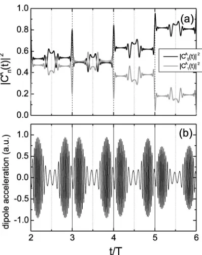
As in the previous section, we can trace all distortions observed in these physical quantities back to those observed in time dependence of ⫾A . For instance, the shifts in the level-crossing times t0predicted by Eq.共26兲are also present in the main population-transfer times for the adiabatic states 关Fig. 9共a兲兴and in the nodes of the dipole acceleration 关Fig. 9共b兲兴. Another effect which is clearly seen in both quantities is the splitting of the maxima near t1 M1⫽0.25T mod T. In-deed, there exist now two sets of maxima which are symmet-ric with respect to these times, for⭓0.25.
We now investigate the Gabor transform of the cutoff and plateau harmonics. In Fig. 10共a兲 we display the time-resolved spectra, centered at the harmonic frequencies ⍀M2
⫽2M2 A
, for different field-strength ratios. The monochro-matic case is also displayed for comparison. As a general feature, for ⫽0, the peaks of the Gabor spectra at t1 M1 ⫽0.25T mod T vanish. This is a direct consequence of the splitting of the extrema of the adiabatic energies caused by the high-frequency wave. Due to this splitting, the energy
FIG. 8. Energies of the adiabatic states for a bichromatic field E(t)⫽E01sin(t)⫹E02sin(2t⫹), for ⫽/2 and several
field-strength ratios⫽E02/E01. The time t is given in units of the field
cycle and the field-dressed energies in units of the maximal energy MA2
. The field parameters were chosen such that⍀M2/10⫽8. The
times t1 Mi are indicated in the figure by the dotted and solid grid
maxima near t1 M1 lie outside the range of the window func-tion and do not contribute to the time-resolved spectra. Fur-thermore, as predicted in Eq.共25兲, the peaks at the maxima t1 M2⫽0.75T mod T do not move in time asis varied.
Taking now the window function 共13兲 centered at ⍀M1
⫽2M1
A 关
Fig. 10共b兲兴, one observes, as expected, a completely different behavior for the peaks near t1 M1⫽0.25T mod T. For ⬍0.25, these peaks are exactly at these times. For ⭓0.25, as expected, they now occur at t1 M
⬘
⫽1/arcsin关1/(4)兴, which vary with the field-strength ratio . Furthermore, this second set of peaks splits for these larger field-strength ratios, such that two sets of peaks which are symmetric with respect to t1 M1 are now present. Other sets of peaks which can be seen in the picture correspond to the upper-plateau return times, which occur for⍀⬍⍀M2andare symmetric with respect to t1 M2⫽0.75T mod T. These peaks come from the splitting of t1 M2, which occurs in this energy range 共cf. Fig. 8兲. The population-transfer times for the specific parameters of this figure, together with the cor-responding harmonic frequencies, are given in Table III.
C. Fourier spectra for the two phases
In the investigations performed so far, our main objective was to understand how an additional driving wave may dis-tort the time dependence of the adiabatic energies and the time profile of harmonic generation. In this section, we ad-dress the question of how these distortions influence the
har-monic spectra. Furthermore, we are interested in extending the cutoff, and, by doing so, guaranteeing that the harmonics in this energy region are strong enough for applicational pur-poses. Clearly, the ideal scenario is to extend the cutoff
en-FIG. 9. Populations 兩Cn A
(t)兩2 of the adiabatic states 关part 共a兲兴 and dipole acceleration关part共b兲兴as functions of time, for a bichro-matic field E(t)⫽E01sin(t)⫹E02sin(2t⫹), with ⫽/2,
⫽0.05 a.u., 10⫽0.409 a.u., x10⫽1.066 a.u., and field-strength
ratio ⫽E02/E01⫽0.8. The time t is given in units of the field
cycle.
FIG. 10. Gabor spectra of the dipole acceleration as a function of time, for a bichromatic field E(t)⫽E01sin(t)⫹E02sin(2t⫹),
with⫽/2,⫽0.05 a.u.,10⫽0.409 a.u., x10⫽1.066 a.u., and
several field-strength ratios ⫽E02/E01. The maximal field
strength is kept fixed according to Eq. 共30兲 and equal to E0
⫽1 a.u. The upper-cutoff energy lies at ⍀M
2⫽43. The
lower-cutoff energy varies with . All cutoff energies are given in Table III, together with the population transfer times t0and t1 M2. In part 共a兲, the window function is centered at the upper-cutoff harmonics (⍀M2⫽2M2
A
), and the field-strength ratio is 0⭐⭐0.8. In part共b兲, the center of the window function is taken at ⍀M1⫽2M1
A
. All curves have been normalized to their maximum values. In part共a兲, the monochromatic case is also displayed for comparison.
TABLE III. Times for the population transfers between the ex-trema of the adiabatic states, with the approximate order of the corresponding cutoff harmonic, for a bichromatic field given by Eq.
共17兲, with relative phase⫽/2 and several field-strength ratios
⫽E02/E01. The field and two-level atom parameters are the same
as those used in Fig. 10. No entry means that the corresponding maxima do not exist. This pattern repeats itself every cycle T
⫽2/ of the driving field. For ⫽0.8, there are additional avoided crossings at 0.25T mod T.
⫽0.2 ⫽0.5 ⫽0.8
t0/T t1 M/T ⍀M/ t0/T t1 M/T ⍀M/ t0/T t1 M/T ⍀M/
0.53 0.75 43 0.56 0.75 43 0.58 0.75 43
0.97 1.25 30 0.94 1.08 23 0.92 1.05 24
0.94 1.42 23 0.92 1.45 24
ergy without any intensity loss in the corresponding har-monic range.
With that purpose, we keep E01 and E02 fixed and com-pare spectra obtained for 1⫽0 and2⫽/2. These results are displayed in Fig. 11. As a global feature, one observes that, for ⫽0, all harmonics behave in a very similar way, with no distinct regions, as for instance a double plateau, in the spectra. This is related to the fact that no splitting of the cutoff energy occurs in this case. The two maxima in ⫾A have the same energy, even though the level-crossing pattern is no longer periodic in T/2. On the other hand, for ⫽/2, there is a clear double-plateau structure. In fact, one can identify a completely different physical behavior for the har-monics in the frequency regions ⍀⬍⍀M1 and ⍀M1⬍⍀
⬍⍀M2. The double-plateau structure is due to the different
cutoff energies which exist in the⫽/2 case.
Another generic feature is that the cutoff energy is ex-tended for ⫽/2. This is expected, since this quantity is given by the maximum energy difference between the adia-batic states. For a field given by Eq. 共17兲, the maximal pos-sible energy is obtained for E(t1 M2)⫽E01⫹E02. This yields the harmonic frequency ⍀M2, discussed in the previous
sec-tion.
There exist, however, nongeneric features, which depend on the absolute field parameters, as, for instance, its strength. Examples of such features are the intensity ratio between the upper and lower parts of the plateau for ⫽/2, and the intensities of the harmonics obtained for⫽/2, compared to those obtained for⫽0. Thus, depending on the absolute parameters used, it is not always possible to extend the cutoff energy without loss of intensity. In order to control HHG in a two-level atom in a more reliable way, a more detailed
study of these features for the particular system in question is necessary.
These nongeneric features are mainly due to the fact that the population transfer at the level crossings is, in general, given by more complicated expressions than in the mono-chromatic case. Indeed, these expressions depend on the shape and width of the crossing, and on the duration of the interaction. These shapes have been studied in 关28,31兴. Fur-thermore, the global structures of the adiabatic-state popula-tions兩CnA(t)兩2have a stronger influence on the spectra in the bichromatic case than for monochromatic driving fields.
Thus the physical picture discussed in Sec. III holds in a more general framework, as, for instance, bichromatic driv-ing fields. Nevertheless, the distortions in the level crossdriv-ings caused by additional fields may have consequences in the quantities involved, including the spectra, which are difficult to predict. This does not mean that control cannot be per-formed at all, but, rather, that it can be done in a restricted context. In fact, one still has a very good predictive power over generic features, as, for instance, the double plateau or the cutoff energies indicated in Fig. 11.
V. SCALING BEHAVIOR
In the results discussed in the previous sections, we have used rather unrealistic frequencies and intensities for the driving fields, for which most physical systems would ionize immediately. This choice of parameters allows us to obtain results with very little numerical effort. In order to extend our computations to more realistic cases, as, for instance, solids, there are two possibilities. Either one slightly in-creases the effort to obtain the necessary precision, or one must find specific combinations of parameters for which the physical quantities involved remain invariant. This second approach has the advantage of providing additional insight into the physics of the problem.
With that purpose, we analyze the scaling behavior of these quantities. We use scaling laws which have been de-rived elsewhere关32兴, in the context of stabilization of atoms in strong laser fields. We concentrate on the question of whether driving fields of much lower frequencies and inten-sities could originate similar spectra, with, for instance, the same number of harmonics, or the same population-transfer times, in units of the field cycle. Therefore our starting point will be the expression
sin共t1兲⫹sin共nt1⫹兲⫽⫾
冑共
N␥1兲2⫺共␥2兲2, 共31兲which relates the harmonic energy to the energy difference of the adiabatic states. This equation gives the population-transfer times. For ⫽0, one has the monochromatic-field case 关Eq. 共16兲兴, and, for ⫽0 and n⫽2, the bichromatic situation discussed in the previous section. Note that the pa-rameters E0, , 10, and x10 appear combined, as ␥1 ⫽/(2x10E0), or ␥2⫽10/(2x10E0). The denominators of these expressions give the Rabi frequencies ⍀R⫽2x10E0, which scale like the energies 关cf. Eqs. 共3兲 and 共6兲 for the two-level Hamiltonian兴. This keeps the Schro¨dinger equation invariant under scale transformations.
FIG. 11. Spectra computed from the dipole acceleration, for the bichromatic field E(t)⫽E01sin(t)⫹E02sin(2t⫹), for ⫽0,
⫽/2, and field strengths E01⫽1.0 a.u. and E02⫽0.2 a.u. The
field is switched on linearly within two cycles. The remaining pa-rameters are⫽0.05 a.u., 10⫽0.409 a.u., x10⫽1.066. The
We now consider the scale transformation
→
⬘
⫽; 10→10⬘
⫽10; ⍀R→⍀R⬘
⫽⍀R,共32兲
where denotes the dilatation factor. The invariance of the Schro¨dinger equation also requires that the time scales as t
→t
⬘
⫽⫺1t, such that Eq.共31兲will remain invariant. This apparently trivial result has far-reaching conse-quences. In fact, it shows that, for any set E0, , 10, and x10, the number of harmonics N in the spectra and the cor-responding population-transfer times t˜1⫽t1/(2), given in terms of field cycles, remain invariant, as long as␥1 and ␥2 are kept constant.Since the unitary transformation共5兲which gives the adia-batic states also depends on E0, ,10, and x10through␥1 and ␥2, it also remains invariant in this case. Thus this in-variance must also hold for the populations of these states, i.e.,兩CnA(t)兩2⫽兩CnA(t
⬘
)兩2.Another quantity of interest is the dipole acceleration. A quick inspection of Eq.共11兲shows that this quantity does not remain invariant under the above-stated transformations. In fact, it scales as x10 multiplied by the square of the energy. The dipole matrix element scales as x10→x10
⬘
⫽⫺1/2x 10. Thus x¨(t)⫽3/2x¨(t
⬘
).The above-stated conclusions are confirmed by Fig. 12. In this figure, we display the same physical quantities as in Fig. 4 for a completely different set of parameters which, how-ever, yield the same␥1 and␥2. The populations兩Cn
A
(t)兩2, in this case 关cf. Fig. 12共a兲兴are, as expected, identical to those depicted in Fig. 4. This is true not only for the oscillations which are periodic in T/2, but also for the global enveloping functions. The scaling with 3/2is also observed for the di-pole acceleration 关Fig. 12共b兲兴. The parameters used in the figure are typical for quantum wells and solid-state systems 关24兴.
Another interesting aspect concerns the resulting har-monic spectra. Even though, in absolute terms, these spectra have different cutoff frequencies and different global inten-sities, for equal ␥1 and ␥2 they have the same shape. Not only the number of harmonics is the same. In addition, all substructure in the spectra looks strikingly similar. These features can be easily understood: the global intensity de-crease is related to the dede-crease in amplitude of the dipole acceleration and the identical shapes are a consequence of the fact that the populations of the adiabatic states, as well as all oscillations present in the dipole acceleration, remain in-variant under the scale transformations discussed here. This is shown in Figs. 13共a兲 and 13共b兲for several dilatation fac-tors . The corresponding field and two-level atom param-eters are given in Table IV.
On the other hand, the behavior of the system can already be altered by small variations in␥1 and␥2. For instance, in Fig. 14 we consider a slightly larger field amplitude than in Fig. 4, which gives different ␥1 and ␥2. In this case, one observes a radically different pattern for the populations
兩CnA(t)兩2 关Fig. 14共a兲兴and the dipole acceleration关Fig. 14共b兲兴.
As a direct consequence, the spectra do not exhibit the same substructure 关Figs. 15共a兲and 15共b兲兴.
VI. CONCLUSIONS
The results discussed in the previous sections lead to the main conclusion that the three-step model and the two-level atom are not completely different physical pictures for de-scribing high-order harmonic generation, as commonly be-lieved. Indeed, in both models, this phenomenon takes place as a result of a three-step process. Hints that a correspon-dence between both physical pictures might exist have been provided in the literature 关14,20兴. We go, however, beyond such studies, giving evidence that a three-step mechanism exists in the two-level atom case and analyzing its features in detail.
In the usual form of the three-step model, there is popu-lation transfer from the atomic ground state to a state in the continuum, i.e., tunneling or multiphoton ionization. The electron then propagates in the continuum within a time in-terval ⫽t1⫺t0, gaining a certain amount of kinetic energy which is converted into harmonic radiation at a time t1, when
FIG. 12. Global structures as functions of time, for共a兲the popu-lations兩Cn
A
(t)兩2of the adiabatic states and共b兲the dipole accelera-tion x¨(t). The field strength, the field frequency, the transiaccelera-tion fre-quency, and the dipole matrix element were chosen as E0⫽6.71
⫻10⫺6 a.u., ⫽2.5⫻10⫺5 a.u., 10⫽2.045⫻10⫺5 a.u., and x10⫽47.673 a.u., respectively. These parameters are typical for
solid-state systems and give␥1⫽0.0391,␥2⫽0.3197, which are the
there is population transfer from the continuum to the ground state, i.e., recombination. In the two-level atom framework, a very similar process takes place: there is population transfer from the field-dressed state兩0A(t)
典
to the state兩1A(t)典
at a time t0 for which an avoided crossing occurs. Subsequently, the system acquires energy from the field within the interval ⫽t1⫺t0, and, at a further time t1, when population transfer from兩1A(t)典
back to兩0A(t)典
takes place, this energy is re-leased in the form of harmonic radiation. Thus the main dif-ference between the three-step model and the two-level atom physical pictures is that in the latter case, the three steps do not involve a continuum state, but a field-dressed bound state.Further similarities are observed in the time profile of high-order harmonic generation. In both cases, the popula-tion transfers which contribute to the generapopula-tion of a particu-lar set of harmonics occur at very specific times. In the usual
three-step model, these times are such that the energy of a particular harmonic must be equal to the sum of the kinetic energy of the electron upon return and the atomic ionization potential. The same line of argumentation holds in the two-level case, but now the harmonic energy must be equal to the energy difference between the adiabatic states at these times. Specifically for monochromatic driving fields, both mod-els share several features. Both in the three-step model and in the two-level atom case there is a single time corresponding to the generation of the cutoff harmonic. In the former model, this time corresponds to the maximal kinetic energy the electron may have, upon return, whereas in the latter model it gives the maximal energy difference between the adiabatic states. Also for both cases, this time splits into two sets of times as the harmonic energy decreases. The interfer-ence between the corresponding population transfers origi-nates the plateau in the high-order harmonic spectra. This pattern repeats itself every half cycle of the driving field. This is a direct consequence of the periodicity of the relevant physical quantities, namely the electron kinetic energy in the three-step model 关33兴 and the adiabatic energies ⫾A in the two-level atom case. All these features are observed as peaks in the Gabor transform of the dipole acceleration. In the three-step model framework, analogous studies have been performed in关3兴.
FIG. 13. Harmonic spectrum for the same parameters as in Fig. 4 (⫽1), compared to those obtained for several field strengths E0,
field frequencies , transition frequencies10, and matrix dipole
elements x10, chosen such that␥1⫽0.0391 and ␥2⫽0.3197, i.e.,
the same as in Fig. 4. These parameters are displayed in Table IV. Part 共a兲 shows the whole spectra, whereas part共b兲 displays both spectra for harmonic order 10⬍N⬍20, such that their substructure can be seen. The field is switched on linearly within two cycles.
TABLE IV. Field and two-level atom parameters, given in atomic units, together with the dilatation factor. All parameters have been chosen such that␥1⫽0.0391 and␥2⫽0.3197.
x10 E0 10
1.066 0.6 0.05 0.409 1
9.535 8.385⫻10⫺4 6.25⫻10⫺4 5.1125⫻10⫺3 1/80 47.673 6.71⫻10⫺6 2.5⫻10⫺5 2.045⫻10⫺4 1/2000
FIG. 14. Global structures as functions of time, for共a兲the popu-lations兩CnA(t)兩2of the adiabatic states and共b兲the dipole
accelera-tion x¨(t). The field strength, the field frequency, the transiaccelera-tion fre-quency, and the dipole matrix element were chosen as E0
⫽0.62 a.u., ⫽0.05 a.u., 10⫽0.409 a.u., and x10⫽1.066 a.u.,
respectively. These parameters are slightly different from the ones in Fig. 4, but give ␥1⫽0.0378, ␥2⫽0.3094. The field is switched
Also for bichromatic driving fields, there are several char-acteristics which are present in both models. A good example is the multiple cutoff structure. Indeed, the harmonic spectra in this case may exhibit several cutoffs, which, depending on the model in question, are given by the maxima of either the electron kinetic energy or of the energy difference between the adiabatic states. The number of these cutoffs, as well as their energies or the corresponding population-transfer times, are determined by the frequency ratio n, the field-strength ratio , and the relative phase . For both the three-step model and the two-level atom, all peaks in the Gabor spectra can be traced back to the population-transfer times. In one or the other case, these population transfers occur either be-tween the adiabatic states共Sec. IV兲, or between the ground-state and the continuum 关8兴.
Similarities between the two models are also observed for the probability that the ‘‘first step,’’ i.e., population transfer, takes place. In the three-step model, this probability, per unit time, is roughly given by the quasi-static tunneling rate P ⬃exp关⫺C/兩E(t0)兩兴 关34兴. A strong field E(t0) at the ioniza-tion time t0 yields strong harmonics at the recombination time t1. This relation is very useful for controlling harmonic spectra, as, for instance, the relative intensities of a double plateau 共see, e.g., 关8,9兴 for concrete examples兲. Within the two-level atom framework and in the monochromatic case, to first approximation, the field-dependent terms of the
two-level Hamiltonian can be linearized at the crossings 关14兴. Thus the population transfer between the exchanged states can be computed by means of the Landau-Zener model 关28,35兴. This probability is approximately given by P ⬃exp关⫺C
⬘
/(2x10E0)兴, such that the Rabi frequency, in the two-level atom, plays a similar role as E(t0) in the three-step model. In general, however, there is not always a simple expression for the population transfer at a level crossing 关28,31兴, such that P has to be computed according to the problem at hand. For instance,Pmay be rather complicated for bichromatic fields. This is a limitation for controlling high-order harmonic spectra in this latter case.A particularity of the two-level atom is that the very same distortions caused by the additional field in the field-dressed energies, as functions of time, are also present in the adiabatic-state populations 兩CnA(t)兩2 and in the dipole accel-eration. Specifically for the bichromatic field addressed in this paper, i.e., a⫺2field, the whole pattern is no longer periodic in T/2, but in T. This is a consequence of the peri-odicity of the adiabatic states, which changes with the addi-tional driving wave. A similar feature occurs in the three-step model framework, due to an analogous change in the elec-tron kinetic energy upon return共see, e.g.,关8,9兴for a discus-sion of this issue兲.
An interesting issue which is not discussed in this paper concerns the influence of ionization or feedback mechanisms on the time profiles of harmonic generation by a two-level atom. In a previous paper it was shown that the main contri-butions to harmonic generation from a two-level atom whose states decayed according to quasi-static ionization rates oc-curred at minimal field. These results did not agree with the bound-bound transitions computed from the numerical solu-tion of the Schro¨dinger equasolu-tion for a Gaussian potential with two strongly coupled bound states 关15兴. The strikingly different time profiles obtained in the present paper for HHG in a closed two-level atom suggest, however, that these fea-tures are stongly influenced by ionization. Therefore more accurate descriptions of ionization and an adequate feedback mechanism from the continuum would be necessary in the two-level atom case with unstable levels. The influence of level widths on the population transfer between quantum states is discussed in 关36兴.
Finally, there are scaling laws which allow extending the studies performed in this paper to a broader parameter range. In fact, we have shown that the important parameters for determining the physical behavior of the system are ␥1 ⫽/(2x10E0), and␥2⫽10/(2x10E0), which denote the ra-tio of the field and transira-tion frequencies to the Rabi fre-quency, respectively. As long as␥1and␥2 are kept constant, driving fields of completely different strengths and frequen-cies acting on systems of completely different energy gaps can yield similar spectra. For bichromatic fields, additional requirements for this invariance are fixed field-strength ratio , field-frequency ratio n, and relative phase .
A concrete example of a system for which these proper-ties may be applied is, for instance, a quantum well with 10⬃10⫺4 a.u., and x10⬃100 a.u., subject to a field of strength E0⬃10⫺5 a.u. and frequency ⬃10⫺5 a.u. 关24兴. Transitions between two subbands in these systems are
de-FIG. 15. Harmonic spectrum for the same parameters as in Fig. 4, compared to the one obtained for E0⫽0.62 a.u., ⫽0.05 a.u., 10⫽0.409 a.u., and x10⫽1.066 a.u., respectively. These
param-eters give␥1⫽0.0378,␥2⫽0.3094, whereas the ones in Fig. 4 yield ␥1⫽0.0391,␥2⫽0.3197. Part共a兲shows the whole spectra, whereas
scribed very frequently by the semiconductor Bloch equa-tions in the Hartree-Fock approximation关25兴. In case collec-tive effects can be neglected, the corresponding Hamiltonian reduces to a two-level one-particle Hamiltonian. In such a case, the results of the present paper are expected to be ap-plicable.
Summarizing, we investigated the physical mechanism of HHG in a two-level atom for monochromatic and bichro-matic driving fields, drawing a parallel between such a mechanism and the three-step model, and providing ex-amples of how to control the resulting harmonic spectra. Such studies are motivated by the fact that, in order to un-derstand HHG in more complex systems, one must first ad-dress the simplest case for which transitions involving bound
states are important: a two-level atom. The present work is meant to be a contribution to a deeper understanding of HHG in this model, and a first step towards other systems where bound-bound transitions play a role. In fact, the three-step process discussed in this paper is expected to exist for more complex systems, which, in the presence of a periodic exter-nal field, exhibit several level crossings, aexter-nalogous to those discussed here.
ACKNOWLEDGMENTS
We thank M. E. Madjet for beneficial discussions, A. Fring for useful comments on the manuscript, and S. W. Kim and T. Chakraborty for providing references.
关1兴For a review on high-order harmonic generation, see, e.g., P. Salie`res, A. L’Huillier, Ph. Antoine, and M. Lewenstein, Adv. At., Mol., Opt. Phys. 41, 83共1999兲; T. Brabec and F. Krausz, Rev. Mod. Phys. 72, 545共2002兲.
关2兴S.C. Rae, K. Burnett, and J. Cooper, Phys. Rev. A 50, 3438
共1994兲; P. Antoine, B. Piraux, and A. Maquet, ibid. 51, R1750
共1995兲; P. Antoine, B. Piraux, D.B. Milosˇevic´, and M. Gajda,
ibid. 54, R1761共1996兲.
关3兴P. Antoine, A. L’Huillier, and M. Lewenstein, Phys. Rev. Lett.
77, 1234共1996兲; C. Figueira de Morisson Faria, M. Do¨rr, and W. Sandner, Phys. Rev. A 55, 3961 共1997兲; P. Antoine, B. Piraux, D.B. Milosˇevic´, and M. Gajda, Laser Phys. 7, 594
共1997兲.
关4兴See, e.g., B. Sundaram and P.W. Milonni, Phys. Rev. A 41, 6571共1990兲; L. Plaja and L. Roso-Franco, J. Opt. Soc. Am. B
9, 2210共1992兲; A.E. Kaplan and P.L. Shkolnikov, Phys. Rev. A
49, 1275共1994兲; S. de Luca and E. Fiordilino, J. Phys. B 29, 3277共1996兲.
关5兴M.Yu. Kuchiev, Pis’ma Zh. E´ ksp. Teor. Fiz. 45, 319 共1987兲
关JETP Lett. 45, 404共1987兲兴; P.B. Corkum, Phys. Rev. Lett. 71, 1994共1993兲; K. C. Kulander, K. J. Schafer, and J. L. Krause, in Proceedings of the SILAP Conference, edited by B. Piraux
et al.共Plenum, New York, 1993兲; M. Lewenstein, Ph. Balcou, M.Yu. Ivanov, A. L’Huillier, and P.B. Corkum, Phys. Rev. A
49, 2117 共1994兲; W. Becker, S. Long, and J.K. McIver, ibid.
41, 4112共1990兲; 50, 1540共1994兲.
关6兴See, e.g., M. Bellini, C. Lynga, A. Tozzi, M.B. Gaarde, T.W. Ha¨nsch, A. L’Huillier, and C.-G. Wahlstro¨m, Phys. Rev. Lett.
81, 297共1998兲; M.B. Gaarde, F. Salin, E. Constant, Ph. Bal-cou, K.J. Schafer, K.C. Kulander, and A. L’Huillier, Phys. Rev. A 59, 1367 共1999兲; P. Balcou, A.S. Dederichs, M.B. Gaarde, and A. L’Huillier, J. Phys. B 32, 2973共1999兲.
关7兴See, e.g., D.B. Milosˇevic´, W. Becker, and R. Kopold, Phys. Rev. A 61, 063403 共2000兲; D.B. Milosˇevic´ and W. Becker,
ibid. 62, 011403共2000兲; C. Figueira de Morisson Faria, D.B. Milosˇevic´, and G.G. Paulus, ibid. 61, 063415 共2000兲; C. Figueira de Morisson Faria and M.L. Du, ibid. 64, 023415
共2001兲, and references therein.
关8兴C.F. de Morisson Faria, M. Do¨rr, W. Becker, and W. Sandner, Phys. Rev. A 60, 1377共1999兲.
关9兴C. Figueira de Morisson Faria, W. Becker, M. Do¨rr, and W.
Sandner, Laser Phys. 9, 388共1999兲.
关10兴M.Q. Bao and A.F. Starace, Phys. Rev. A 53, R3723共1993兲; A. Lohr, W. Becker, and M. Kleber, Laser Phys. 7, 615共1997兲; B. Wang, X. Li, and P. Fu, J. Phys. B 31, 1961 共1998兲; D.B. Milosˇevic´ and A.F. Starace, Phys. Rev. A 60, 3160 共1999兲; Phys. Rev. Lett. 82, 2653共1999兲; Laser Phys. 10, 278共2000兲.
关11兴A. de Bohan, Ph. Antoine, D.B. Milosˇevic´, and B. Piraux, Phys. Rev. Lett. 81, 1837 共1998兲; A. de Bohan, Ph. Antoine, D.B. Milosˇevic´, G.L. Kamta, and B. Piraux, Laser Phys. 9, 175
共1999兲.
关12兴C. Figueira de Morisson Faria and J.M. Rost, Phys. Rev. A 62, 051402共R兲 共2000兲.
关13兴See, e.g., M.D. Perry and J.K. Crane, Phys. Rev. A 48, R4051
共1993兲; H. Eichmann, S. Meyer, K. Riepl, C. Momma, and B. Wellegehausen, ibid. 50, R2834 共1994兲; S. Watanabe, K. Kondo, Y. Nabekawa, A. Sagisaka, and Y. Kobayashi, Phys. Rev. Lett. 73, 2692共1994兲; M. Ivanov, P.B. Corkum, T. Zuo, and A. Bandrauk, ibid. 74, 2933共1994兲; H. Eichmann, A. Eg-bert, S. Nolte, C. Momma, B. Wellegehausen, W. Becker, S. Long, and J.K. McIver, Phys. Rev. A 51, R3414共1995兲; M.B. Gaarde, P. Antoine, A. Persson, B. Carre´, A. L’Huillier, and C.-G. Wahlstro¨m, J. Phys. B 29, L163共1996兲.
关14兴F.I. Gauthey, B.M. Garraway, and P.L. Knight, Phys. Rev. A
56, 3093共1997兲.
关15兴C. Figueira de Morisson Faria, M. Do¨rr, and W. Sandner, Phys. Rev. A 58, 2990共1998兲.
关16兴For the first experimental evidence of materials that can sur-vive intensities of the order of 1014W/cm2, consult M. Len-zner, J. Kru¨ger, S. Sartania, Z. Cheng, Ch. Spielmann, G. Mourou, W. Kautek, and F. Krausz, Phys. Rev. Lett. 80, 4076
共1998兲.
关17兴O.E. Alon, V. Averbukh, and N. Moiseyev, Phys. Rev. Lett. 80, 3743共1998兲; K. Z. Hatsagortsyan and C. H. Keitel, ibid. 86, 12277共2001兲; J. Phys. B 35, L175共2002兲.
关18兴O.E. Alon, V. Averbukh, and N. Moiseyev, Phys. Rev. Lett. 85, 5218共2000兲; G.Ya. Slepyan, S.A. Maksimenko, V.P. Kalosha, A.V. Gusakov, and J. Herrmann, Phys. Rev. A 63, 053808
共2001兲.
关19兴This phenomenon has been observed experimentally for ex-tremely short pulses (5 f s) and peak intensities of 1012W/cm2