Nonlinear feedback controllers and compensators: a state-dependent Riccati equation approach

A State-Dependent Riccati Equation Approach

H. T. Banks∗ _{B. M. Lewis} † _{H. T. Tran}‡ Department of Mathematics

Center for Research in Scientific Computation North Carolina State University

Raleigh, NC 27695

Abstract

State-dependent Riccati equation (SDRE) techniques are rapidly emerging as general design and synthesis methods of nonlinear feedback controllers and estimators for a broad class of nonlinear regulator problems. In essence, the SDRE approach involves mimicking standard linear quadratic regulator (LQR) formulation for linear systems. In particular, the technique consists of using direct parameterization to bring the nonlinear system to a linear structure having state-dependent coefficient matrices. Theoretical advances have been made regarding the nonlinear regulator problem and the asymptotic stability properties of the system with full state feedback. However, there have not been any attempts at the theory regarding the asymptotic convergence of the estimator and the compensated system. This paper addresses these two issues as well as discussing numerical methods for approximating the solution to the SDRE. The Taylor series numerical methods works only for a certain class of systems, namely with constant control coefficient matrices, and only in small regions. The interpolation numerical method can be applied globally to a much larger class of systems. Examples will be provided to illustrate the effectiveness and potential of the SDRE technique for the design of nonlinear compensator-based feedback controllers.

1

Introduction

Linear quadratic regulation (LQR) is a well established, accepted, and effective theory for the synthesis of control laws for linear systems. However, most mathematical models for biological systems, including HIV dynamics with immune response [4, 17], as well as those for physical processes, such as those arising in the microelectronic industry [3] and satellite dynamics [22], are inherently nonlinear. A number of methodologies exist for the control design and synthesis of these highly nonlinear systems. These techniques include a large number of linear design methodologies [33, 15] such as Jacobian linearization and feedback linearization used in conjunction with gain scheduling [25]. Nonlinear design techniques have also been proposed including dynamic inversion [27], recursive backstepping [18], sliding mode control [27], and adaptive control [18]. In addition, other nonlinear controller designs such as methods based on estimating the solution of the Hamilton-Jacobi-Bellman (HJB) equation can be found in a comprehensive review article [5]. Each of these

∗_{[email protected]} †_{[email protected]} ‡_{[email protected]}

techniques has its set of tuning rules that allow the modeler and designer to make trade-offs between control effort and output error. Other issues such as stability and robustness with respect to parameter uncertainties and system disturbances are also features that differ depending on the control methodology considered.

One of the highly promising and rapidly emerging methodologies for designing nonlinear con-trollers is the state-dependent Riccati equation (SDRE) approach in the context of the nonlinear regulator problem. This method, which is also referred to as the Frozen Riccati Equation (FRE) method [11], has received considerable attention in recent years [9, 10, 12, 26]. In essence, the SDRE method is a systematic way of designing nonlinear feedback controllers that approximate the solution of the infinite time horizon optimal control problem and can be implemented in real-time for a broad class of applications. Through extensive numerical simulations, the SDRE method has demonstrated its effectiveness as a technique for, among others, controlling an artificial hu-man pancreas [23], for the regulation of the growth of thin films in a high-pressure chemical vapor deposition reactor [3, 2, 30], and for the position and attitude control of a spacecraft [28]. More specifically, recent articles [3, 2] have reported on the successful use of SDRE in the development of nonlinear feedback control methods for real-time implementation on a chemical vapor deposition reactor. The problems are optimal tracking problems (for regulation of the growth of thin films in a high-pressure chemical vapor deposition (HPCVD) reactor) that employ state-dependent Riccati gains with nonlinear observations and the resulting dual state-dependent Riccati equations for the compensator gains.

Even though these computational efforts are very promising, the present investigation opens a host of fundamental mathematical questions that should provide a rich source of theoretical challenges. In particular, much of the focus thus far has been on the full state feedback theory, the implementation of the method, and numerical methods for solving the SDRE with a constant control coefficient matrix. In most cases, the theory developed also involves using nonlinear weighting coefficients for the state and control in the cost functional to produce near optimal solutions. This methodology is quite useful and also quite difficult to implement for complex systems. Therefore, it is of general interest to explore the use of constant weighting matrices to produce a suboptimal control law that has the advantage of ease of configuration and implementation. In addition, the development of a comprehensive theory is needed for approximation and convergence of the state-dependent Riccati equation approach for nonlinear compensation. Finally, a current approach for solving the SDRE is via symbolic software package such as Macsyma or Mathematica [9]. However, this is only possible for systems having special structures. In [6], an efficient computational methodology was proposed that requires splitting the state-dependent coefficient matrixA(x) into a constant matrix part and a state-dependent part as A(x) = A0 +ε∆A(x). This method is

effective locally for systems with constant control coefficients and if the function ∆A(x) is not too complicated (e.g., when it has the same function ofx in all entries) then the SDRE can be solved through a series of constant-valued matrix Lyapunov equations. The assumption on the form of ∆A(x), however, does limit the problems for which this SDRE approximation method is applicable. Another method, based on interpolation, is effective for nonconstant control coefficients and it can be applied throughout the state space. The interpolation approach involves varying the SDRE over the states and creating a grid of values for the control u(x) or the solution to the SDRE Π(x).

Sec-tion 4 presents the extension of the SDRE methodology to the nonlinear state estimaSec-tion problem. It includes local convergence results of the nonlinear state estimator and a numerical example. Section 5 addresses the estimator based feedback control synthesis including a local asymptotic stability result for the closed loop system as well as an illustrative example.

2

Full State Response

In this section we formulate the optimal control problem where it is assumed that all state variables are available for feedback. In [9], the theory for full state feedback is developed for nonconstant weighting matrices. Here, we formulate our optimal control problem with constant weighting matrices. In particular, the cost functional is given by the integral

J(x0, u) =

1 2

Z ∞ t0

xTQx+uTRu dt, (1)

where x _{∈ <}n, u _{∈ <}m, Q_{∈ <}n×n is symmetric positive semidefinite (SPSD), and R _{∈ <}m×m is symmetric positive definite (SPD). Associated with the performance index (1) are the nonlinear dynamics

˙

x=f(x) +B(x)u, (2)

wheref(x) is a nonlinear function in Ck andB(x)_{∈ <}n×m is a matrix-valued function. Rewriting the nonlinear dynamics (2) in the state-dependent coefficient (SDC) formf(x) =A(x)x, we have

˙

x=A(x)x+B(x)u, (3)

where, in general, A(x) is unique only if x is scalar [9]. For the multivariable case we consider an illustrative example,f(x) = [x2, x31]T. The obvious SDC parameterization is

A1(x) =

·

0 1

x2₁ 0

¸

.

However, we can find another SDC parameterization

A2(x) =

·

x2/x1 0

x2₁ 0

¸

by dividing and multiplying each component of f(x) by x1. We find yet another SDC

parameteri-zation

A3(x) =

·

−x2 1 +x1

x2₁ 0

¸

by adding and subtracting the termx1x2 tof1(x). Since there exists at least two SDC

parameter-izations, there are an infinite number. This is true since for all 0_≤α_≤1,

αA1(x)x+ (1−α)A2(x)x=αf(x) + (1−α)f(x) =f(x). (4)

Remark 2.1. Choosing the SDRE parameterization

interest. One factor that is of considerable importance is thestate-dependent controlla-bility matrix (or in estimation theory, the state-dependent observability matrix). As in the linear theory, the matrix is given by

M(x) =£

B(x) A(x)B(x) . . . A(n−1)_(x)B(x)¤

.

In linear system theory, ifM (a constant in this case) has full rank then the system is controllable. In the nonlinear case we must seek a parameterization that givesM(x) full rank for the entire domain for which the system is to be controlled. For estimation (to be considered in Section 4), one must consider thestate-dependent observability matrix,

O(x) =



   

C(x)

C(x)A(x) .. .

C(x)An−1_(x)



   

,

when choosing the parameterization.

The Hamiltonian for the optimal control problem (1)-(3) is given by

H(x, u, λ) = 1

2(x

T_Qx+uT_{Ru) +λ}T_{(A(x)x+B(x)u). (5)}

From the Hamiltonian, the necessary conditions for the optimal control are found to be

˙

λ=₋Qx₋

·

∂(A(x)x)

∂x

¸T

λ₋

·

∂(B(x)u)

∂x

¸T

λ, (6)

˙

x=A(x)x+B(x)u, (7)

and

0 =Ru+BT(x)λ. (8)

LetAi: denote theith row of A(x) and Bi: denote the ith row of B(x). Then

∂(A(x)x)

∂x =A(x) +

∂(A(x))

∂x x

=A(x) +



 

∂A1:

∂x1x . . .

∂A1:

∂xnx

..

. . .. ...

∂An:

∂x1 x . . .

∂An:

∂xnx



 

(9)

and

∂(B(x)u)

∂x =



 

∂B1:

∂x1 u . . .

∂B1:

∂xnu

..

. . .. ...

∂Bn:

∂x1 u . . .

∂Bn:

∂xnu





. (10)

Mimicking the Sweep Method [19], the co-state is assumed to be of the form λ = Π(x)x (note the state dependency). Using this form for λ in equation (8) we obtain a feedback control u =

To find the matrix-valued function Π(x), we differentiate λ= Π(x)x with respect to time along a trajectory to obtain

˙

λ = ˙Π(x)x+ Π(x) ˙x

= ˙Π(x)x+ Π(x)A(x)x₋Π(x)B(x)R−1_BT_(x)Π(x)x, (11)

where we use the notation

˙ Π(x) =

n X

i=1

Πxi(x) ˙xi(t).

If we set this equal to ˙λfrom (6), we find

˙

Π(x)x+ Π(x)A(x)x₋Π(x)B(x)R−1BT(x)Π(x)x

=₋Qx₋

·

A(x) +∂(A(x))

∂x x

¸T

Π(x)x₋

·

∂(B(x)u)

∂x

¸T

Π(x)x.

Rearranging terms we find

"Ã

˙ Π(x) +

·

∂(A(x))

∂x

¸T

Π(x) +

·

∂(B(x)u)

∂x

¸T

Π(x)

!

+¡

Π(x)A(x) +AT(x)Π(x)₋Π(x)B(x)R−1BT(x)Π(x) +Q¢ #

x= 0.

If we assume that Π(x) solves the SDRE, which is given by

Π(x)A(x) +AT(x)Π(x)₋Π(x)B(x)R−1BT(x)Π(x) +Q= 0, (12)

then the following condition must be satisfied for optimality:

˙ Π(x) +

·

∂(A(x))

∂x

¸T

Π(x) +

·

∂(B(x)u)

∂x

¸T

Π(x) = 0. (13)

To be consistent with [9], we will refer to (13) as theOptimality Criterion. The suboptimal control for (1) and (3) is found by solving (12) for Π(x). Then, the optimal control problem has the suboptimal solution

u=₋K(x)x where K(x) =R−1_BT_{(x)Π(x). (14)}

In [9], a methodology is presented for forming a state-dependent weighting matrix Q(x) so as to find an optimal control solution. This methodology is useful but somewhat difficult for complex systems. Therefore, we focus on the suboptimal control law that is useful for all systems and has the benefit of ease of implementation. The focus for the remainder of the section will be the local asymptotic convergence of the state using the SDRE solution to formulate the suboptimal control. Some of the nomenclature associated with the SDC parameterization is now given to aid in the presentation of our theoretical results.

Definition 2.1 (Detectable Parameterization). A(x) is a detectable parameterization of the nonlinear system inΩ if the pair (Q1/2_{, A(x)) is detectable for allx∈Ω.}

We now present a lemma relating the linearization of the original system about the origin and the SDC parameterization evaluated at zero. To motivate the lemma, consider the following simple example:

˙

x=f(x) =

·

x1x2sin(x2) +x2cos(x1)

x2

1+ 2x2

¸

.

Two obvious choices for SDC parameterizations of this system are

A1(x) =

·

x2sin(x2) cos(x1)

x1 2

¸

and

A2(x) =

·

0 x1sin(x2) + cos(x1)

x1 2

¸

.

The gradient off(x) is given by

∇f(x) =

·

x2sin(x2)−x2sin(x1) x1sin(x2) +x1x2cos(x2) + cos(x1)

2x1 2

¸

.

Since the linearization off at the origin is the gradient evaluated at zero, we obtain

A1(0) =A2(0) =∇f(0) =

·

0 1 0 2

¸

.

Generalizing this result, we have that:

Lemma 2.1. For any SDC parameterization A(x)x, A(0) is the linearization of f(x) about the zero equilibrium.

Proof. LetA1(x) andA2(x) be two distinct parameterizations off(x) and let ˜A(x) =A1(x)−A2(x).

Then ˜A(x)x= 0 for all xand

∂A˜(x)x

∂x = ˜A(x) +

∂A˜(x)

∂x x= 0.

Then, because the second term on the right is zero atx= 0, it follows that ˜A(0) = 0 which implies

A1(0) =A2(0). Therefore we have that the parameterization evaluated at zero is unique. Without

loss of generality, consider the parameterization given by A1(x). The linearized system is

˙

z=_∇f(0)z.

But

∇f(x) =A1(x) +

∂A1(x)

∂x x

so_∇f(0) =A1(0) which has been shown to be unique for all parameterizations.

Thus, it is of logical consequence that the solution exists at x = 0 and that Π0 = Π(0) solves

the linear system algebraic Riccati equation (ARE)

Π0A0+AT0Π0−Π0B0R−1B0TΠ0+Q= 0, (15)

withA0=A(0) (here, A0 is uniquely defined rather than in [7], where A0 is not necessarilyA(0))

andB0=B(0). Thus, a natural and useful representation of the matrix Π(x) is the representation

Π(x) = Π0+ ∆Π(x), (16)

where ∆Π(x) = Π(x)₋Π(0) and ∆Π(0) = 0. Likewise, A(x) and B(x) can be rewritten using the constant matrices A0 and B0 and nonconstant matrices ∆A(x) and ∆B(x) (defined in a way

similar to ∆Π(x)) as

A(x) =A0+ ∆A(x), (17)

and

B(x) =B0+ ∆B(x), (18)

with ∆A(0) = 0 and ∆B(0) = 0. This leads to the controlu being represented as a the sum of a constant matrix and an incremental matrix,

u(x) =₋(K0+ ∆K(x))x, (19)

where

K0 =R−1B0TΠ0, (20)

and

∆K(x) =R−1(BT(x)∆Π(x) + ∆BT(x)Π0). (21)

By construction ∆Π(x) and ∆B(x) are zero at the origin so that ∆K(0) = 0. Under continuity assumptions on A(x) and B(x), along with the assumption that the SDC parameterization is a detectable and stabilizable parameterization, it follows that Π(x) is continuous. This follows from (see page 315, [24])

Theorem 2.1. The maximal hermitian solution Π of the constant ARE

ΠA+ATΠ₋ΠBR−1BTΠ +Q= 0

is a continuous function of w= (BR−1BT, A, Q).

Hence, since we require that A(x) and B(x) are continuous, it can be concluded that the solution to the SDRE, Π(x), is also continuous. Therefore, the norms the incremental matrices ∆A(x), ∆B(x), and ∆K(x) are small in a neighborhood of zero. For the remainder of this chapter, we denote the ²-ball aroundz as

B²(z) ={x:kx−zk< ²}.

With the use of the ideas in the above discussions, the following theorem can be proven:

Theorem 2.2. Assume that the system

˙

x=f(x) +B(x)u

is such that f(x) and ∂f_∂x(x)

j (j = 1, . . . , n) are continuous in x for all kxk ≤ r,ˆ ˆr > 0, and that

f(x) can be written as f(x) = A(x)x (in SDC form). Assume further that A(x) and B(x) are continuous and the system defined by (1) and (3) is a detectable and stabilizable parameterization in some nonempty neighborhood of the origin Ω _{⊆ B}rˆ(0). Then the system with the control given

Proof. Let r > 0 be the largest radius such that _Br(0)_⊆ Ω. By the assumption that the system is stabilizable at x= 0 we can use LQR theory to create a matrix K0 such that all eigenvalues of A0−B0K0 have negative real parts. This implies the existence ofβ >0 such thatRe(λ)<−β for

all eigenvalues (λ) ofA0−B0K0. Using the maps defined by (17), (18), and (19), we have that the

controlled nonlinear dynamics can be rewritten in the form

˙

x = A(x)x₋B(x)K(x)x

= (A0+ ∆A(x))x−(B0+ ∆B(x))(K0+ ∆K(x))x

= (A0−B0K0)x+ (∆A(x)−B(x)∆K(x)−∆B(x)K0)x.

If we let

g(x) = ∆A(x)₋B(x)∆K(x)₋∆B(x)K0 (22)

and h(x) =g(x)x then the system is given by

˙

x= (A0−B0K0)x+h(x). (23)

Examination ofh(x) reveals that we are dealing with an almost linear system satisfying the property

lim

kxk→0

kh(x)_k

kx_k = 0. (24)

This is easily deduced from the inequality

kh(x)_{k ≤ k}g(x)_kkx_{k ≤}(_k∆A(x)_k+_kB(x)_kk∆K(x)_k+_k∆B(x)_kkK0k)kxk,

where the norms of the incremental matrices are known to be continuous and equal to zero at the origin. Since B(x) is continuous, the norm of B(x) is bounded for any bounded region. Hence,

kg(x)_{k →}0 as_kx_{k →}0 and, hence,h(x) satisfies condition (24). From theoretical results on almost linear systems [8], we know that if the eigenvalues of A0−B0K0 have negative real parts, h(x) is

continuous around the origin, and condition (24) holds, then x = 0 is asymptotically stable. We outline the known proof of this result for our specific system since it will serve as a template for the subsequent arguments presented below.

Let ζ >0 be given. Then, there exists a ˆδ_∈(0, r) such that_kh(x)_{k ≤}ζ_kx_k whenever _kx_{k ≤} ˆδ.

Letx(0) =x0 ∈ B_δˆ(0). By the assumptions onf and by continuity, the solution exists and remains

in_Bδˆ(0) at least until some time ˆt >0. Fort∈[0,ˆt) we can then express the solution to (23) using

the variation of constants formula to obtain

x(t) = e(A0−B0K0)t_{x(0) +}Rt

0e(A0−B0K0)(t−s)h(x(s))ds.

Taking the norm of both sides we have

kx(t)_{k ≤ k}e(A0−B0K0)t_kkx(0)k+ζRt

0ke(A0−B0K0)(t−s)kkx(s)kds

for as long as _kx(t)_k<δˆ. There exists a positive constantGsuch that

ke(A0−B0K0)t_{k ≤Ge}−βt

so that

kx(t)_{k ≤}Ge−βt_kx(0)_k+ζG

Z t

0

Multiplying by eβt _{and invoking the Gronwall inequality, we find}

eβt_kx(t)_{k ≤}G_kx(0)_keζGt

or

kx(t)_{k ≤}G_kx(0)_ke−(β−ζG)t (25) for all t > 0 such that _kx(t)_k < δˆ. We restrict our initial condition domain further by selecting

ζ _∈ (0, β/G). Then, with ˆδ corresponding to this ζ, given ² _∈ (0,ˆδ] we select δ = min_{δ, ²/Gˆ _}.

Then, for x0 ∈ Bδ(0), we have that kx(t)k < ²≤ δˆ for all t > 0 and x = 0 is stable. Moreover,

(25) holds for all t > 0 if x0 ∈ Bδ(0). Since β−ζG > 0 we have x = 0 is in fact asymptotically

stable.

2.1 Example 1: Exact Solution

In this section we consider a simple example from [20] that has an exact solution. This example is of particular interest because the numerical method in [7] failed to produce a stabilizing control based on the approximate SDRE solution. The cost functional for the example under consideration is

J(x0, u) =

Z ∞ 0 µ xT ·₁ 2 0

0 1₂

¸

x+1

2u

2

¶

dt, (26)

with associated nonlinear state dynamics

· ˙ x1 ˙ x2 ¸ = · x2

x3₁

¸ + · 0 1 ¸ u. (27)

An SDC parameterization is given by

· ˙ x1 ˙ x2 ¸ = · 0 1

x2₁ 0

¸ · x1 x2 ¸ + · 0 1 ¸ u.

The resulting constant and incremental matrices (17) and (18) have the form

A0 =

·

0 1 0 0

¸

, ∆A(x) =

· 0 0 x2 1 0 ¸ ,

B0 =B, and ∆B(x) = 0. This parameterization has state-dependent controllability matrix given

by

M(x) =

·

0 1 1 0

¸

which has full rank for allx_{∈ <}2. Therefore, the SDC parameterization is such that (A(x), B(x)) is controllable for allxand (Q1/2, A(x)) is observable for allx. Hence, we can assume that the SDRE solution can be used to construct a locally stabilizing suboptimal control via (14). The SDRE for this SDC parameterization is given by

Π

·

0 1

x2₁ 0

¸

+

·

0 x2₁

1 0 ¸ Π₋Π · 0 1 ¸ 2£

0 1¤

Π +

·₁

2 0

0 1₂

¸

= 0,

where Π(x) is a symmetric matrix. The solution to the SDRE has the form

Π(x) =



 

p

x4

1+ 1

µq x2 1+ √ x4 1+1

2 +14

¶ x2 1+ √ x4 1+2 2 x2 1+ √ x4 1+2 2 q x2 1+ √ x4 1+1

2 +14



By setting the state to zero we find that the solution to the SDRE at the origin (15) is

Π0 =

"√

3 2

√

2 2

√

2 2

√

3 2

#

and ∆Π(x) = Π(x)₋Π0. Since ∆B(x) = 0, ∆K(x) = R−1BT∆Π(x) and we have that g(x) =

k∆A(x)_k+_kB_kk∆K(x)_k. For this example, we find that the eigenvalues of the closed loop system are₋0.866_±0.5i. In Figure 1(a) we see that if we letG= 4 and β = 0.866 then we have found a bound of the form _ke(A0−B0K0)t_{k ≤Ge}−βt_{. Figure 1(b) is a plot of}

y= 4g(x)_{− |}Re(λ)_| (28)

vs. x1 (since ∆A(x) and ∆K(x) are both dependent only on x1) where we have used the k · k2

norm for g. This gives us an idea of the region from which we can choose initial conditions so that ₋(β₋ζG) < 0. By approximating the zeros of y we see that _|x1| ≤0.31 produces negative

values for ₋(β₋ζG). Thus, if the initial condition,x0, is inB0.31(0), we are guaranteed decay to

zero at an exponential rate. However, we shall show through numerical examples that the region of attraction for x= 0 is much larger.

0 1 2 3 4 5 6

0 0.5 1 1.5

Time (sec)

||e(A0+B0K0)t|| 3e−β t

4e−β t

−0.5 −0.3 −0.1 0.1 0.3 0.5 −1

−0.5 0 0.5 1 1.5

x

1

y

a (b)

Figure 1: (a) Different values forGinGe−βtand (b) plot ofy(28) vs. x1,ybeing negative (shaded)

indicates region of attraction.

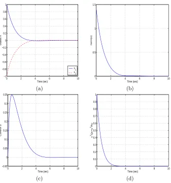
We first consider the system behavior when the initial condition is x0 = (1,−1)T. Figure 2(a)

depicts the state dynamics of the controlled system while Figure 2(b) is the norm of the state dynamics. Not only do the dynamics exhibit decay to zero, but the graph of the norm exhibits exponential decay. Figure 2(c) is the control and Figure 2(d) is the value of the cost functional integrand over time.

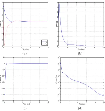
The second initial condition that we consider is x0 = (5,0)T. We find that, despite this initial

0 2 4 6 8 10 −1

−0.8 −0.6 −0.4 −0.2 0 0.2 0.4 0.6 0.8 1

States x

Time (sec)

x₁ x₂

0 2 4 6 8 10

0 0.5 1 1.5

norm(x)

Time (sec)

(a) (b)

0 2 4 6 8 10

−0.05 0 0.05 0.1 0.15 0.2 0.25 0.3 0.35

Control u

Time (sec)

0 2 4 6 8 10

0 0.1 0.2 0.3 0.4 0.5 0.6 0.7 0.8 0.9 1

x

TQx+u TRu

Time (sec)

(c) (d)

0 2 4 6 8 10 −8

−6 −4 −2 0 2 4 6

States x

Time (sec)

x₁ x₂

0 2 4 6 8 10

0 1 2 3 4 5 6 7 8 9

norm(x)

Time (sec)

(a) (b)

0 2 4 6 8 10

−300 −250 −200 −150 −100 −50 0 50

Control u

Time (sec) 0 2 4 6 8 10

10−8 10−6 10−4 10−2 100 102 104 106

x

TQx+u TRu

Time (sec)

(c) (d)

3

Numerical Methods for Solving SDRE

In Section 2.1, we presented an example for which the solution of the SDRE could be found analytically. In general one cannot find an exact solution analytically. Currently, one approach for solving the SDRE is via symbolic software packages such as Macsyma or Mathematica. However, once the dynamics of the system become complicated it is difficult to obtain a solution in this manner and it becomes necessary to approximate the solution. The method we describe in Section 3.1, referred to as the Taylor series method [7], works for systems with constant control coefficients (B

is not dependent on x). This uses the methodology of Taylor series approximations and is only effective locally. The interpolation method, presented in Section 3.2, can be used for more complex systems. This method involves varying the state over the domain of interest, solving for and storing the controlu(x), the SDRE solution Π(x), or the SDRE gainK(x) in a grid and interpolating over the stored solutions to approximate the control.

3.1 Taylor Series Method

The Taylor series method is used to synthesize controls for systems of the form

˙

x=A(x)x+Bu,

where the system has the same characteristics as (2) except thatB is constant. Since the control coefficients are constant, the SDRE has the form

Π(x)A(x) +AT(x)Π(x)₋Π(x)BR−1BTΠ(x) +Q= 0, (29)

whereQ andR are the matrices from the cost functional (1).

We rewrite the matrixA(x) as a sum of a constant matrix ˆAand a state-dependent incremental matrix ∆A(x), where we choose ˆA so that ( ˆA, B) is stabilizable. In order to form a series repre-sentation, the temporary variable ² (to be set to one upon completion of the series derivation) is introduced so that

A(x) = ˆA+²∆A(x).

We also represent the solution of the SDRE as the Taylor series

Π(x, ²) = Π(x)_|²=0+

∂Π(x)

∂²

¯ ¯ ¯ ¯

²=0

²+ ∂

2_Π(x)

∂²2

¯ ¯ ¯ ¯

²=0 ²2

2 +. . .

=

∞ X

n=0

²nLn(x),

where eachLn matrix is symmetric as a result of the symmetry of Π(x).

Substitution of these representations for A(x) and Π(x) into (29) yields

Ã_∞ X

n=0

²nLn(x) !

( ˆA+²∆A(x)) + ( ˆA+²∆A(x))T

Ã_∞ X

n=0

²nLn(x) !

− Ã_∞

X

n=0

²nLn(x) !

BR−1BT

à _∞ X

n=0

²nLn(x) !

Grouping like powers of ² and setting the coefficients to zero, we obtain an iterative method for finding the Ln matrices. This iteration scheme is

L0Aˆ+ ˆATL0−L0BR−1BTL0+Q = 0, (30)

L1( ˆA−BR−1BTL0) + ( ˆAT −BR−1BTL0)L1+L0∆A+ ∆AL0 = 0, (31)

Ln( ˆA−BR−1BTL0) + ( ˆAT −BTR−1BL0)Ln+Ln−1∆A +∆AT_L

n−1−Pn− 1

k=1LkBR−1BTLn−k

= 0. (32)

We note that equation (30) is the ARE corresponding to ( ˆA, B) while equations (31) and (32) are state-dependent Lyapunov equations. This algorithm converges locally to the solution of the SDRE under the assumptions that A(x) and B(x) are continuous [32]. This system of equations simplifies even further if ∆A(x) =g(x)∆AC, where ∆Ac is a constant matrix. By defining

Ln(x) = (g(x))n(Ln)C,

with (Ln)C a constant matrix, we obtain the simplified iterative scheme

L0Aˆ+ ˆATL0−L0BR−1BTL0+Q = 0,

(L1)C( ˆA−BR−1BTL0) + ( ˆAT −BR−1BTL0)(L1)C+L0∆AC + ∆ACL0 = 0,

(Ln)C( ˆA−BR−1BTL0) + ( ˆAT −BTR−1BL0)(Ln)C+ (Ln−1)C∆AC

+∆AT_C(Ln−1)C−Pkn=1−1(Lk)CBR−1BT(Ln−k)C

= 0.

Therefore, whenA(x) is of this type, we can approximate Π(x) using constant matrices calculated offline by solving one constant ARE and a series of constant Lyapunov equations. The subsequent control (an approximation of (14)) is given by

uN(x) =₋R−1BT

à _N X

n=0

((g(x))n(Ln)C) !

x,

whereN is the number of members of the series computed offline.

If solving the Lyapunov equations in real-time is not feasible and ∆A(x) does not take on the form described above, only L0 and L1 can be computed numerically offline (without the use of

symbolic solutions to the state-dependent Lyapunov equations). To achieve this, we rewrite

A(x) = ˆA+

m X

j=1

fj(x)(∆Aj)C,

where fj(x) are the distinct nonlinear terms of A(x) and (∆Aj)C are the corresponding constant

matrix coefficients. If we assumeL1 can be written as

L1=

m X

j=1

fj(x)(Lj1)C,

group thefj(x) terms together for each j, and set the coefficients to zero, we can approximate the

solution to the SDRE by solving

L0Aˆ+ ˆATL0−L0BR−1BTL0+Q= 0,

(Lj₁)C( ˆA−BR−1BTL0) + ( ˆAT −BR−1BTL0)(Lj1)C

+L0(∆AjC) + (∆A j

The corresponding approximate control (u1 _{denoting that we use one term, in addition to L}

0, of

the Taylor series) is given by

u1(x) =₋R−1BT



L₀+ m X

j=1

Lj₁fj(x) 

x.

3.2 Interpolation Method

The interpolation method, alluded to in [21], involves formulating the SDRE control (u(x)), SDRE solution (Π(x)), or even the SDRE gain matrix (K(x)) at a number of states in the domain of consideration and creating a grid to interpolate over as the states vary. We are able to construct an interpolation grid because the solutions to the SDRE continuously depend on the state. This technique is similar in spirit to gain scheduling and an optimal control two point boundary value problem described in [16]. We now proceed to develop the method mathematically.

3.2.1 Interpolate the Control

Let Ω0 denote the set from which the initial conditions are chosen. We assume that the state space,

Ω, is such that the state trajectory for any initial condition,x0 ∈Ω0, is contained entirely in Ω. If n is the dimension of the state, we create a finite mesh, D, that varies each xi, i= 1, . . . , n over

Ω. At each ˆx _∈D, solve and store the resulting control, uxˆ. Thus, we have effectively created an

interpolation grid that can be used to estimate the control for any point in Ω. In other words, the control can be approximated by

u(x) = interp_{uˆx}

where interp_{*_}represents any type of interpolation (1-d, 2-d, cubic, linear, etc.).

3.2.2 Interpolate over Π(x)

In SDC form, we find that the number of state variables on which A(x) andB(x) depend is often less than the dimension of the system. Let Ω0 and Ω be defined as above. Ifn is the dimension of

the state, we denote the r_≤nstates present inA(x) andB(x) as Ξ =_{xi1, ..., xir}. If we create a

mesh,D, that varies over eachxij ∈Ξ over the bounds imposed by Ω, solve and store the resulting

constant SDRE for each x_∈D, we have effectively created an interpolation grid for each element of Π(x). Thus, to estimate the solution to the SDRE for any point in Ω, we can interpolate over the elements of the grid. Thus, we can approximate the control with

u(x) =₋R−1BT(x)



 

interp_{π11(x)} . . . interp{π1n(x)}

..

. . .. ...

interp_{πn1(x)} . . . interp{πnn(x)} 

 x,

where interp_{*_} is defined as above. Since Π(x) is symmetric, we have interp_{πij} = interp{πji}

and the number ofr-degree interpolations is then n(n+ 1)/2.

Remark 3.1. We make the following comments regarding the interpolation method:

(ii) Interpolation over Π(x) is advantageous when the number of states, r, in Ξ is less than n. The degree of the interpolation is less for each element of Π(x) and the elements not present in Ξ do not have bounds invoked by the mesh.

(iii) Interpolation overu(x) is advantageous when the number of states,r, in Ξ is equal tonsince both meshes will impose bounds on all states and the interpolation is of the same complexity.

(iv) If nm _≤ n(n+ 1)/2, where m is the dimension of the control, then the interpo-lation method can be used with the gain matrix, K(x) to decrease the number of interpolations needed.

(iv) Not only can the interpolation method be used for nonconstant B(x), but it can also be used in more complex SDRE formulations that have nonconstant weighting matrices,Q(x) andR(x), in the cost functional.

3.3 Example 1 Revisited: Numerical Approximations

In Section 2.1 the exact solution to (26), (27) was used for the control of the system. We now use the numerical methods introduced in the previous section to approximate the solution to the SDRE, synthesize controls based on the approximations, and compare the results to the exact solution. To generate the Taylor series, we use the same representations as in Section 2 to split A(x) into a constant and state-dependent part. Therefore, we have

ˆ

A=

·

0 1 0 0

¸

, ∆A(x) =

·

0 0 1 0

¸

x2₁.

Since ∆A(x) =ACg(x), we can generate as many terms of the Taylor series offline as desired. For

the interpolation methods (bothu(x) and Π(x)), we create four grids INTu1, INTu2, INTPI1, and INTPI2 generated by two different meshes; one that uses a constant increment and another that focuses more attention (a finer mesh) closer to zero. Specifically, the first meshD1(corresponding to

INTu1 and INTPI1), is varied from [-5,5] in steps of 0.5 whereas the second mesh,D2(corresponding

to INTu2 and INTPI2), takes the values x _{∈ {−}5,₋3.5,₋2.5,2.5,3.5,5_{} ∪ {−}1 : 0.25 : 1_}, where

{a:b:c_} indicates incrementing fromato c in steps ofb. For interpolating the control, u(x), we vary bothx1 and x2 over the values in each mesh and for Π(x) we only varyx1 sincex2 does not

appear inA(x).

As mentioned in Section 3.1, there are limitations when using the Taylor series method for approximating the SDRE outside of a small interval about the origin. For instance, in [7], the approximate SDRE control fails for the system (26), (27) with initial conditions x0 = (2,0)T and x0 = (4,0)T. This occurs when five terms of the Taylor series method are used to approximate

Π(x). The instability can be examined more completely if we consider the maximum real part of the eigenvalues of the closed loop matrix A(x)₋BK(x) over an interval of x1. If the maximum

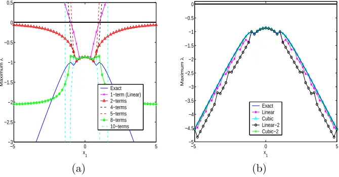
real part of these eigenvalues crosses the y-axis, the estimation for Π(x) is not only inaccurate but also causes the system to become unstable. Figure 4(a) depicts the maximum real part of the eigenvalues of A(x)₋BK(x) over x1 ∈ {−5 : 0.2 : 5} when Taylor series of different lengths

−5 0 5 −3

−2.5 −2 −1.5 −1 −0.5 0 0.5

x₁

Maximum

λ

Exact 1−term (Linear) 2−terms 4−terms 5−terms 8−terms 10−terms

−5 0 5

−5 −4.5 −4 −3.5 −3 −2.5 −2 −1.5 −1 −0.5 0

x₁

Maximum

λ

Exact Linear Cubic Linear−2 Cubic−2

(a) (b)

Figure 4: Maximum real part of the eigenvalues of the closed loop control matrix for (a) Taylor series method and (b) Π(x) interpolation grids INTPI1 and INTPI2.

not a surprise that there were difficulties using the control for the system with the initial condition (2,0)T _{and (4,0)}T_{. We see from this example that using more terms in the Taylor series will not}

necessarily result in more accuracy. For instance, we observe that the use of the 8-term expansion in control formulation results in a closed loop system that remains stable for the entire interval whereas the 10-term series results in an unstable closed loop system outside of a small region of the origin. For the sake of comparison, we provide the plot for the maximum real part of the eigenvalues of the closed loop control for the interpolation method (over Π(x)) in Figure 4(b). Here, the maximum real part of the eigenvalues is close to exact for both cubic and linear interpolation for the entire interval.

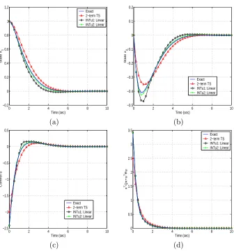
Next, to study the accuracy of all of the numerical approaches, we use the approximate feedback controls to stabilize the system from a number of initial conditions. Since the 2-term and 8-term Taylor series produce the only stable closed loop systems, we present the results for the controls generated with these two series. We use initial conditions close to the origin and relatively far from the origin, so as to compare the Taylor series method to the interpolation method in both situations. These initial conditions are (1,0)T _{and (3,3)}T_{, respectively.}

Table 3.3 lists the floating point operation count (FLOPS) needed at each time step to compute the control, the 2-norm of the difference between the numerical method and the exact solution, and the value of (26) for both initial conditions. Since INTu2 does not have a uniform mesh, it requires more FLOPS to use interpolation. As can be seen in the table, one 2-d cubic interpolation foru(x) is more costly than the three 1-d cubic interpolations for the Π(x) grid and the control formulated using the Π(x) grid is also the most accurate for both types of interpolation. Figures 5(a), 5(b), 5(c), and 5(d) represent the states x1 and x2, the control, and the cost functional integrand for

this example with the initial condition x0 = (1,0)T. The solutions presented graphically are the

Method FLOPS D1 C1 D2 C2

Exact 22 0.000 1.967 0.000 7.677_×102

2-term TS 34 2.933_×10−1 1.833 9.872 1.231_×103

8-term TS 100 1.105_×10−1 2.246 4.722 7.717_×1014

INTu1: Linear 39 2.466_×10−1 2.009 3.637_×10−1 7.688_×102 INTu1: Cubic 475 3.623_×10−2 _{1.964 2.492×10}−2 _7.676×102

INTPI1: Linear 69 9.062_×10−2 _{1.980 1.047×10}−1 _7.682×102

INTPI1: Cubic 162 5.334_×10−3 _{1.967 5.909×10}−3 _7.677×102

INTu2: Linear 121 6.564_×10−2 _{1.976 2.112 8.401×10}2

INTu2: Cubic 6935 1.556_×10−3 _{1.966 3.541×10}−2 _7.681×102

INTPI2: Linear 138 2.420_×10−2 1.970 7.587_×10−1 7.914_×102 INTPI2: Cubic 2280 1.011_×10−4 1.967 1.628_×10−2 7.683_×102

Table 1: Comparison of Numerical Methods, FLOPS - the floating point operations needed to compute the control for one time step, the 2-norm of the difference of the approximate state trajectory and the exact trajectory for (D1) x0 = (1,0)T and (D2) x0 = (3,3)T, and the value of

the cost functional integrand for (C1) x0= (1,0)T and (C2) x0= (3,3)T.

and subsequent dynamics are closer to those generated by the exact solution than those generated by the uniform grid (INTu1). The Taylor series approach also produces a control that is similar to the exact for this relatively local initial condition.

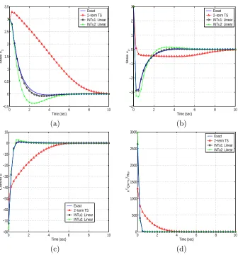
The second initial condition, (3,3)T _{is further from the origin. However, all of the methods}

produce stabilizing controls. Figures 6(a), 6(b), 6(c), and 6(d) represent the states x1 and x2, the

control, and the cost integrand for this initial condition. The Taylor series method depicted (as well as the 8-term, not depicted) produces an approximate feedback control that is far from accurate. The interpolation method produces relatively accurate controls without much computational effort.

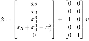
3.4 5D Example

To illustrate a case when interpolating over Π(x) or K(x) is more beneficial, we consider the following example from [31]. The system is

˙

x=



    

x2

x3

x3₄ x5+x34−x21

0



    

+



    

0 0 0 0 1 0 0 0 0 1



    

u. (33)

Associated with these dynamics, we choose the quadratic cost functional weighting matrices in (1) to beQ= 10I5×5 and R= 0.1I2×2.

Here, we use an obvious SDC parameterization

A(x) =



    

0 1 0 0 0

0 0 1 0 0

0 0 0 x2

4 0

−x1 0 0 x24 1

0 0 0 0 0



0 2 4 6 8 10 −0.2

0 0.2 0.4 0.6 0.8 1 1.2

Time (sec)

State x

1

Exact 2−term TS INTu1: Linear INTu2: Linear

0 2 4 6 8 10

−0.5 −0.4 −0.3 −0.2 −0.1 0 0.1 0.2

Time (sec)

State x

2

Exact 2−term TS INTu1: Linear INTu2: Linear

(a) (b)

0 2 4 6 8 10

−2.5 −2 −1.5 −1 −0.5 0 0.5

Time (sec)

Control u

Exact 2−term TS INTu1: Linear INTu2: Linear

0 2 4 6 8 10

0 0.5 1 1.5 2 2.5 3 3.5

Time (sec)

x

TQx+u TRu

Exact 2−term TS INTu1: Linear INTu2: Linear

(c) (d)

Figure 5: Comparison of Taylor series and interpolation methods for 2D example, closed loop state dynamics for (a)x1 and (b) x2, (c) control u, and (d) cost functional integrand over the time span

0 2 4 6 8 10 −0.5

0 0.5 1 1.5 2 2.5 3 3.5

Time (sec)

State x

1

Exact 2−term TS INTu1: Linear INTu2: Linear

0 2 4 6 8 10

−4 −3 −2 −1 0 1 2 3

Time (sec)

State x

2

Exact 2−term TS INTu1: Linear INTu2: Linear

(a) (b)

0 2 4 6 8 10

−80 −70 −60 −50 −40 −30 −20 −10 0 10

Time (sec)

Control u

Exact 2−term TS INTu1: Linear INTu2: Linear

0 2 4 6 8 10

0 500 1000 1500 2000 2500 3000

Time (sec)

x

TQx+u TRu

Exact 2−term TS INTu1: Linear INTu2: Linear

(c) (d)

Figure 6: Comparison of Taylor series and interpolation methods for 2D example, closed loop state dynamics for (a) x1 and (b) x2, (c) control u, and (d) cost functional integrand from 0 ≤t ≤10

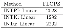
Method FLOPS INTPI: Linear 2028

INTK: Linear 1292

INTu: Linear 2202

Table 2: Comparison of interpolation methods for 5D example.

The firstn= 5 columns of the state-dependent controllability matrix are

M(x) =



    

0 0 0 0 1 0 0 1 0 0 1 0 0 0 0 0 0 0 1 0 0 1 0 0 0



    

which has rank n. There are only two states present in the A(x) matrix so that Ξ = _{x1, x4}.

Hence, when creating the Π(x) andK(x) grids (INTPI and INTK, respectively), we need only vary over those two particular states. Both of the grids use the mesh

D14={x1=−2 : 0.5 : 2} × {x4=−2 : 0.2 : 2}.

When creating the grid for interpolation over u, we must create a grid in five dimensions. This task is accomplished by crossing the D14 mesh with Dj = {xj = −2 : 1 : 2}, j = 2,3,5.

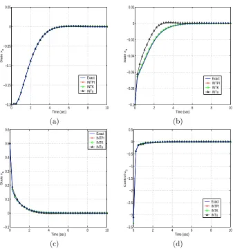
There-fore, the offline calculations take more time and computational effort to produce the grid. The control is formulated at each time step by either two 5D linear interpolations for u, ten 2D linear interpolations for K(x) or fifteen 2D linear interpolations for Π(x). Because of the complexity of 5D interpolations, interpolation over theugrid is not only less accurate but more computationally taxing. Figures 7(a)–(d) represent states x2, x4, x5, and control u2 respectively. The number of

FLOPS that it took to formulate the control at each time step for the different methods is given in Table 2. Here, interpolation over the gain matrix K(x) is clearly the most accurate and least computationally taxing. Note that in each of the following two examples the “exact” solution is obtained by solving the SDRE evaluated at the state (so that it is an ARE) at each time increment of the integration.

3.5 3D Example

The last example we present is referred to as the toy example [13]. We present this example because it exhibits complexities not yet encountered in the previous examples. First, it has nonconstant weighting matrices for the state. Specifically, we seek to minimize the cost functional

J(x0, u) =

Z ∞

0

xTQ(x)x+uTRu dt

where

Q(x) = 0.01





0 0 0

0 ex1 ₁

0 1 e−x1



,

with respect to the state dynamics

˙

x1 = f1(x)

˙

x2 = e−x1x3+e−x1/2u

˙

x3 = −ex1x2+ex1/2u

0 2 4 6 8 10 −0.2

−0.15 −0.1 −0.05 0 0.05

Time (sec)

State x

2

Exact INTPI INTK INTu

0 2 4 6 8 10

−0.1 −0.08 −0.06 −0.04 −0.02 0 0.02

Time (sec)

State x

4

Exact INTPI INTK INTu

(a) (b)

0 2 4 6 8 10

−0.1 0 0.1 0.2 0.3 0.4 0.5 0.6

Time (sec)

State x

5

Exact INTPI INTK INTu

0 2 4 6 8 10

−3.5 −3 −2.5 −2 −1.5 −1 −0.5 0 0.5

Time (sec)

Control u

2

Exact INTPI INTK INTu

(c) (d)

−0.0520 0 0.05 40

60 80 100 120 140 160

f_c

c1

−0.0520 0 0.05 40

60 80 100 120 140 160

f_c

c1

(a) (b)

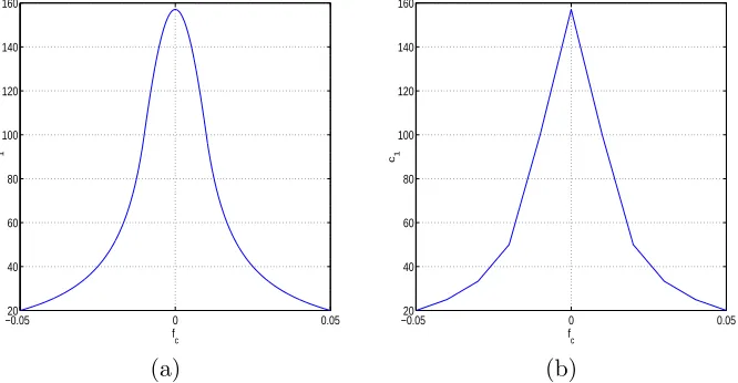
Figure 8: c1 withfc step size (a) 0.0001 and (b) 0.01.

where

f1(x) =χ[−3,3](x1)sgn(ex1x22−e−x1x23).

Second, since the dynamics are not continuous we must use an approximate continuous parameter-ization to formulate the SDRE control. As detailed in [13], thex1 dynamics used to formulate the

control are approximated and stabilized using

˙

x1≈satsin(fc)−x1,

where

satsin(θ) =

 



sin¡_πθ

2δ

¢

if _|θ_|< δ

1 if θ_≥δ

−1 if θ_{≤ −}δ ,

fc=ex1x22−e−x1x23,

and δ= 0.001. Then, defining

c1= satsin_fc(fc), c2 = e x₁

−1

x1 , and c3 =

e−x₁

−1

x1 ,

we can rewrite the dynamics used to formulate the control as

˙

x1 ≈ c1(c2x1+ 1)x22−c1(c3x1+ 1)x23−x1

˙

x2 = (c3x1+ 1)x3+e−x1/2u

˙

x3 = −(c2x1+ 1)x2+ex1/2

This introduces the last complexity that is of importance. The limits of c1, c2, and c3 as fc and

x1 go to zero exist (and are 2/(δπ), 1, and −1 respectively) and, hence, each are well behaved.

However, as we increase the increment of fc from 0.0001 to 0.01, it decreases the appearance of

continuity in c1 (see Figure 8). Therefore, the grid step size must be kept reasonably small to keep

Method FLOPS INTPI: Linear 1413

INTK: Linear 696

INTu: Linear 246

Table 3: Comparison of interpolation methods for 3D example.

order to integrate the system with the exact solution (the SDRE being solved at each time step) for some initial conditions.

By (4), we can parameterize these dynamics in many ways. In [13] (here we correct a mistake made therein), the terms with more than one multiple of the state are represented as

c1c2x1x22 = α1(c1c2x22)x1+ (1−α1)(c1c2x1x2)x2, c1c3x1x23 = α2(c1c3x23)x1+ (1−α2)(c1c3x1x3)x3,

c3x1x3 = α3(c3x1)x3+ (1−α3)(c3x3)x1,

c2x1x2 = α4(c2x2)x1+ (1−α4)(c2x1)x2.

(34)

We chooseα1=α2 = 0 andα3=α4 = 1 resulting in the parameterization

A(x) =





−1 c1c2x1x2+c1x2 −c1c3x1x3−c1x3

c3x3 0 1

−c2x2 −1 0





and

B(x) =





0

e−x1/2

ex1/2



.

The grids that we use result from varyingx1,x2 and x3 over the mesh D={−3.5 : 0.2 : 3.5}. As

depicted in Figure 9, interpolation over Π(x),K(x), andu(x) all stabilize the system. The FLOPS needed to compute the solution for each method are given in Table 3. Since u(x) only requires one interpolation, it is evident that interpolation over this grid is the most efficient method to approximate the control.

4

Nonlinear Estimation

We now extend the SDRE theory for state feedback to state estimation. This is of particular interest for nonlinear systems with state-dependent output coefficients. Specifically, for systems that can be put in the form

˙

x=f(x) =A(x)x, (35)

wherex_{∈ <}n _{and f(x) is nonlinear with output given by}

y =C(x)x, (36)

whereC(x) is a continuous m_×n matrix-valued function. From [14], we see that a system of the form

˙

xe=A(xe)xe+ Ψ(xe,(C(x)x−C(xe)xe)) (37)

0 5 10 15 20 −3.5

−3 −2.5 −2 −1.5 −1 −0.5 0

Time (sec)

State x

1

Exact INTPI INTK INTu

0 5 10 15 20

−0.2 −0.1 0 0.1 0.2 0.3 0.4 0.5 0.6

Time (sec)

State x

2

Exact INTPI INTK INTu

(a) (b)

0 5 10 15 20

−0.2 0 0.2 0.4 0.6 0.8 1 1.2

Time (sec)

State x

3

Exact INTPI INTK INTu

0 2 4 6 8 10

−3.5 −3 −2.5 −2 −1.5 −1 −0.5 0 0.5

Time (sec)

Control u

2

Exact INTPI INTK INTu

(c) (d)

Figure 9: Comparison of interpolation methods for 3D example, closed loop state dynamics for (a)

We can now formulate the proposed nonlinear estimator by mimicking the theory of estimators for linear systems. If the system were linear, it is well known that the optimal observer is given by

Ψ(z,(Cx₋Cz)) =L(Cx₋Cz),

whereL= ΓCT_V−1_{and Γ solves the ARE for the dual system. Likewise, under certain assumptions,}

we obtain a suboptimal observer for the nonlinear system by exploiting the dual system. Hence, to find the suboptimal observer, we consider the cost functional

J(ˆx,uˆ) = 1

2

Z ∞

0

ˆ

xTUxˆ+ ˆuTVu dt,ˆ (38)

with associated state dynamics given by

˙ˆ

x=AT(ˆx)ˆx+CT(ˆx)ˆu,

whereU _{∈ <}n×n is SPSD andV _{∈ <}m×m is SPD. Similar to the linear theory, we choose Ψ(xe,(C(x)x−C(xe)xe)) =L(xe)(C(x)x−C(xe)xe),

where

L(xe) = Γ(xe)CT(xe)V−1 (39)

and Γ(xe) solves the dual SDRE,

Γ(xe)AT(xe) +A(xe)Γ(xe)−Γ(xe)CT(xe)V−1C(xe)Γ(xe) +U = 0. (40)

The system with the proposed observer is given by

˙

x = A(x)x, (41)

˙

xe = A(xe)xe+L(xe)(y−C(xe)xe), (42)

y = C(x)x. (43)

(44)

It remains to be shown that the error for the system is asymptotically stable to zero. To develop the theory, we require the following remarks and observations:

Remark 4.1. The observer based SDRE has a solution at each x in the state domain, including

x= 0.

Define A0 =A(0) andC0 =C(0). Then, the solution at x= 0, Γ0, is the solution to the ARE

Γ0AT0 +A0Γ0−Γ0C0TV−1C0Γ0+U = 0. (45)

Therefore, each of the state-dependent matrices can be represented by the maps

A(x) =A0+ ∆A(x),

C(x) =C0+ ∆C(x),

and

It follows directly that

L(x) =L0+ ∆L(x),

where

L0 = Γ0C0TV−1 (46)

and

∆L(x) = (∆Γ(x)CT(x) + Γ0∆CT(x))V−1.

Here,L0 is the gain matrix that stabilizes (AT0, C0T). Consequently, A0−L0C0 has all eigenvalues

with negative real parts. Also, since ∆A(x), ∆C(x), and ∆Γ(x) are zero atx= 0 and continuous, they are small and bounded in a neighborhood of the origin. As a result, ∆L(0) = 0 and ∆L(x) is small in a neighborhood of the origin.

We are now able to prove the following theorem:

Theorem 4.1. Assume that f(x) and ∂f_∂x(x)

j (j = 1, . . . , n) are continuous in x for all kxk ≤ r,ˆ

ˆ

r > 0 and that x = 0 is a stable equilibrium point of (41). Additionally assume that f(x) and

y(x) can be put into SDC form such that f(x) =A(x)x and y(x) =C(x)x where (A(x), C(x)) is a detectable parameterization and A(x) and C(x) are locally Lipschitz for all x _∈Ω_{⊆ Br}(0), where

Ω is a nonempty neighborhood of the origin. Then the estimated state given by

˙

xe =A(xe)xe+L(xe)(C(x)x−C(xe)xe), (47)

(where L(x) is given by (39)) will converge locally asymptotically to the state.

Proof. Let r >0 be the largest radius such that _Br(0)_⊆Ω. As in the linear case, we consider the error between the actual state and the estimated state given by

e(t) =x(t)₋xe(t).

The error must satisfy the differential equation

˙

e(t) = ˙x(t)₋x˙e(t),

with the initial conditione0 =e(0) =x0−xe0, wherex0 =x(0) andxe0 =xe(0). Substituting the

state (35) and state estimator dynamics (47) into the error dynamics yields,

˙

e = A(x)x₋A(xe)xe−L(xe)(C(x)x−C(xe)xe)

= (A0−L0C0)e+ ∆A(x)x−∆A(xe)xe

−L(xe)(∆C(x)x−∆C(xe)xe)−∆L(xe)C0e.

We set

g(x, xe, e) = ∆A(x)x−∆A(xe)xe

−L(xe)(∆C(x)x−∆C(xe)xe) −∆L(xe)C0e.

(48)

By the hypotheses that A(x) is locally Lipschitz on Ω, there exists aκA>0 such that

kA(x)₋A(xe)k ≤κAkek.

This Lipschitz condition extends to ∆A(x) =A(x)₋A0 so that

This, in turn, implies that

k∆A(x)x₋∆A(xe)xek=k∆A(x)x−∆A(xe)x

+ ∆A(xe)x−∆A(xe)xek ≤(κ_Akx_k+_k∆A(xe)k)kek.

By the conditions placed on C(x) there exists a Lipschitz constant, κC, such that (upon the same

manipulation as above)

k∆C(x)x₋∆C(xe)xek ≤(κCkxk+k∆C(xe)k)kek.

For notational brevity, we set

h(x, xe) = (κAkxk+k∆A(xe)k+κCkxkkL(xe)k

+_k∆C(xe)kkL(xe)k+k∆L(xe)kkC0k)

and conclude that

kg(x, xe, e)k ≤h(x, xe)kek. (49)

By construction of the incremental matrices,

lim

x,xe→0

h(x, xe) = 0.

Due to the detectability condition at the origin and the use of SDRE (and due to construction, LQR) techniques to find the gain, L0, there existsβ >0 andG >0 such that

kexp(A0−L0C0)k ≤Gexp(−βt).

Then, given η _∈ (0, β/G) let ² _∈ (0, r) be such that h(z,zˆ) _≤ η for all z,zˆ _{∈ B²}(0) _⊆ Ω. The equilibrium x = 0 is stable implying that there exists a δ _∈(0, ²/2] such that _kx(t)_k < ²/2 for all time so long as _kx0k< δ. Letx0 and e0 be such x0 ∈ Bδ(0)⊆Ω ande0 ∈ Bˆ²(0), where ˆ²=²/(2 ˆG)

and ˆG= max_{G,1_}. Then the error dynamics have a local solution and are still contained in_Br(0), possibly on only a small interval [0,˜t), and so long as the solution exists it can be expressed by the variations of constants formula

e(t) = exp((A0−L0C0)t)e(0)

+

Z t

0

exp((A0−L0C0)(t−s))g(x(s), xe(s), e(s))ds.

(50)

By continuity there exists some finite time ˆt _∈ ¡

0,t˜¤

such that e(t) is in the ball _B²/2(0). Then,

upon taking the norm of both sides of (50), we find that for allt_∈[0,ˆt)

ke(t)_{k ≤}Gexp(₋βt)_ke(0)_k+Gη

Z t

0

exp(₋β(t₋s))_ke(s)_kds. (51)

We now multiply by exp(βt) and apply the Gronwall inequality so that, fort_∈[0,ˆt),

and it follows that

ke(t)_{k ≤}G_ke0kexp((Gη−β)t). (53)

By the choice we have made for e0 then

ke(t)_{k ≤} ²

2exp((Gη−β)t). (54)

But the boundη holds only as long asxe(t) remains inB²(0). However, because kxe(t)k − kx(t)k ≤ ke(t)_k,

kxe(t)k ≤

²

2+

²

2exp((Gη−β)t). (55)

Hence, byη < β/G, xe stays in B²(0) for all time and the state estimator converges exponentially

to the state.

4.1 State Estimator Example One

This example is a simple demonstration of the SDRE technique for state estimation. The system that we wish to observe (from [29]) is given by

˙

x1 = x2x21+x2,

˙

x2 = −x31−x1,

y = x1.

In SDC form, the above system can be rewritten as

˙

x =

·

0 1 +x2

1

−(1 +x2₁) 0

¸

x

y = £

1 0¤

x.

The state-dependent observability matrix is

O(x) =

·

1 0

0 1 +x2₁

¸

.

Since O(x) has full rank throughout _<2, the system is observable.

We set the weighting matrices in (38) to U = 10I and V = 0.01. We use the interpolation method to approximate Γ(x) where the estimator mesh is Mx = {−2 : 0.1 : 2}. We use an

initial condition of x0 = (1,1)T for the state and xe0 = (0.5,0.5)T for the estimated state. As a

comparison, we also display the state estimator found in [29] given by

˙

z1=−5z1+z2+ 5y+z1z22

˙

z2=−11z1−z13+ 10y

which we refer to as the Thau estimate (for this system). Figures 10(a) and (b) exhibit the fast convergence of each state estimate tox1 andx2. Figure 10(c) is a state-space representation of the

0 2 4 6 8 10 −1

−0.5 0 0.5 1 1.5

Time (sec)

State x

1

Actual State Thau Estimate SDRE Estimate

0 2 4 6 8 10

−1 −0.5 0 0.5 1

Time (sec)

State x

2

Actual State Thau Estimate SDRE Estimate

(a) (b)

−1 −0.5 0 0.5 1 1.5 −1

−0.5 0 0.5 1

State x₁

State x

2

Actual State Thau Estimate SDRE Estimate

0 2 4 6 8 10

0.1 0.2 0.3 0.4 0.5 0.6 0.7

Time (sec)

Error

Thau Error SDRE Error

(c) (d)

Figure 10: Plots for Example 4.1, (a) statex1 with the Thau and SDRE estimates of x1, (b) state x2 with the Thau and SDRE estimates of x2, (c) state-space representations x2 vs. x1 for actual

4.2 State Estimator Example Two: Unstable Zero Equilibrium

We now present an example that shows the effectiveness of the estimator synthesized through the use of SDRE techniques even when the hypotheses of the theorem are not satisfied. Consider the system

˙

x1=x2,

˙

x2=−x2|x2|, (56)

with measurement

y=x1.

Lyapunov stability theory states that if there exists a Lyapunov function, V, such that in every neighborhood of the origin V and ˙V have the same sign, then the origin is unstable. Using the Lyapunov function V(x) =_kx_k2₂ we see that

˙

V(x) =x1x˙1+x2x˙2

=x1x2−x22|x2|.

If we let ² _∈ (0,1) and consider the vector ˆx = (²/2, ²/2)T _{∈ B²(0). Then, V(ˆx) > 0 and since}

²2_≤²,

˙

V(ˆx) = ²

2

µ

²

2−

²2

4

¶

>0.

Therefore, zero is unstable for the given system and this violates the hypotheses of the theorem. However, numerically we shall show that the state estimator constructed with SDRE techniques works very well. As a comparison, we consider the following second order estimator from [29] (we will again refer to this as the Thau state estimator):

˙

z1 =−20z1+z2+ 10y,

˙

z2 =−100z1−z2|z2|+ 100y.

We can rewrite (56) in the SDC form f(x) =A(x)x where

A(x) =

·

0 1

0 _−|x2|

¸

.

Since

C=£

1 0¤

,

the state-dependent observability matrix isO(x) =I, so we have that this system is observable for allx. For the weighting matrices in (38), we useU = 50I andV = 0.1. To approximate the solution to the SDRE, we use the interpolation method for Π(x) and the mesh used is Mx ={−5 : 0.2 : 5}.

We set the initial condition of the state to x0 = (1,1)T and the initial condition of each state

estimator toxe0 = (0,0)T. Figure 11 depicts the behavior of the Thau and SDRE state estimators

over a five second time span. Figure 11(a) exhibits the fast convergence of each state estimator to

x1, where Figure 11(b) conveys that each state estimator takes more time to converge to x2. The

0 1 2 3 4 5 0

0.5 1 1.5 2 2.5 3

Time (sec)

State x

1

Actual State Thau Estimate SDRE Estimate

0 1 2 3 4 5

0 0.5 1 1.5 2 2.5 3 3.5

Time (sec)

State x

2

Actual State Thau Estimate SDRE Estimate

(a) (b)

0 0.5 1 1.5 2 2.5 3 0

0.5 1 1.5 2 2.5 3 3.5

State x₁

State x

2

Actual State Thau Estimate SDRE Estimate

0 1 2 3 4 5

0 0.5 1 1.5 2 2.5

Time (sec)

Error

Thau Error SDRE Error

(c) (d)

Figure 11: Plots for Example 4.2, (a) statex1with the Thau and SDRE estimates ofx1, (b) statex2

with the Thau and SDRE estimates ofx2, (c) state-space representations x2 vs. x1 for actual state

and state estimators, and (d) norm of the error, _ke(t)_k2, for the Thau and SDRE state estimators

over the time span 0 _≤ t_≤ 5 with state initial condition x0 = (1,1)T and state estimator initial

5

Compensation Using the SDRE State Estimator

In this section, we investigate the use of the SDRE state estimator in state feedback control laws to compensate given nonlinear systems. We consider systems that can be put in the SDC form

˙

x=A(x)x+B(x)u,

y=C(x)x,

where A(x) is a continuous n_×n matrix-valued function, B(x) is a continuous n_×m matrix-valued function and C(x) is a continuous p_×n matrix-valued function. We denote Π(x) as the solution to (12), where Q and R are the matrices from the cost functional (1) and Γ(x) as the solution to (40), where U and V are the matrices from the cost functional (38). If we again let

L(x) = Γ(x)CT(x)V−1 and K(x) =R−1BT(x)Π(x), the control using estimator compensation can be formulated as

˙

x = A(x)x₋B(x)K(xe)xe,

˙

xe = A(xe)xe−B(xe)K(xe)xe+L(xe)(y−C(xe)xe),

y = C(x)x.

(57)

To show that the compensated system converges asymptotically to zero in a neighborhood about the origin, we require the following remarks:

Remark 5.1. The block matrix

° ° ° ° · A B C D ¸° ° ° °≤ ° ° ° ° · A 0 0 0 ¸° ° ° ° + ° ° ° ° · 0 B 0 0 ¸° ° ° ° + ° ° ° ° · 0 0 C 0 ¸° ° ° ° + ° ° ° ° · 0 0 0 D ¸° ° ° °

=_kA_k+_kB_k+_kC_k+_kD_k

(58)

Remark 5.2. The matrix

H(x) =

·

A(x)₋B(x)K(x) 0

0 A(x)₋L(x)C(x)

¸

has all eigenvalues with negative real part for allx such that the state-dependent controllability and observability matrices have full rank. This follows directly from the eigenvalue separation property [1], since at each x, H(x) is a constant block diagonal matrix and the blocks each have eigenvalues with real part negative.

We are now able to prove the following theorem for the compensated system:

Theorem 5.1. Assume that the system

˙

x=f(x) +B(x)u

is such that f(x) and ∂f_∂x(x)

j (j = 1, . . . , n) are continuous in x for all kxk ≤ r,ˆ ˆr > 0, and that

f(x) can be written as f(x) = A(x)x (in SDC form). Assume further that A(x) and B(x) are continuous. If A(x), B(x), and C(x) are chosen such that the pair (A(x), C(x)) is detectable and

(A(x), B(x)) is stabilizable for all x _∈ Ω _{⊆ B}rˆ(0) (where Ω is a nonempty neighborhood of the

origin), then (ˆx,ˆe) = (0,0) for system (57) is locally asymptotically stable. Here, e=x₋xe is the

Proof. Letr >0 be the largest radius such that_Br(0)_⊆Ω. Using the mapping techniques described in the preceding proofs, one has

A(x) =A0+ ∆A(x),

B(x) =B0+ ∆B(x),

C(x) =C0+ ∆C(x),

K(x) =K0+ ∆K(x),

L(x) =L0+ ∆L(x),

with L0 = L(0) and ∆L(0) = 0 (etc.) for all of the matrices. The error between the actual state

and the estimated state satisfies the differential equation

˙

e(t) = ˙x(t)₋x˙e(t),

withe(0) =x(0)₋xe(0). We substitute the state and state estimator dynamics (57) for ˙x and ˙xe

yielding

˙

e = A(x)x₋A(xe)xe−(B(x)−B(xe))K(xe)xe

−L(xe)(C(x)x−C(xe)xe) (59)

As in the theory of linear systems, the dynamics of both e(t) andx(t) are of interest. Hence, the system to be considered is

˙

·

x(t)

e(t)

¸

,

with ˙x defined in (57) and ˙egiven by (59). In order to proceed, it is convenient to put the system into the form

˙

·

x(t)

e(t)

¸

=

·

H11 H12

H21 H22

¸ ·

x(t)

e(t)

¸

+

·

S11(x, xe) S12(x, xe)

S21(x, xe) S22(x, xe)

¸ ·

x(t)

e(t)

¸

. (60)

Rewriting the state dynamics with the given maps, we have that

˙

x= (A0−B0K0)x+ ∆A(x)x−B0∆K(xe)xe−∆B(x)K(xe)xe.

To put this in the proper form, we add and subtract the terms B0∆K(xe)x and ∆B(x)K(xe)x

resulting in

˙

x = (A0−B0K0)x+ ∆A(x)x−B0∆K(xe)x+B0∆K(xe)e

−∆B(x)K(xe)x+ ∆B(x)K(xe)e.

Thus,

H11 = A0−B0K0,

S11(x, xe) = ∆A(x)−B0∆K(xe)−∆B(x)K(xe),

H12 = 0,

S12(x, xe) = B0∆K(xe) + ∆B(x)K(xe).

Now we seek to formulate the error dynamics in a suitable manner. Rewriting the error dynamics with the given mappings yields

˙

e = (A0−L0C0)e+ ∆A(x)x−∆A(xe)xe

We eliminate all of terms withxe multiples by adding and subtracting terms (if the term consists

of a matrix timesxe we add and subtract that matrix timesx). This leaves us with

˙

e = (A0−L0C0)e+ ∆A(x)x+ ∆A(xe)e−∆A(xe)x

−(∆B(x)₋∆B(xe))K(xe)x+ (∆B(x)−∆B(xe))K(xe)e −∆L(xe)∆C(x)x+ ∆L(xe)∆C(xe)x−∆L(xe)∆C(xe)e −∆L(xe)C0e−L0∆C(x)x+L0∆C(xe)x−L0∆C(xe)e.

Thus, we have manipulated the error dynamics as desired and we have that

H21 = 0,

S21(x, xe) = ∆A(x)−∆A(xe)−∆B(x)K(xe) + ∆B(xe)K(xe) −∆L(xe)∆C(x) + ∆L(xe)∆C(xe)−L0∆C(x)

+L0∆C(xe),

H22 = A0−L0C0,

S22(x, xe) = ∆A(xe) + ∆B(x)K(xe)−∆B(xe)K(xe) −∆L(xe)∆C(xe)−∆L(xe)C0−L0∆C(xe).

Let

¯

H =

·

H11 H12

H21 H22

¸

and

¯

S(x, xe) =

·

S11(x, xe) S12(x, xe)

S21(x, xe) S22(x, xe)

¸

.

By Remark 5.1, we can bound the matrix norm by

kS¯(x, xe)k ≤ kS11(x, xe)k+kS12(x, xe)k+kS21(x, xe)k+kS22(x, xe)k.

Then, taking the norm of each of these matrices, we find

kS11(x, xe)k ≤ k∆A(x)k+kB0kk∆K(xe)k+k∆B(x)kkK(xe)k, kS21(x, xe)k ≤ k∆A(x)k+k∆A(xe)k+k∆B(x)kkK(xe)k

+_k∆B(xe)kkK(xe)k+k∆L(xe)kk∆C(x)k

+_k∆L(xe)kk∆C(xe)k+kL0kk∆C(x)k+kL0kk∆C(xe)k, kS12(x, xe)k ≤ kB0kk∆K(xe)k+k∆B(x)kkK(xe)k,

kS22(x, xe)k ≤ k∆A(xe)k+k∆B(x)kkK(xe)k+k∆B(xe)kkK(xe)k

+_k∆L(xe)kk∆C(xe)k+k∆L(xe)kkC0k

+_kL0kk∆C(xe)k.

Therefore,

kS¯(x, xe)k ≤ 2(k∆A(x)k+k∆A(xe)k) + 2kB0kk∆K(xe)k

+2_kK(xe)k(2k∆B(x)k+k∆B(xe)k) + 2k∆L(xe)kk∆C(xe)k

+_k∆L(xe)kk∆C(x)k+kL0k(2k∆C(xe)k+k∆C(x)k)

+_kC0kk∆L(xe)k

= g(x, xe).

By definition of the incremental matrices, as x, xe → 0, g(x, xe) → 0. Thus, for any η > 0 there

exists an α_∈(0, r) so that ifz,zˆ_{∈ B}α(0) then