DOI: 10.1534/genetics.106.067348
A Unified Model for Functional and Statistical Epistasis and Its
Application in Quantitative Trait Loci Analysis
Jose´ M. A
´ lvarez-Castro
1and O
¨ rjan Carlborg
Linnaeus Centre for Bioinformatics, Uppsala University, SE-75124 Uppsala, Sweden Manuscript received October 25, 2006
Accepted for publication March 20, 2007
ABSTRACT
Interaction between genes, or epistasis, is found to be common and it is a key concept for understanding adaptation and evolution of natural populations, response to selection in breeding programs, and deter-mination of complex disease. Currently, two independent classes of models are used to study epistasis. Statistical models focus on maintaining desired statistical properties for detection and estimation of genetic effects and for the decomposition of genetic variance using average effects of allele substitutions in popu-lations as parameters. Functional models focus on the evolutionary consequences of the attributes of the genotype–phenotype map using natural effects of allele substitutions as parameters. Here we provide a new, general and unified model framework: the natural and orthogonal interactions (NOIA) model. NOIA im-plements tools for transforming genetic effects measured in one population to the ones of other populations
(e.g., between two experimental designs for QTL) and parameters of statistical and functional epistasis into
each other (thus enabling us to obtain functional estimates of QTL), as demonstrated numerically. We develop graphical interpretations of functional and statistical models as regressions of the genotypic values on the gene content, which illustrates the difference between the models—the constraint on the slope of the functional regression—and when the models are equivalent. Furthermore, we use our theoretical foun-dations to conceptually clarify functional and statistical epistasis, discuss the advantages of NOIA over pre-vious theory, and stress the importance of linking functional and statistical models.
T
RADITIONALLY, most of the theory to study the evolution and genetic architecture of quantitative traits has been built on the assumption of additivity across the loci that contribute to the expression of a trait (Bu¨ rger2000). Interest in how interacting genes contribute to multifactorial trait expression is increas-ing in both quantitative and evolutionary genetics as it has been shown that gene effects commonly interact and that the effect of those interactions on the evo-lution and artificial selection of traits is far from neg-ligible (Carlborgand Haley2004; Hansen2006). We use the term epistasis to refer to nonadditivity in the contributions of several genes to a trait, meaning that the effects of the alleles of one gene depend on the ge-netic background (Phillips1998; Wagneret al.1998; Wadeet al.2001). This allows additive effects of genes (or allele substitutions) to evolve and the effect of partic-ular loci to range from being of crucial importance to completely vanishing changing backgrounds (Carlborg and Haley2004; Carlborget al.2006). Epistasis is there-fore critical in the understanding of the evolution of nat-ural populations, the response to selection in animal and plant breeding programs, and the genetic factorsunder-lying multifactorial disease (Templeton 2000; Moore and Williams2005). Thus, theoretical models of evolu-tion including epistasis may become more useful espe-cially in the light of the new molecular and statistical tools available for the study of allelic effects.
The term statistical epistasis refers to the use of sta-tistical tools to analyze gene interactions. Fisher(1918) provided the basis of the study of gene effects of a trait using parameters that represent the average effects of allele substitutions over the population and lead to a de-composition of the genetic variance. Cockerham(1954) and Kempthorne(1954) complemented this work with a subdivision of the epistatic variance into separate com-ponents. Fisher(1958) perceived epistasis as a nuisance effect whose evolutionary consequences would thus be equivalent to those of environmental variation. Albeit such an approach could be suitable to study phenotypic change in very large random-mating populations, it might not be reasonable otherwise. In fact, the theory of speciation by hybrid incompatibilities (Dobzhansky 1936; Muller 1942) and the shifting balance theory (Wright 1931, 1977) are two major theories that ex-emplify the crucial role of epistasis as a driving force in evolution. The evolutionary consequences of epistasis in the context of these theories, and in general in specia-tion and in adaptaspecia-tion in subdivided populaspecia-tions, have been studied by inspecting the components of the 1Corresponding author: Linnaeus Centre for Bioinformatics, Uppsala
University, Bio Medical Centre Box 598, SE-75124 Uppsala, Sweden. E-mail: [email protected]
genetic variance (Goodnight1988, 1995, 2000; Wade and Goodnight 1998; Barton and Turelli 2004; Turelliand Barton2006).
Cheverud and Routman (1995) and Cheverud (2000) analyze and discuss the efficiency of statistical epistasis for studying the evolution of complex traits. They underline the difference between genotypic and genetic values and suggest to study epistasis by focusing on genotypic values, as they represent natural effects of allele substitutions regardless of the allele frequencies in the population under study. Their view is in accor-dance with the first definition of the term epistasis by Bateson(1909), and they refer to this as physiological epistasis because the aim is to capture the interactions of the genes at the level of the organism rather than at a population level (see Phillips1998 for a comprehen-sive, historical dissection of this duality). Hansenand Wagner(2001b) further inspected the relationship be-tween physiological and statistical epistasis. They prefer to use the term functional epistasis—instead of physio-logical epistasis—as it reflects the functional properties of the gene interactions in determining the expression of a trait. Their multilinear model incorporates this in the form of a simplified genotype–phenotype map based on genetic values that capture the main role of gene interactions in evolution. The loss of generality of the multilinear model is rewarded by analytical tractability. A key concept in Hansenand Wagner’s (2001b) devel-opment is their change-of-reference tool, which allows the description of epistatic interactions as allele substi-tutions made on any reference genotype. In particular, this allows inspection of evolutionary properties of a pop-ulation by means of describing the (multilinear) epistasis parameters using the mean of the population as a re-ference point (Hansenand Wagner2001a; Hermisson et al. 2003; Carter et al. 2005; Hansen et al. 2006). Bartonand Turelli(2004) have developed a model to analyze the consequences of epistasis in the presence of genetic drift. Their theoretical framework comple-ments that of Hansenand Wagner(2001b) and imple-ments a new notation with the purpose of providing more transparent results than the previous approaches. Functional—or physiological—epistasis has also been referred to as biological epistasis, and has even been split into genetical epistasis and biological epistasis, when discussing how to integrate systems biology and quantitative trait loci (QTL) analysis (Moore 2005; Mooreand Williams2005).
In the context of QTL analysis, Yang(2004) and Zeng and collaborators (Kao and Zeng 2002; Zeng et al. 2005) have reviewed and analyzed several statistical mod-els used for obtaining estimates of epistasis. For two ma-jor reasons, they stress the use of orthogonal–statistical models. First, the measurement of genetic effects of re-duced models is consistent in orthogonal models. This enables a straightforward comparison of nested models for performing model selection. Second, each genetic
effect in an orthogonal model can be independently estimated and plays a role in the computation of its com-ponent of variance alone. Zeng et al. (2005) have de-veloped the G2A model, a multilocus two-allele model that is orthogonal in populations under strict Hardy– Weinberg and linkage equilibrium, regardless of the fre-quencies of the alleles at each locus. Wangand Zeng (2006) have extended this model to a multiallele frame-work with linkage disequilibrium, particularly focusing on the decomposition of the genetic variance. Yang (2004) has built an explicit two-locus two-allele model that is generally orthogonal regarding the frequencies of the genotypes in the populations and has imple-mented it with a tool for measuring the bias in the esti-mates of genetic effects caused by linkage disequilibrium. Here we establish a formal link between the models of statistical and functional epistasis through a unified, formal framework—the natural and orthogonal inter-actions (NOIA) model. We provide a mathematical de-scription of genetic systems that leads to a conceptual interpretation of the relationship between statistical and functional epistasis and a set of explicit expressions to translate between statistical and functional estimates and between genetic effects in different populations. The resulting model incorporates general statistical and functional formulations of genotypic values on genetic effects that improve both the existing statistical and the functional models of gene interactions. We also provide a graphical interpretation of the functional formulation of NOIA, similar to that of the statistical models—as lin-ear weighted regressions of the genotypic values on the gene content (Fisher1918). The slope of the functional regression is constrained to the one of an unweighted regression, which provides a characterization of when the functional and the statistical formulations are equivalent.
THE NOIA MODEL
Modeling genetic effects as allele substitutions on one specific genotype:Consider a trait controlled by a number of diallelic loci,n. We begin by using a partic-ular genotype as a reference point to build a genotype– phenotype map for this trait. First we focus in one locus, locusA. Zenget al.(2005) discuss several maps for one locus and two alleles, and we basically follow their no-tation and nomenclature here,G¼SE, whereGis the vector of genotypic values (G11,G12,G22, the phenotypes
of the three genotypes for allelesA1andA2).Sis called
descriptions of the genetic system with different refer-ence points when describing the genotypic values of the individuals in terms of the genetic effects.
We begin by using a single genotype, sayG11, as a
re-ference point from which to measure the genetic effects, resulting in the following formulation of the model,G¼ SG11E:
G11
G12
G22 0 @
1 A¼
1 0 0
1 1 1
1 2 0
0 @
1 A
R a d 0 @
1
A: ð1Þ
The first column ofSG11illustrates that the phenotypes are measured as deviations from the reference point, hereR ¼G11. The second column illustrates that one
additive effect is added toRfor eachA2allele and the
third column that the dominance effect is added to the heterozygote. The genetic effects are thus effects of allelic substitutions on the reference genotype A1A1.
The extension of this NOIA functional formulation to several loci is obtained as the Kronecker product of the Smatrices of the single loci (appendix a). For two loci,A and B, with genetic-effect design matrices SA and SB, respectively, this reads
GAB ¼ ðSB5SAÞ EAB; ð2Þ
whereEABis the two-locus vector of genetic effects. Let us call SAB ¼SB5SA. By using the properties of the
Kronecker product we getS1
AB ¼ ðS
1
B 5SA1Þand, hence,
the genetic effects can be obtained by solving the system
EAB ¼ ðSB15SA1Þ GAB: ð3Þ
If SA¼SB ¼SG11, the formulations (2) and (3) de-scribe the effects of allelic substitutions on the reference genotypeA1A1B1B1(or simply ‘‘1111’’), as both loci have
G11as their respective reference points. This is
conve-nient for constructing the model, but insufficient for a functional genotype–phenotype map, which should be able to describe the genetic effects as effects of sub-stitutions from any reference point. Therefore, we im-plement the model with a change-of-reference tool.
Modeling genetic effects as allele substitutions on any genotype:Here we provide a simple way to compute the genetic-effect design matrix for using any individual of the population as a reference point of the genetic system. This enables us to describe all genotypic values in the genetic system as sets of allele substitutions on any particular (ref-erence) individual in the population and also to use the mean of the population under study as the reference point. The general expression for the one-locus functional genetic-effect design matrix,SF, is
SF¼
1 p122p22 p12
1 1p122p22 1p12
1 2p122p22 p12 0
B @
1 C
A; ð4Þ
where p11,p12, and p22are the genotypic frequencies.
This expression is derived in appendix b and its
(generally fictitious) reference point is R ¼ p11G11 1
p12G121p22G22. Expression (4) makes complete sense
whenRis the phenotype of any single genotype,e.g.,G11
by setting p11¼1,p12¼0,p22¼0. The extension to
the general multilocus case is obtained by using the Kronecker product of the genetic-effect matrices of the single loci, as in (2).
The inverse of matrix (4) is
SF1¼
p11 p12 p22
1
2 0 12
1
2 1
1 2 0
B @
1 C
A: ð5Þ
This expression is very useful to inspect some particular-ities of the one-locus and multilocus NOIA functional formulations. By equatingE in (1), the general expres-sion of the genetic effects of the one-locus system is E¼S1
F G. From this expression and (5) it becomes
clear that the reference point is in factR¼p11G111p12G12
1p22G22, and that the genetic effects are always defined
in the same way, regardless of the reference point used, asa¼1
2(G22G11),d ¼G12 1
2(G111G22). This is the
same definition of genetic effects as in, for instance, Cockerham’s F2model (Zenget al.2005). The general two-locus functional formulation of the NOIA model can be obtained by inserting two single-locus genetic-effect design matrices (4) in expression (2). In this expression (not shown), the frequencies at each locus affect the single-locus effects at the other locus. This is in accor-dance with the definition of epistasis—the effects of the allele substitutions at one gene depend on the genetic background. The (pairwise) epistatic effects in the two-locus case, on the other hand, are independent of the frequencies. This logic, only the highest-order effects being independent of the frequencies, extends to higher-order terms of epistasis when more loci are involved.
Translating genetic effects from one to another reference genotype:Expressions (4) and (5) enable us to change the reference point from which to describe the genetic effects. Given a description of the genetic system from reference pointR1,G¼SR1ER1, and a de-scription of the same genetic system from a different re-ference pointR2,G¼SR2ER2, it is straightforward to get to the expression
ER2¼ S
1
R2 SR1ER1 ð6Þ
by just inserting Gfrom the first description into the second one and equatingER2. This expression is useful to change the reference of the genetic effects, i.e., to translate the genetic effects associated with a reference point to the genetic effects associated with a different reference point.
ðp11¼p22Þ or ðp12¼0Þ: ð7Þ
This expression is derived inappendix cand its graph-ical interpretation is in the next section. For the populations fulfilling (7), the NOIA functional formu-lation is an orthogonal statistical formuformu-lation that can therefore be used to properly estimate genetic effects in QTL studies as justified by Yang(2004) and Zeng and collaborators (Kaoand Zeng2002; Zenget al.2005).
A general orthogonal–statistical model: The explicit and general orthogonal [regardless of whether or not condition (7) holds] expression of the statistical one-locus genetic-effect design matrix,SS, is
SS¼
1 p122p22
2p12p22
p111p22 ðp11p22Þ2
1 1p122p22
4p11p22
p111p22 ðp11p22Þ2
1 2p122p22
2p11p12
p111p22 ðp11p22Þ2 0
B B B B B B B @
1 C C C C C C C A :
ð8Þ
The scalars of theSSmatrix fulfill the conditions to be
orthogonal scalessensuCockerham(1954) (appendix c). The first two columns of the functional (4) and
sta-tistical (8) genetic-effect design matrices are the scalars of the reference point and the scales related to additive effects and are identical in the two formulations. The differences between the two one-locus formulations are in the third column, the scales for dominance. The ex-pressions for these dominance orthogonal scales can be obtained by computing the values of the dominance deviations in the graphical interpretation (appendix c). In the same way as in the functional formulation, the gen-eral one-locus statistical formulation of the NOIA model (8) can be easily extended to a general multilocus case by taking the Kronecker product of single-locus genetic-effect design matrices (2). This resembles the way it has been done for particular cases of statistical formulations (Zeng et al. 2005). The statistical formulation (8) re-duces to the functional one (4) whenever the conditions for orthogonality of the functional formulation (7) hold. The only exception is when the frequency of one of the genotypes is one, where the denominators in the third column of the statistical genetic-effect design matrix (8) are zero. This intuitively makes sense as no meaningful statistical formulation can be expected in a population in which only one genotype is present.
The inverse of matrix (8) is
S1 S ¼
p11 p12 p22
p11ðp1212p22Þ p111p22 ðp11p22Þ2
p12ðp11p22Þ p111p22 ðp11p22Þ2
p22ðp1212p11Þ p111p22 ðp11p22Þ2
1
2 1 12
0 B B B B B @
1 C C C C C A
:
ð9Þ
Unlike in the general functional formulation (5), the additive effects, reflected in the second row of this
in-verse matrix, change depending on the allele frequen-cies in the population. This is a consequence of the parameters of the model no longer being natural effects of allele substitutions, but instead average effects of allele substitutions over the population. To clarify the difference between the meaning of the parameters in the statistical and the functional model formulations, we useES¼(m,a,d)Tfor the genetic effects vector in the
one-locus statistical formulation instead ofEF¼(R,a,d)T
that was used in the functional formulation (1). InESwe
usem for denoting the mean of the population as in other statistical epistasis models (e.g., Zenget al.2005). However, we prefer to denote the statistical genetic effects as Greek letters for making a clear distinction between statistical and functional genetic effects. The vectorEF
follows the notation of the unweighted regression model by Cheverud and Routman (1995) regarding the functional genetic effects, although we prefer to useR instead ofCfor the reference point (Cheverud2000).
Taking into account this notation of the vectors of genetic effects, and interpreting the genetic-effect de-sign matrices as statistical matrices instead of functional matrices, expression (6) holds for the statistical formu-lation, and therefore it enables us to translate statistical genetic effects of one population into how they would look in a different population. The statistical formula-tion of the NOIA model (8) can be used for estimating multilocus genetic effects in the exact same way as pre-vious models (appendix c).
Obtaining functional estimates of genetic effects from statistical estimates:Let us denote bySFandEFthe
genetic-effect design matrix and the vector of genetic effects in the functional formulation and bySSandES
the corresponding ones in the statistical formulation. In the one-locus case, the vectors of genetic effects are EF¼(R,a,d)TandES¼(m,a,d)T. By implementing this
notation in (1) we have G¼SF EFandG¼SS ES.
Hence, the expressions for the transformations of ge-netic effects between the two formulations of the NOIA model are
EF¼SF1SSES; ES¼SS1SFEF: ð10Þ
These expressions resemble the translations of genetic effects between different reference points (6), but they have a different meaning. In fact, the transformations in (10) do not change the reference point of the system at all. Expressions for simultaneous translations of genetic effects, regarding both the reference point and the model formulation, can be easily obtained by combin-ing expressions (6) and (10).
PREVIOUS MODELS AS PARTICULAR CASES OF NOIA
The F2 and the F‘ models: One of the most
population, ideally with genotype frequenciesp11¼14,
p12¼12,p22¼14. The genetic-effects design matrix of the
F2 model can be obtained by inserting the genotype
frequencies of an ideal F2 population in the NOIA
statistical formulation (8), and its reference pointmis, thus, the mean of an F2population. For the multilocus
case, the description of the system is obtained by first computing the correct genetic-effect design matrices for the individual loci and then computing the Kronecker product of the single-locus genetic-effect design matri-ces, as shown in (2). The F‘model, which is orthogonal for—and thus adapts to the mean of—a population with frequenciesp11¼12,p12¼0,p22¼12, is also a particular
case of the general NOIA statistical formulation that can be explicitly obtained in the same way as explained for the F2model above. One unsurprising remark about the
F‘ population is that it fails in offering estimates of dominance effects, due to the absence of heterozygotes. The G2A model: Zeng et al. (2005) provided the genetic-effect design matrix of the G2A model for the one-locus case as
SG2A¼
1 2ð1pÞ 2ð1pÞ2
1 12p 2pð1pÞ
1 2p 2p2
0 B @
1 C
A; ð11Þ
wherepis the gene frequency of allele ‘‘1.’’ This model is a statistical formulation of genetic effects that is orthog-onal for populations under Hardy–Weinberg propor-tions. From (8), we can obtain a genetic-effect design matrix for a population under Hardy–Weinberg as a particular case of the NOIA statistical formulation. This reads
SHW¼
1 2ð1pÞ 2ð1pÞ2
1 112p 2pð1pÞ
1 2p 2p2
0 B @
1 C
A: ð12Þ
Matrices (11) and (12) differ only in the sign of the values of their second columns. This sign difference occurs because Zenget al. (2005) assume in all their models—following the notation by Falconer and MacKay(1996)—that allele ‘‘2’’ always leads to a lower genotypic value than allele 1. Therefore their estimates reflect the absolute value of the additive effects, by reporting the positive decrement of the genotypic value of an allele 1 to allele 2 substitution. In principle, this fits to the context of a QTL mapping experiment, in which allele 1 comes from the high line and allele 2 comes from the low line. It is, however, not a generally con-sistent formulation. Transgressive alleles are known to exist (Tanksley1993) and in an extension of the model to several loci with epistasis, the effect of the alleles could switch signs at two different genetic backgrounds—a phenomenon known as sign epistasis (Weinreichet al. 2005). In such situations, the estimates of genetic effects from the G2A model (Equation 11) remain positive when the allele substitutions decrease the genotypic
value, and they become negative when they increase it. On the contrary, the Hardy–Weinberg statistical formu-lation we obtain as a particular case of NOIA (Equation 12) is consistent with the direction of the allele sub-stitution, as NOIA always leads to adding values that are positive when they increase the genotypic values from allele 1 and negative when they decrease them.
The unweighted regression model: Cheverud and Routman’s (1995) unweighted regression model (see also Cheverud2000; Zeng et al.2005) is a particular case of NOIA in which p11¼p12¼p22¼13 for each locus.
Since—as well as for the F2and the F‘ models—these frequencies fulfill criterion (7), the unweighted regres-sion model can be considered as a particular case of both the functional (Equation 4) and the statistical (Equa-tion 8) formula(Equa-tions of NOIA. The reference point of this model is the unweighted mean of the genotypic val-ues of all genotypes,R¼(1/3)G111(1/3)G121(1/3)G22
and the definition of genetic effects is the same as in the F2model, as explained in relation to expression (5).
GRAPHICAL INTERPRETATION OF NOIA
Ideograph representing one-locus functional and statistical formulations: The main foundations of the NOIA model are presented in the ideograph in Figure 1. The functional (Equation 4) and the statistical (Equa-tion 8) formula(Equa-tions of genetic systems are represented by solid and shaded lines, respectively. The arrows point-ing to the right or up represent the way in which the model is developed in the previous section of this arti-cle. Starting from a single genotype,G11, as a reference
point, the model can be extended to a general func-tional formulation (solid line). Whenever criterion (7) holds—to the left of the vertical dashed line—the func-tional formulation is also an orthogonal–statistical for-mulation (shaded line). The F2model is one example of
such a model. An orthogonal–statistical formulation exists also when criterion (7) does not hold—to the right of the dashed line. The HW3 population (see
below) is an example of this other case. The genetic ef-fects can be easily translated between models by using the change-of-reference and transformation tools (6) and (10). The arrows pointing down or to the left represent how we translate genetic effects in a numerical example below.
substitutions—are the vertical distances from the re-gression line to the real values (Figures 2 and 3A). To-gether with the graphical interpretation of the average effects and the dominance deviations (aianddij, which are directly related to the decomposition of the genetic variance), we provide the expressions that give those values as functions of the parameters of the NOIA functional formulation—Greek letters. The additive variance is the variance of the average effects,ai, and the dominance variance is the variance of the domi-nance deviations,dij(Cockerham1954; Falconerand MacKay1996; Lynchand Walsh1998). The extension of this to several loci is straightforward. The additive-by-additive variance, for instance, is the variance of the additive-by-additive average effects,aaij, and these would be obtained in a multilocus genetic system as the pro-ducts of the additive-by-additive genetic effects and the corresponding orthogonal scales in the multilocus genetic-effect design matrix.
The criterion for overlapping functional and statis-tical formulations:The slope of the regression in Figure 2 equals the slope of the line defined by the genotypic values ofG11andG22. This is a result of the regression
being made on an ideal F2 population, where both
homozygotes have the same weight in the regression,p11
¼ p22 (¼ 14), thus making criterion (7) hold.
Conse-quently, the regression is parallel to the line throughG11
andG22 only when the functional formulation of the
NOIA model is orthogonal. In Figure 3A, the regression is made on what we label as an HW3 population, in
whichp1 ¼0.3 and the Hardy–Weinberg proportions
hold, thus leading top11¼0.09,p12¼0.42,p22¼0.49. In
this case criterion (7) does not hold, and the slope of the regression differs from the line defined byG11andG22,
leading to a change in the additive values. In this par-ticular case they even change signs.
A graphical interpretation of the functional formu-lation: The NOIA functional formulation can also be interpreted as a regression on the gene content, albeit this is not a typical linear regression anymore. Here, the slope of the regression remains constant regardless of the allele frequencies. In particular, it always remains at the same value as in the cases in which it is orthogonal—i.e., the slope of the line defined by G11 and G22 (Figures 2
and 3B). This is actually the same slope as for an unweighted regression on the gene content. This constraint of the functional regression becomes appar-ent when comparing Figure 3A with 3B. Figure 3A represents the statistical formulation, showing a normal least-squares linear regression in an HW3population, as
defined above, which is not parallel to the line through G11 and G22. Figure 3B represents the functional
re-gression (for the same population) that fits the data under the constraint of retaining the same slope as the regression in Figure 2,i.e., by being parallel to the line defined byG11 andG22. This constraint enables us to
perform the regression in populations in which one only genotype is present; i.e., it allows us to use one single genotype as a reference point of the functional formu-lation. This is not possible for the statistical formulation, as already commented above in relation to expression (8). The equivalent parameters toaianddijare, in the functional formulation, the additive effects of natural allele substitutions in individuals,ai, and the deviations from those,dij.
NUMERICAL EXAMPLE
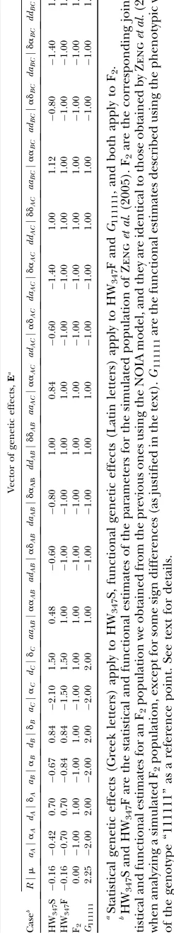
Here we apply the NOIA model to estimates from a QTL analysis on simulated data by Zenget al.(2005). The data consist of a single trait controlled by three bialle-lic loci with defined underlying additive and dominance effects and pairwise gene interactions. Two populations are simulated: an F2 population and a population
(HW347or H as in subscripts) where the three loci
fol-low Hardy–Weinberg proportions, with the frequencies of the 2 alleles being 0.3, 0.4, and 0.7 (see Tables 3 and 5 in Zenget al.2005). Zenget al.(2005) report different estimates of genetic effects for the same trait in the F2
and HW347simulated populations, explained by the fact
that they report statistical estimates representing the average effects of allele substitutions in the two pop-ulations. Those estimates are indeed properties of the populations as well as of the underlying genetic system. The statistical formulation of NOIA in QTL analysis: The statistical formulation of NOIA can be used in QTL analysis in the same way as other statistical models of Figure1.—Ideograph showing the main
founda-tions of the NOIA model for the one-locus case. The starting point is a description of the genetic effects as
allele substitutions on the reference genotypeG11
(solid circle). This description is extended to a gen-eral functional formulation (thick solid line) by means of the change-of-reference tool represented by the horizontal and the nearly horizontal arrows. The reference points for which criterion (7) holds are represented to the left of the vertical dashed line. For populations with those ref-erence points as mean phenotype, the functional formulation is orthogonal, and it coincides with the statistical formulation (thick shaded line). Other reference points may be represented to the right of the vertical dashed line. For populations with those reference points as mean phenotype, the two formulations do not coincide, and the transformation tool, represented by the vertical arrow, can be used to
transform the functional formulation into the statistical formulation and vice versa. The F2and the HW3populations, represented as
epistasis (appendix c). Here we show how to use NOIA to translate statistical estimates, as they come from the analysis of experimental data, into what would come from other experimental designs and into estimates of functional epistasis. Let us first consider the estimates of genetic effects Zenget al.(2005) obtained for a HW347 simulated population using the G2A model as a starting point. Following the logic of expressions (6) and (10), fromG¼SG2A EG2AandG¼SHW EHW, we obtain
EHW¼SHW1 SG2AEG2A to translate the G2A estimates
into what they would have been if the statistical formu-lation of NOIA had been used instead. The simulated populations in Zenget al.(2005) consisted of 100,000 individuals, meaning that the random departures from
the Hardy–Weinberg proportions are certainly negligi-ble and the G2A model is, thus, virtually orthogonal in the population under study. The only differences be-tween the G2A estimates and the NOIA estimates are, therefore, the signs of the additive effects (as illustrated when obtaining the G2A model as a particular case of NOIA). This can be seen in the first row of Table 1—the genetic effects obtained from Zenget al.(2005) are all positive.
Transformation from statistical into functional esti-mates:In the NOIA model, the statistical genetic effects of HW347 can be transformed into functional genetic
effects (‘‘HW347F,’’ second row in Table 1), as depicted
in the ideograph by the arrow labeled ‘‘transformation’’ Figure3.—Graphical interpretation of the parameters of
the NOIA model for an HW3 population, with frequencies
p11 ¼ 0.09, p12 ¼ 0.42, p22 ¼ 0.49, in the one-locus case.
(A) Statistical formulation. All the symbols have the same meaning as in Figure 2. The regression on the gene content (thick shaded line) does not have the same slope as the
(dashed) line through G11 and G22, and therefore it does
not coincide with the functional regression of the same pop-ulation (shown below). This happens when the frequencies of the population do not fulfill condition (7), as shown in the
ideograph (above). The reference point, R¼ 1.33, occurs
at gene content 1.4. (B) Functional formulation. All the sym-bols have the same meaning as in Figures 2 and 3A. The re-gression on the gene content (thick solid line) is forced to be
parallel to the (dashed) line throughG11andG22and would
have a different slope otherwise (see statistical regression of the same population above). However, the reference point is the same as in the statistical regression.
Figure2.—Graphical interpretation of the parameters of
the NOIA model for an F2population in the one-locus case.
The values of the parameters come from a regression of the
genotypic values (G11,G12,G22) on the gene content. These
genotypic values are represented as solid circles, and their size is determined by their frequency in the population. We show a case of strong overdominance because it allows us to better visualize the parameters of interest. The functional regression (thick solid line) is constrained to have the same slope as the
(dashed) line throughG11andG22. The statistical regression
(thick shaded line) is a weighted linear regression on the gene content, and under condition (7) it has the same slope
as the line throughG11andG22. In this case, therefore, the
functional and statistical regressions coincide. The elements
of theS ¼ (sij) matrix are the natural and the orthogonal
scales, in the functional and the statistical model formula-tions, respectively. Latin letters are the functional genetic ef-fects, and Greek letters are the statistical genetic effects. The
reference point,R¼1.25, is represented by a triangle. It is the
intercept of the regressions and it occurs at the average gene content, which in this case is one. It is the starting point from
which to measure the additive effects (aI¼ai). The deviations
of the regression, the dominance deviations (dij¼dij) would
in Figure 1. This is done using (10), which for this particular case becomesEHF¼SHF1SHSEHS, where H
represents HW347, F represents functional, and S
re-presents statistical in the subscripts. The genetic-effect design matrices needed for the operation are the Kronecker products of the matrices for the individual loci as in (2) and as in (B10) inappendix b.A,B, andC are the three biallelic loci affecting the trait and the frequencies of theA2,B2, andC2alleles areqA¼0.3,qB¼
0.4, andqC ¼0.7. Thus, we haveS1 HF ¼S
1 HFC5S
1 HFB5
SHF1A (utilizing that the Kronecker product is inter-changeable with the inverse operation) and SHS¼
SHSC5SHSB5SHSA, where the matrices for the
individ-ual loci are derived using expressions (4) and (5) for the functional formulation and (8) and (9) for the statistical formulation. The functional genetic effects in the re-sulting vectorEHFare the effects of allele substitutions
performed on a fictitious genotype whose genotypic value would be the mean of the HW347 population.
Thus, the reference point of the functional description has not changed after the transformation from the statistical description. We change the reference to the genotypic value of a real individual below in this section. Translating genetic effects into an ideal F2population:
In the HW347population, we do not consider the
func-tional genetic effects as being meaningfulper se. Here we use them as an intermediate step to compute—as de-picted in one of the change-of-reference arrows in the ideograph (Figure 1)—the genetic effects as they would appear in an ideal F2population (third row in Table 1).
These calculations are done using (6), here taking the formEF2 ¼S
1
F2 SHFEHF. The genetic-effect design ma-trices are computed as in (2) and (3), or more explicitly as in (B3) inappendix b, byS1
F2 ¼5
3
i¼1ðS
1
F jq¼0:5Þand
SHF¼SHFC5SHFB5SHFA, where the matrices of the
individual loci are again computed from (4) and (5). The vectorEF2 (third row in Table 1) gives the average effects of substitutions in an F2population. These are,
therefore, the values that would be obtained in a QTL experiment by means of the F2model in an ideal F2
population. And, in fact, these values are the same values Zenget al.(2005) estimate from an F2simulated population, built on the same genetic system (except for the sign differences in the genetic effects involving one additive effect, as explained above).
Genetic effects as allele substitutions on a particular genotype:Here we use the NOIA model to obtain esti-mates at the reference point of the phenotypic value of a real genotype, G111111. In this way, the functional
pa-rameters get a direct genetic interpretation as natural effects of allele substitutions made on one particular individual. We shorten G111111 to read R1 in the
sub-scripts, and hence expression (6) takes the formER1¼ S1
R1 SF2EF2, where S
1
R1 ¼5
3
i¼1ðS
1
F jp11¼1Þ and SF2¼
53i¼1ðSFjq¼0:5Þ. The functional estimates of genetic
effects as the natural effects of allele substitutions on the reference genotype G111111 (i.e., the resulting
ER1 vector) are shown in the last row of Table 1. These can of course be easily transformed into natural ef-fects of allele substitutions from any other reference genotype by means of another change of reference operation.
General remarks: All cases in Table 1, except form HW347S in the first row, are either purely functional or
both functional and statistical descriptions of a genetic system in which the highest level of epistasis present is pairwise epistasis. This is why, as pointed out above in relation to expression (5), all the genetic effects of the interactions remain constant throughout these cases. The additive and dominance effects, on the other hand, do not necessarily remain constant between cases in Table 1. The values of the genetic effects of a functional and a statistical description of the same population are different because of the different meaning of the parameters in the functional and the statistical formu-lations of the NOIA model. The values of the genetic effects of (functional or statistical) descriptions of the system from different reference points are different because the single-locus genetic effects depend on the genetic background—i.e., because of epistasis.
DISCUSSION
Conceptualizing and unifying functional and statis-tical epistasis:In our opinion, the use of the concepts of statistical epistasis and functional epistasis has some-times been misleading. Models of statistical epistasis were developed for performing orthogonal decompositions of variance in populations and for QTL detection and estimation. On the other hand, models of functional epistasis—also called physiological epistasis, biological epistasis, and genetical epistasis—were proposed to bet-ter analyze the role of gene inbet-teractions in evolution and to understand the genetic architecture underlying mul-tifactorial disease, but its relationship to statistical epis-tasis has not been entirely explored. The NOIA model provides the necessary theory to unite these concepts and allows us to gain new insights into how epistasis should be modeled and inspected. In the light of the two formulations of our model, the terms functional epis-tasis and statistical episepis-tasis can be viewed as two shadows cast from one object. We have characterized the situa-tions under which these two shadows completely coin-cide and developed tools to transform them into each other when they do not. Statistical formulations of ge-netic systems are built on orthogonal parameters that represent average effects of allele substitutions over pop-ulations, whereas functional formulations of genetic sys-tems are genotype–phenotype maps built on parameters that represent natural effects of allele substitutions on real or fictitious genotypes. Both of them are core mod-els of genetic effects (gene effects and gene interactions) that describe the genetic architecture underlying a trait
in two different ways and that are, therefore, suitable for different purposes.
Since NOIA overcomes the duality of functional and statistical models of epistasis, it enables us to obtain es-timates of both functional and statistical genetic effects from data. The NOIA statistical formulation achieves orthogonality regardless of the genotype frequencies in the population and is therefore convenient for QTL detection and estimation and for an orthogonal decom-position of the genetic variance. The NOIA model is implemented with a tool to transform those orthogonal estimates into functional estimates. When expressed from the mean of the population under study, these func-tional estimates represent effects of allele substitutions performed on a fictitious genotype. Using the change-of-reference tool of the NOIA model, the reference point of the functional formulation can be changed to any real genotype, and therefore the NOIA model handles natural effects of allele substitutions on those genotypes, which is the genuine point of functional models. All these possibilities are represented in Table 1 as the result of a numerical example that illustrates the practical use of the theory provided within this article. The transformations in Table 1 can be explained using the classical concepts of cell means and factor effects (Searle 1971; Coffman et al. 2005). Indeed, expres-sions (6) and (10) are based on the fact that the genetic values (cell means) remain constant and they can therefore be used for linking and translating between genetic (factor) effects that entail different interpreta-tions (statistical, functional, and both from different reference points).
The NOIA statistical formulation: The statistical formulation of the NOIA model is an explicit, orthog-onal description of multilocus two-allele models. Pre-vious statistical epistasis models can thus be obtained as particular cases of NOIA. Orthogonality is a key prop-erty for statistical epistasis models to be appropriate for QTL analysis methods based on model selection. The F‘ model, for instance, lacks this property in commonly used experimental populations (Kao and Zeng 2002; Yang2004; Zenget al.2005). The classical F2model, on the other hand, is orthogonal in ideal F2populations
in which the frequencies are p11¼14, p12¼12, p22¼14.
thus avoiding the bias caused by sampling errors and segregation distortion. Furthermore, by changing the reference of the orthogonal–statistical estimates to a common reference point in NOIA, it is possible to com-pare the estimates of genetic effects coming from dif-ferent QTL experiments affected by specific sampling errors or carried out using different experimental de-signs. This is an original feature of NOIA and we have proved its validity and accuracy by successfully trans-forming genetic effects between two simulated popula-tions with different genotype frequencies but the same underlying genetics (Table 1).
Yang’s (2004) genetic effects model can, like NOIA, deal with departures from the Hardy–Weinberg propor-tions, but his model is explicitly developed only for the two-locus case, whereas NOIA is not constrained regard-ing the number of loci. The epistasis model of Wang and Zeng(2006) is particularly focused on the decom-position of the genetic variance. Their model is more general than the current NOIA statistical formulation regarding the number of alleles and the computation of genetic covariances due to linkage disequilibrium. How-ever, this model is valid only for populations under strict Hardy–Weinberg proportions and not developed using the convenient algebraic notation that simplifies the computation of the model for the particular population under study. This notation (together with the generality regarding genotype frequencies) allows us, in particu-lar, to implement in NOIA a tool to translate, and there-fore to compare, statistical estimates of genetic effects, as explained above. Finally, Wangand Zeng’s (2006) model, the F2model, and the G2A model do not provide
a link between statistical epistasis and functional epista-sis, which is the main motivation for the NOIA model.
The NOIA functional formulation: The algebraic structure of the NOIA functional formulation resembles the statistical formulation but instead of being based on average effects of allele substitutions in populations, it uses natural (nonaverage) effects of allele substitutions as parameters. The graphical interpretation of these pa-rameters is also akin to the classical linear regression of the genotypic values on the gene content that defines the average effects (see Figures 2 and 3B). The connec-tion we provide between the funcconnec-tional and the statis-tical formulations enables us to feed the first one with estimates of genetic effects obtained by means of QTL mapping studies on biallelic systems, as explained in the text and illustrated by means of the numerical example. Several studies have analyzed general key properties of gene interactions using functional epistasis models. Hansen and collaborators, for instance, have found di-rectionality of gene interactions to determine the way in which short- and long-term genetic architecture evolves in the face of selection (Carter et al. 2005; Hansen 2006; Hansenet al.2006). The NOIA model enables us now to study directionality in particular traits of partic-ular populations, by using just data on orthogonal gene
interactions from QTL studies and transforming them into functional estimates in which directionality can be inspected.
Cheverud and Routman (1995; Cheverud 2000) made a challenging attempt in the direction of linking statistical and functional (physiological) epistasis. Their unweighted regression model can be understood as a simultaneously functional and statistical description of genetic effects for a specific reference point and can be obtained as a particular case of NOIA. However, their model is not implemented with a change-of-reference tool, which causes two major practical problems. First, as a statistical model of epistasis, it is only orthogonal (and therefore appropriate for QTL detection and estima-tion) in populations in which every single genotype is present in the same quantity. Second, as a functional model, it cannot deal with natural effects of allele sub-stitutions in real genotypes. In addition, several errors in the use and interpretation of the unweighted regres-sion model have been pointed out (Zenget al.2005). Hansen and Wagner’s (2001b) and Barton and Turelli’s (2004) functional epistasis models do incor-porate change-of-reference tools. The first one is for-mulated for multiple alleles and for constrained gene effects and interactions and the second one, like the current NOIA formulation, is a general formulation for two alleles. We find the algebraic notation of the NOIA functional formulation to be an advantage over these functional epistasis models. It is in fact by means of a parallel notation in the functional and the statistical formulations of the NOIA model that we developed both a graphical interpretation of functional epistasis and a transformation tool that enables us to feed the NOIA formulation with estimates of genetic effects from real data.
Future extensions of NOIA:As discussed above, the theoretical framework of the NOIA model presents considerable advantages over the previous formulations of epistasis, in particular in analysis of real QTL experi-ments. Consequently, we are in the process of imple-menting NOIA in the context of QTL interval mapping with Haley–Knott regressions (Haleyand Knott1992). We also aim to extend NOIA to multiple alleles and link-age disequilibrium, this last implementation motivated by the fact that even for unlinked loci, there is non-random association of alleles due to sampling in the experimental populations used in QTL mapping, re-sulting in biased estimates.
role of epistasis in evolution, the response to selection in animal and plant breeding programs, and the analysis of multifactorial disease. Marker-assisted selection is a promising strategy for improving selection response for traits that are difficult to measure in individuals used for breeding or that manifest themselves late in life. The efficiency of marker-assisted selection relies on the pre-cision with which estimates of genetic effects of indi-vidual or combinations of loci obtained in one genetic background can predict their effect in another. The generality of the NOIA model as well as its transforma-tion and change-of-reference tools can allow the breed-ers to estimate the genetic effects in one experimental design and use these estimates to predict the effect of the same locus or loci in a particular genotype of a breeding individual or an average effect in any breeding population. This cannot be done with the currently avail-able models. Another example where the NOIA model will fundamentally change the way science could pro-ceed is in the mapping of loci underlying multifactorial disease. For example, we are on the verge of performing massive association studies on a grand scale. In these studies, deviations from ideal population conditions in-clude sampling errors, segregation distortion, linkage disequilibrium, and (when the association studies are based on haplotypes) multiple alleles. The aim of these studies is to statistically detect loci affecting disease, but to functionally predict the effects of allele substitutions on an individual genotype basis to be able to suggest appropriate treatments or develop treatment regimes. The currently available models are far from suitable for this purpose, whereas the NOIA model is designed to do just this.
The authors thank Lars Ro¨nnega˚rd and Thomas Hansen for fruitful discussion. O¨ rjan Carlborg acknowledges funding from the Knut and Alice Wallenberg Foundation.
LITERATURE CITED
Barton, N. H., and M. Turelli, 2004 Effects of genetic drift on
var-iance components under a general model of epistasis. Evolution
58:2111–2132.
Bateson, W., 1909 Mendel’s Principles of Heredity.Cambridge
Univer-sity Press, Cambridge.
Bu¨ rger, R., 2000 The Mathematical Theory of Selection, Recombination
and Mutation.Wiley, Chichester, UK.
Carlborg, O., and C. S. Haley, 2004 Epistasis: Too often neglected
in complex trait studies? Nat. Rev. Genet.5:618–625.
Carlborg, O., L. Jacobsson, P. Ahgren, P. Siegeland L. Andersson,
2006 Epistasis and the release of genetic variation during long-term selection. Nat. Genet.38:418–420.
Carter, A. J., J. Hermissonand T. F. Hansen, 2005 The role of
ep-istatic gene interactions in the response to selection and the evo-lution of evolvability. Theor. Popul. Biol.68:179–196.
Cheverud, J. M., 2000 Detecting epistasis among quantitative trait
loci, pp. 58–81 inEpistasis and the Evolutionary Process, edited by J. B. Wolf, E. D. Brodieand M. J. Wade. Oxford University Press,
Oxford.
Cheverud, J. M., and E. J. Routman, 1995 Epistasis and its
con-tribution to genetic variance components. Genetics139:1455– 1461.
Cockerham, C. C., 1954 An extension of the concept of
partition-ing hereditary variance for analysis of covariances among rela-tives when epistasis is present. Genetics39:859–882.
Coffman, C. J., R. W. Doerge, K. L. Simonsen, K. M. Nichols, C. K.
Duarteet al., 2005 Model selection in binary trait locus
map-ping. Genetics170:1281–1297.
Dobzhansky, T., 1936 Studies on hybrid sterility. II. Localization of
sterility factors in Drosophila pseudoobscura hybrids. Genetics
21:113–135.
Falconer, D. S., and T. F. C. MacKay, 1996 Quantitative Genetics.
Prentice-Hall, Harlow, UK.
Fisher, R. A., 1918 The correlation between relatives on the
supposi-tion of Mendelian inheritance. Trans. R. Soc. Edinb.52:339–433.
Fisher, R. A., 1958 The Genetical Theory of Natural Selection.Dover,
New York.
Goodnight, C. J., 1988 Epistasis and the effect of founder events on
the additive genetic variance. Evolution42:441–454.
Goodnight, C. J., 1995 Epistasis and the increase in additive genetic
variance: implications for phase 1 of Wright’s shifting-balance theory. Evolution49:502–511.
Goodnight, C. J., 2000 Modeling gene interaction in structured
populations, pp. 129–145 inEpistasis and the Evolutionary Process, edited by J. B. Wolf, E. D. Brodieand M. J. Wade. Oxford
Uni-versity Press, Oxford.
Haley, C. S., and S. A. Knott, 1992 A simple regression method for
mapping quantitative trait loci in line crosses using flanking markers. Heredity69:315–324.
Hansen, T. F., 2006 The evolution of genetic architecture. Annu.
Rev. Ecol. Evol. Syst.37:123–157.
Hansen, T. F., and G. P. Wagner, 2001a Epistasis and the mutation
load: a measurement-theoretical approach. Genetics158:477–485.
Hansen, T. F., and G. P. Wagner, 2001b Modeling genetic
architec-ture: a multilinear theory of gene interaction. Theor. Popul. Biol.
59:61–86.
Hansen, T. F., J. M. A´lvarez-Castro, A. J. Carter, J. Hermissonand
G. P. Wagner, 2006 Evolution of genetic architecture under
directional selection. Evolution60:1523–1536.
Hermisson, J., T. F. Hansenand G. P. Wagner, 2003 Epistasis in
polygenic traits and the evolution of genetic architecture under stabilizing selection. Am. Nat.161:708–734.
Kao, C. H., and Z-B. Zeng, 2002 Modeling epistasis of quantitative
trait loci using Cockerham’s model. Genetics160:1243–1261.
Kempthorne, O., 1954 The correlation between relatives in a random
mating population. Proc. R. Soc. Lond. B Biol. Sci.143:102–113. Lynch, M., and B. Walsh, 1998 Genetics and Analysis of Quantitative
Traits.Sinauer, Sunderland, MA.
Moore, J. H., 2005 A global view of epistasis. Nat. Genet.37:13–14.
Moore, J. H., and S. M. Williams, 2005 Traversing the conceptual
divide between biological and statistical epistasis: systems biology and a more modern synthesis. BioEssays27:637–646.
Muller, H. J., 1942 Isolating mechanisms, evolution, and
tempera-ture. Biol. Symp.6:71–125.
Phillips, P. C., 1998 The language of gene interaction. Genetics
149:1167–1171.
Searle, S. R., 1971 Linear Models.Wiley, New York.
Tanksley, S. D., 1993 Mapping polygenes. Annu. Rev. Genet.27:
205–233.
Templeton, A. R., 2000 Epistasis and complex traits, pp. 41–57 in
Epistasis and the Evolutionary Process, edited by J. B. Wolf, E. D.
Brodieand M. J. Wade. Oxford University Press, Oxford.
Turelli, M., and N. H. Barton, 2006 Will population bottlenecks
and multilocus epistasis increase additive genetic variance? Evo-lution60:1763–1776.
Wade, M. J., and C. J. Goodnight, 1998 Genetics and adaptation in
metapopulations: when nature does many small experiments. Evolution52:1537–1553.
Wade, M. J., R. G. Winther, A. F. Agrawaland C. J. Goodnight,
2001 Alternative definitions of epistasis: dependence and inter-action. Trends Ecol. Evol.16:498–504.
Wagner, G. P., M. D. Laubichler and H. Bagheri-Chaichian,
1998 Genetic measurement of theory of epistatic effects. Ge-netica102–103:569–580.
Wang, T., and Z-B. Zeng, 2006 Models and partition of variance for
Weinreich, D. M., R. A. Watsonand L. Chao, 2005 Perspective:
sign epistasis and genetic constraint on evolutionary trajectories. Evolution59:1165–1174.
Wright,S.,1931 EvolutioninMendelianpopulations.Genetics16:93–159.
Wright, S., 1977 Experimental Results and Evolutionary Deductions
(Evolution and Genetics of Populations, Vol. III). University of Chicago Press, Chicago.
Yang, R.-C., 2004 Epistasis of quantitative trait loci under different
gene action models. Genetics167:1493–1505.
Zeng, Z-B., T. Wang and W. Zou, 2005 Modeling quantitative
trait loci and interpretation of models. Genetics 169: 1711– 1725.
Communicating editor: J. B. Walsh
APPENDIX A: THE NOIA MODEL FOR THE GENERAL MULTILOCUS CASE
To clarify the details of the general multilocus case, we first deal separately with the different components of the model, theGandEvectors and theSmatrix, and then combine them using an example. Although we use a functional formulation in the example, the guidelines for constructingG,E, andSare valid for both the functional and the statistical formulations.
The vector of genotypic values, G:The way in which the scalars of the vectorGare sorted can be obtained by means of the Kronecker product of the vectors of the single-locus genotypic vectors, in which we then substitute the products of single-locus genotypic values by the correspondent multilocus genotypic values, for instance,GB12(GA11byGA11B12, or simplyG1112). It is worth stressing that the Kronecker product of subsequent loci added to the genetic system must be
computed to the left of the previous ones, as shown in the example below, which makes the vector expand downward as new loci are considered.
The vector of genetic effects, E:This is obtained in a similar way as theGvector, by the Kronecker product of single-locus genetic effects vectors. In this case, we first replace the reference point by a one in the single-single-locus vectors and next compute the Kronecker product of the subsequent loci to the left of the previous ones. Then, to obtainEfrom the resulting vector, we just replace the products of the genetic effects by the corresponding interactions, for instance,dB (aAbyadABor by justadin the two-locus case), and the first scalar of the vector, which shall be one, by the reference pointR. Greek letters are used instead of the Latin letters in the statistical formulation. As was the case forG, to add new loci makes the vectorEexpand downward.
The genetic-effect design matrix, S: Once the single-locus genetic-effects design matrices are expressed at the desired single-locus reference point, the multilocusS matrix for the complete system can be obtained as the Kronecker product (for subsequent loci, to the left of the previous ones) of the single loci, as already explained in the text using expressions (2) and (3) and also inappendix busing (B3). We could also describe the system by multiplying theSmatrices of subsequent loci to the right of the previous ones. In this case the vectors of genotypic values and genetic effects would need to be sorted in a different way, in which the new scalars that appear due to considering new loci would have to be inserted before the previous ones, instead of afterward.
Example:Here we develop an example of a functional formulation using a real genotype as a reference point. Let us consider the simplest multilocus case, consisting of two loci,AandB, as in expression (2). This example deals with a very similar case to this expression,GAB¼ ðSB5SAÞ EAB, the only difference being that there we assumed that both genetic-effect design matrices came from expression (1), hence leading to GA11B11 or simply G1111, as reference, whereas in this example we use as a reference the phenotypic valueG1112instead. We follow the same order as above,
and therefore we begin by building the vector of genotypic values:
GB11
GB12
GB22
0 @
1 A5
GA11
GA12
GA22
0 @
1 A¼
GB11GA11
GB11GA12
GB11GA22
GB12GA11
GB12GA12
GB12GA22
GB22GA11
GB22GA12
GB22GA22
0 B B B B B B B B B B B B @
1 C C C C C C C C C C C C A
/GAB ¼
G1111
G1211
G2211
G1112
G1212
G2212
G1122
G1222
G2222 0 B B B B B B B B B B B B @
1 C C C C C C C C C C C C A
: ðA1Þ
1 aB
dB
0 @
1 A5
1 aA
dA
0 @
1 A¼
1 aA
dA
ab
aBaA
aBdA
dB
dBaA
dBdA
0 B B B B B B B B B B B B @
1 C C C C C C C C C C C C A
/EAB ¼
R aA
dA
aB
aa da dB
ad dd 0 B B B B B B B B B B B B @
1 C C C C C C C C C C C C A
: ðA2Þ
Here we use Latin letters, as in the functional formulation, but it works exactly the same for the statistical formulation, in which Greek letters are used instead. (A1) and (A2) are not the common ways in which the genotypic values and the genetic effects are sorted (see Table 1), but we find it convenient to use this configuration in our model for two main reasons. First, this way the vectors just extend downward whenever new loci are added to the genetic system. Second, it allows for a straightforward computation of the genetic-effect design matrix of the system, in which no rearrangement of its rows or columns is needed after computing the Kronecker product, as shown below. The single-locus genetic-effect design matrices for lociAandBareSA¼SG11andSB¼SG12 and are given in (1) and in (B7) inappendix b, respectively. Therefore, the two-locus genetic-effect design matrix is, by computing just the Kronecker product of these two matrices,
SAB ¼SB5SA¼
1 1 1
1 0 0
1 1 1
0 @
1 A5
1 0 0
1 1 1
1 2 0
0 @
1 A¼
1 0 0 1 0 0 1 0 0
1 1 1 1 1 1 1 1 1
1 2 0 1 2 0 1 2 0
1 0 0 0 0 0 0 0 0
1 1 1 0 0 0 0 0 0
1 2 0 0 0 0 0 0 0
1 0 0 1 0 0 1 0 0
1 1 1 1 1 1 1 1 1
1 2 0 1 2 0 1 2 0
0 B B B B B B B B B B B B @
1 C C C C C C C C C C C C A
: ðA3Þ
Here we can observe how the Kronecker product defines the natural scales of the gene interactions in a logical and structured manner. The scalars in boldface type in theSABmatrix come from multiplying the scalar in boldface type in theSBmatrix—at the column of the reference point,R—times theSAmatrix. The columns of the resulting submatrix have the same meaning as in theSAmatrix: they are coefficients ofR,aA, anddAfor the homozygotes for the 1 allele at locusB. The scalars in italics in theSABmatrix come from multiplying the scalar in italics in theSBmatrix—at the column of the additive effect,aB—times theSA matrix. The first column of the resulting submatrix has the same meaning as the scalar in italics in theSBmatrix: it is the additive effectaB. The other two columns are the scalars (the natural scales) of the interactions ofaBwith the genetic effects in the second and third columns of theSAmatrix: they are coefficients ofaaanddafor the same genotypes mentioned above. The interaction effect exists in an individual whenever the two interacting effects have nonzero natural scales in the one-locus matrices. This same logic applies to the other seven submatrices of dimension three in matrixSAB. The places in which the natural scales appear in theSAB matrix determine the way in which we sort the scalars of theGandEvectors.
From (A1), (A2), and (A3) we haveGAB¼SABEAB, which describes every genotypic value in a two-locus two-alleles genetic system as the result of a set of allele substitutions from the reference genotypeG1112.
APPENDIX B: THE CHANGE-OF-REFERENCE OPERATION
The functional change-of-reference operation: Recall that we have described a one-locus biallelic genetic system usingG11as a reference (Equation 1). Now, the genetic-effect design matrix that leads to a reference pointR2¼p11G111
p12G121p22G22,SR2, can be obtained from the genetic-effect design matrix for any other reference pointR1,SR1, as
SR2¼SR1PR2SR1I*; ðB1Þ
where the asterisk means that the first scalar of the identity matrix has been replaced by a zero, andPR2is the change-of-reference matrix for the reference point R2, a square matrix in which each column is filled with one of the
coefficients of the linear combination of genotypes that equals the new reference:
PR2¼
p11 p12 p22
p11 p12 p22
p11 p12 p22 0
@
1
A: ðB2Þ
It is worth pointing out that we consider only the cases in whichp111p121p22¼1, so that the scalars of the matrix can
be interpreted as frequencies of the genotypes in a population. We show below in thisappendixthat the change-of-reference operation (B1) consistently leads to the sameSR2matrix, independently of the starting reference pointR1 and, immediately afterward, we use an example to illustrate the logic that led us to this operation.
We obtained expression (4) by performing a change-of-reference operation as shown in (B1), withSR1¼SG11as in (1) and without specifying the values of the frequencies in the change-of-reference matrixPR2(B2). An extension to the general multilocus change-of-reference operation is straightforward. First the change of reference is performed separately for each locus, and then theSmatrix of the complete system is obtained from taking the Kronecker product of the new single-locus reference matrices, in reverse order. Fornloci this reads
SR12...Rn2 ¼5
1
i¼nSRi2; ðB3Þ
whereRi2is the reference points of locusi, andSRi2,i¼1,. . .,ncan be obtained as in (B1).
The transitive property: For the change-of-reference operation to be consistent, the resulting matrix of the particular reference point must remain the same, independently of the starting point from which it is computed. To show this we now prove the transitive property for the operation in Equation B1.
LetR1,R2, andR3be three reference points, and letPR2andPR3be the change-of-reference matrices ofR2andR3. We shall prove that changing the reference fromR1toR2, and afterward toR3, is the same as changing directly fromR1
toR3; that is, given
SR2¼SR1PR2SR1I* ðB4Þ
and
SR3¼SR2PR3SR2I*; ðB5Þ
we want to prove that
SR3¼SR1PR3SR1I*: ðB6Þ
By inserting (B4) into (B5), we get
SR3¼SR1PR2SR1I*PR3SR1I*1PR3PR2SR1I*I*:
Given thatI*I*¼I*,
SR3 ¼SR1PR3SR1I*1ðPR3IÞ PR2SR1I*:
Since the scalars in each row inPR3sum to one, then the scalars in each row in (PR3I) sum to zero. Since all the scalars inPR2are equal inside columns (say,liat columni), all the scalars in columniof the matrix (PR3I)PR2are 0(li). Hence, the matrix (PR3I)PR2is the zero matrix, and therefore (B6) is proved.
SG12 ¼SG11PG12SG11I*¼
1 0 0
1 1 1
1 2 0
0 B @
1 C
A
0 1 0
0 1 0
0 1 0
0 B @
1 C A
1 0 0
1 1 1
1 2 0
0 B @
1 C A
0 0 0
0 1 0
0 0 1
0 B @
1 C A
¼
1 0 0
1 1 1
1 2 0
0 B @
1 C
A
0 1 1
0 1 1
0 1 1
0 B @
1 C A¼
1 1 1
1 0 0
1 1 1
0 B @
1 C
A: ðB7Þ
The new matrix,SG12, is the result of subtracting toSG11, a matrix in which scalars are equal inside columns. The scalar of the first column is zero, so thatSG12has a first column of ones as well asSG11. The other scalars are the ones at the same column in the row of the new reference point inSG11(which is the second row, the one ofG12), so that these columns have zeros at the row of the reference point in the resulting matrix,SG12. We show this by using scalars in boldface type and italics in (B4). As expected,SG12has zeros at the second and third positions of the second row, from which it can be deduced thatG12is the new reference point, and the rest of the scalars at those columns have been
modified accordingly.
The statistical change-of-reference operation: The genetic-effect design matrix of the multilocus statistical formulation can be obtained for every population as the Kronecker product of one-locus matrices (Equation 8). Nonetheless, and as a final point in thisappendix, we derive an explicit algebraic expression to perform the change-of-reference operation in the statistical formulation of the NOIA model. To this end we first provide an explicit algebraic way of performing the transformation tool to obtain a genetic-effect design matrix of the functional formulation of the NOIA model,SF, from the genetic-effect design matrix of the statistical formulation,SS, and vice versa, in a way that
resembles the functional change-of-reference tool (B1). In the one-locus case the expressions for performing those transformations are
SF¼SSTSF; SS ¼SFTFS; ðB8Þ
where the transformation matrices are
TFS¼
1 0 0
0 1 p11p22p
2 111p222
p111p22 ðp11p22Þ2
0 0 1
0 B B @
1 C C A;
TSF¼TFS1¼
1 0 0
0 1 p11p22p
2 111p
2 22
p111p22 ðp11p22Þ2
0 0 1
0 B B @
1 C C A:
ðB9Þ
From these expressions it follows thatTFS¼TSF¼Iwhenever condition (7) holds, as expected. The extension to the
multilocus case is, as in the functional change of reference, straightforward. First, the transformations have to be computed separately at each of the loci, using (B8) and (B9), and then the genetic-effect design matrix of the complete system is obtained from the Kronecker product of the single-locus matrices. That is, in ann-locus genetic system, the genetic-effect design matrix of the functional formulation, SF, can be obtained from the statistical
formulation as
SF¼5
1
i¼nSFi; ðB10Þ
where the subscriptistands for the locus andSFi,i¼1,. . .,ncan be obtained as in (B8).
We implement the reference points in the notation of the transformation tool as subscripts in (B8), and from that and (B1) we obtain
SSR2 ¼ ðSSR1TSFR1 PR2SSR1 TSFR1I*Þ TFSR2: ðB11Þ
This is the one-locus statistical change-of-reference operation from the reference pointR1toR2. TheI* matrix and the