DOI: 10.1534/genetics.110.122333
Complex Genetic Effects in Quantitative Trait Locus Identification:
A Computationally Tractable Random Model for
Use in F2
Populations
Daisy Zimmer, Manfred Mayer
1and Norbert Reinsch
Leibniz Institute for Farm Animal Biology, Research Unit Genetics and Biometry, 18196 Dummerstorf, Germany
Manuscript received August 17, 2010 Accepted for publication October 7, 2010
ABSTRACT
Methodology for mapping quantitative trait loci (QTL) has focused primarily on treating the QTL as a fixed effect. These methods differ from the usual models of genetic variation that treat genetic effects as random. Computationally expensive methods that allow QTL to be treated as random have been explicitly developed for additive genetic and dominance effects. By extending these methods with a variance component method (VCM), multiple QTL can be mapped. We focused on an F2 crossbred population derived from inbred lines and estimated effects for each individual and their corresponding marker-derived genetic covariances. We present extensions to pairwise epistatic effects, which are computationally intensive because a great many individual effects must be estimated. But by replacing individual genetic effects with average genetic effects for each marker class, genetic covariances are approximated. This substantially reduces the computational burden by reducing the dimensions of covariance matrices of genetic effects, resulting in a remarkable gain in the speed of estimating the variance components and evaluating the residual log-likelihood. Preliminary results from simulations indicate competitiveness of the reduced model with multiple-interval mapping, regression interval mapping, and VCM with individual genetic effects in its estimated QTL positions and experimental power.
M
APPING procedures often treat the effects of quantitative trait loci (QTL) as fixed, in particular the maximum likelihood-based method of interval map-ping (IM) of Landerand Botstein(1989) and theleast-squares regression interval mapping (RIM) of Haleyand
Knott(1992) and Martı´nezand Curnow(1992).
Single-QTL approaches with fixed effects were later extended to multiple QTL to avoid the so-called ‘‘ghost-QTL’’ phenomenon (e.g., Haleyand Knott1992) and
to improve the power to detect linked QTL in repulsion (e.g., Kao2000) as well as epistatic QTL (e.g., Jannink
and Jansen 2001; Carlborg and Haley 2004). The
multiple-interval mapping (MIM) approach of Kaoand
Zeng(1997) and Kaoet al.(1999) as an extension of IM
considers fixed additive genetic, dominance, and epi-static QTL effects as parts of the likelihood function for a mixture model in experimental populations. Both MIM and RIM are known to be powerful and well suited to identifying multiple, possibly interacting QTL in map-ping experiments. However, the accuracy of the estimates of the positions and effects of the QTL from RIM is less
compared with MIM in some situations [e.g., QTL in repulsion (Kao2000; Mayeret al.2004; Mayer2005)].
Considering QTL effects as random in a linear mixed model (LMM) leads to the variance component method (VCM) for QTL mapping. This is often applied in scenarios with a large number of small families as is fre-quently found in humans (e.g., Hasemanand Elston
1972; Xu and Atchley 1995) or in livestock (e.g.,
Grignolaet al.1996), where a mixture of families with
parents of different QTL genotypes is expected to occur. Experiments with multiple line crosses,e.g., F2, are often
advocated because of their potential to avoid non-detection of QTL by representing genetic variability of a population by only a few lines—the so-called ‘‘genetic drift error’’ (Xu 1996). Although fixed effect
appro-aches are equivalent in power, at least in situations with a single QTL, VCM are easier to implement and have computational advantages in this context (Xu 1998).
Rules for setting up the required QTL allelic relation-ship matrices from marker data were given by Wang
et al. (1995) and Abdel-Azim and Freeman (2001).
Marker-based relationship matrices for QTL with addi-tive genetic and nonaddiaddi-tive genetic (dominance, epi-stasis) gene action in noninbred populations were applied by Liuet al.(2002).
The focus of Xieet al.(1998) was on backcross (BC)
and F2designs descending from inbred lines. For these
types of experiments additive genetic and dominance
Supporting information is available online athttp://www.genetics.org/ cgi/content/full/genetics.110.122333/DC1.
Available freely online through the author-supported open access option.
1Corresponding author: Leibniz Institute for Farm Animal Biology,
Research Unit Genetics and Biometry, Wilhelm-Stahl-Allee 2, 18196 Dummerstorf, Germany. E-mail: [email protected]
relationship matrices can be calculated from conditional QTL genotype probabilities (given the flanking marker genotypes) for all individuals of the mapping population (as used as regressor variables in RIM). Crepieuxet al.
(2004) provided a general extension to any type of multicross designs from inbred parents. Furthermore, Li and Cui (2009) demonstrated how VCM can be
employed for mapping imprinted QTL in a combination of different BC populations derived from inbred lines.
In this article we first propose extensions of the variance component approach of Xie et al. (1998) to
multiple interacting QTL with pairwise epistatic effects. Then, maintaining the focus on inbred line-derived F2
populations, a reduced model is suggested, in which individual genetic effects are replaced by average genetic effects for different marker classes. The covariance matrix of the phenotypes is approximated in different ways, leading to less computational effort.
THEORY
Linear mixed model:From an F2generation derived
from a cross between inbred lines, one observation per individual is considered. The vector of phenotypes Y
(lengthn) is modeled with respect to additive genetic, dominance, and pairwise epistatic effects of the QTL, whose total number isn. A pair of QTL is indexed byl
andk. The LMM in matrix notation is given as
Y¼Xb1 X
n
l¼1
Zlðual1udlÞ
1 X
n1
l¼1
Xn
k¼l11
Zlkðuaalk1uadlk1udalk1uddlkÞ1e: ð1Þ
The vector of fixed effects b has the related design matrixX. The random vectorsutwitht2{al,dl,aalk,adlk,
dalk,dalk} denote the additive genetic, the dominance, and
the four pairwise epistatic effects (first-order interactions) at QTLland k. For each tthe length ofut equals the
number of F2 individuals n; i.e., all QTL effects differ
between individuals. The incidence matricesZl andZlk
with dim(Zl)¼dim(Zlk)¼n3nrelate the observations
to genetic effects. The residuals are assumed to be independently and identically normally distributed with
e Nð0;Is2
eÞ, whereI is the identity matrix of order
nands2
eis the residual variance. The covariances between
normally distributed random genetic effectsut and the
residualse are assumed zero as well as the covariances between different types of genetic effectsut. The
expect-ations of the QTL effects areE(ut)¼0and the variances
are VarðutÞ ¼Vts2t, wheres 2
tis the related QTL variance
andVtis the corresponding expected QTL relationship
matrix conditional on the marker genotypes. The phe-notypic vector therefore follows a multivariate normal
distribution withYN(Xb,V). The covariance matrixV
is derived conditional on the observed marker genotypes and can be written as
V¼X
n
l¼1
ZlðVals 2
al1Vdls 2
dlÞZ9l1
Xn1
l¼1
Xn
k¼l11
ZlkðVaalks 2
aalk
1Vadlks 2
adlk1Vdalks 2
dalk1Vddlks 2
ddlkÞZ9lk1Is 2
e:
ð2Þ
Calculation of covariance matrices: We follow the approach of Xie et al.(1998) and derive the required
genetic covariance matrices of (2) from conditional QTL genotype probabilities and elementary covariance matrices.
Conditional QTL genotype probabilities: For a particular
QTL the F2 generation can be partitioned into nine
different marker classes (see Table 2 column headings) conditional on the observed genotype of the flanking markers. QTL alleles originating from the first line are denoted by uppercase letter indexes (Q,H) and those from the second line by lowercase indexes (q,h), and for marker alleles the respective line origins are indicated by numbers (1 and 2). Conditional QTL genotype proba-bilities depend on flanking marker genotypes and the recombination rates between the markers and QTL and can be derived as described by, e.g., Carbonell et al.
(1992, Table 1). We allow for double recombinations and assume Haldane’s mapping function (Haldane1919).
Probabilities for the genotypesGQQ,GQq, andGqqof an
individual at thelth QTL conditional on flanking marker informationMican be collected in a row vectorlli with
lli¼
PrðGQQjMiÞPrðGQqjMiÞPrðGqqjMiÞ
¼ ðpQQi p
i p
qq i Þ;
whereMidenotes the observed flanking marker
geno-type i2{1,. . ., 9} of an individual. We assume that in each marker interval either no or only a single QTL exists. The joint conditional probability for two linked QTL is just the product of both single probabilities if at least one completely informative marker is in between (Ro¨ nnega˚ rdet al.2008). Thus, the probability of a
two-locus QTL genotype, e.g. GQQHh, given the particular
marker genotypesMiandNj(i,j2{1,. . ., 9}) at QTLl
and k, respectively, is defined as Pr(GQQHhjMi,Nj) ¼
Pr(GQQjMi)Pr(GHhjNj). We define llkij as the row vector
with all joint conditional QTL genotype probabilities for a pairwise epistatic effect at QTLlandk.
Elementary covariance matrices:As a second ingredient
we need elementary covariance matrices between all possible QTL genotypes GQQ, GQq, and Gqq in the F2
populations. The elementary matrices for additive genetic QTL effectsA(Xieet al.1998) and dominance
GQQ GQq Gqq GQQ GQq Gqq
A¼
GQQ
GQq
Gqq
2 1 0 1 1 1 0 1 2
0 @
1
Aand D¼
GQQ
GQq
Gqq
1 0 0 0 1 0 0 0 1
0 @
1
A:
We use the Kronecker product (symbol5) ofAand D to compute the four different 9 3 9 elementary matrices,A 5 A, A 5 D,D 5A, and D 5D, which
include covariances between pairwise epistatic effects and correspond to nine genotypes (GQQHH, GQQHh,
GQQhh,GQqHH,GQqHh,GQqhh,GqqHH,GqqHh, andGqqhh) for
pairwise QTL combinations.
QTL relationship matrices:Then3nadditive genetic,
dominance, and pairwise epistatic relationship matrices for all F2individuals can be set up for a putative QTL
position or combinations thereof with conditional QTL genotype probabilities (ll
i andl lk
ij vectors) and
elemen-tary matrices (Xieet al.1998). Relationship coefficients
are averages of possible QTL genotype combinations. For the additive genetic relationship matrix Val ¼
al st
n
s;t¼1we get diagonal elements
alss¼l l
idiagðAÞ ¼2p QQ i 1p
Qq i 1p
i ð3Þ
and off-diagonals
al
st¼lliAðlljÞ9
¼2pQQi p QQ j 1p
Qq i p
QQ j 1p
QQ i p
Qq j 1p
Qq i p
Qq j 1p
qq i p
Qq j 1p
Qq i p
qq j 12p
qq i p
qq j
ð4Þ
at thelth QTL. If both individualssandtbelong to the same marker classi, thenal
stcan be simplified to
alst¼2ðpQQi Þ212pQQ
i p
i 1ðp
i Þ212p
i p
i 12ðp
qq i Þ2;
ð5Þ
because the conditional probabilities are equal. The dominance relationship matrixVd‘¼ d
l
st ns;t¼1is set up
equivalently, but instead ofAthe elementary matrixDis used,i.e.,dl
ss ¼l l
idiagðDÞandd l st¼l
l iDðl
l jÞ9.
We suggest that the pairwise epistatic relationship matricesVaalk;Vadlk;Vdalk;Vddlk at the lth and kth QTL
are computed analogously toValusing the appropriate
Kronecker product of elementary matrices (e.g.,A5A).
Computation of matrix elements is done as in Equations 3 and 4, employing corresponding row vectorsllk
ij. Note
that this is equivalent to using Hadamard products of QTL relationship matricesValandVdlgiven that there is
at least one completely informative marker between both QTL or no linkage between them (Ro¨ nnega˚ rd
et al.2008), which is always fulfilled by our assumptions.
To ensure positive definiteness of covariance matrices, we assume that locations of putative QTL and markers do not coincide.
Equivalent model with average genetic effects: What we
have outlined so far is termed ‘‘individual model,’’ because each individual receives its own genetic effects for the different kinds of genetic components. For a
particular QTL l the LMM of (1) with only additive genetic effects becomes
Y¼Xb1Zlual1e; ð6Þ
with covariance matrix of the phenotypes conditional on the observed marker genotypes
V¼ZlValZ9ls 2
al1Is
2
e: ð7Þ
A model equivalent to (6) is
Y¼Xb1Z˜lu˜al1mal1e; ð8Þ
where a vector u˜al with length nl ¼ 9 (number of
different marker classes) of average additive genetic effects for all possible marker genotype classes is considered. An additional random effectmal of length n appears, termed ‘‘additive genetic sampling effect,’’ and it describes the deviations of the individual additive genetic effects from the average additive genetic effects of marker classes. The dimension of Z˜l is n 3 nl.
Accordingly, the covariance matrix of the phenotypes can be expressed as
V¼Z˜lV˜a lZ˜9ls
2
al1Vmals 2
al1Is
2
e; ð9Þ
where V˜al ¼ fa˜
l ijg
nl
i;j¼1 denotes the reduced nl 3 nl
relationship matrix of the average additive genetic effects at the QTL. The additive genetic variance of the individual model (7) iss2
al, which is identical tos
2 alin
(9). The variance of the additive genetic sampling effect is Var(mal)¼Vmals
2
al, whereVmal denotes the
relation-ship matrix of the additive genetic sampling effect. There arenl
iindividuals with the same marker genotype
i at the QTL. The variance of the average additive genetic effect of a certain marker classi, averaged over
nl
i individuals, is given in the reduced model as
˜ al
ii¼ ll
idiagðAÞ if n l i¼0; 1
nl il
l
idiagðAÞ1 1 1 nl i
ll iAðl
l
iÞ9 else:
(
ð10Þ
Equation 10 is valid, because there are nl
i diagonal
elements and nl i
2
nl
i off-diagonal elements in the
re-lationship matrix of the individual additive genetic effects. The three possible cases appearing in the additive genetic relationship matrix of the individual model are further investigated (see Equations 3–5). First, the variance of an individual additive genetic effect with marker class i is 2pQQi 1p
Qq i 12p
i :¼˜vlii and second,
the covariance between two additive genetic effects with the same marker class i is 2ðpQQi Þ
21
2pQQi p Qq i 1
ðpQqi Þ 21
2pQqi p qq i 12ðp
qq i Þ
2:
¼vl
ii. Then the element a˜ l ii
fornl
i.0 can be written as
˜ aiil ¼1
nl i
˜viil1 1n1l i
vlii: ð11Þ
individ-ual additive genetic effects of the same marker classi;
i.e., limnl i/‘a˜
l
ii¼vlii. Third, the covariance of additive
genetic effects with marker classesiandjis 2pQQi pQQj 1
pQqi p QQ j 1p
QQ i p
Qq j 1p
Qq i p
Qq j 1p
qq i p
Qq j 1p
Qq i p
qq j 12p
qq i p
qq j :¼
vl
ij. Now, the covariance of the average additive genetic
effects of marker genotypes i and j (i 6¼ j) can be expressed as
˜
alij¼lliAðljlÞ9¼vlij: ð12Þ
This is equal to the covariance among the two individual additive genetic effects of marker classesiandj.
The relationship matrix of the additive genetic sampling effectsVmal can be determined as the
differ-ence between the relationship matrices of additive genetic effects from the individual model (individual genetic effects) and the reduced model (average ge-netic effects), which are inferred from Equations 7 and 9;i.e.,Vmal ¼ZlValZ9l
˜
ZlV˜alZ˜l9. Generally,Vmal(ordern)
can be written as
Vmal ¼
Mal
11 Ma12l . . . Ma19l Mal
21 Ma22l . . . Ma29l .. . .. . 1 .. . Mal
91 Ma92l . . . Ma99l
0 B B B @ 1 C C C
A ð13Þ
if the individuals are arranged by marker class. To study the matricesMal
ij we assume that each marker genotype
appears at least once;i.e.,nl i$1.
Concerning the third case, the additive genetic co-variance between a pair of individualssandtwith dif-ferent marker genotypesiandjequals the difference of (4) and (12): mal
ij ¼vlijvlij ¼0. Therefore, for i 6¼ j Mal
ij ¼0in (13) andVmal is a block diagonal matrix if the
observations are ordered by marker genotypes. The diagonal blockMal
ii corresponding to marker classihas
the ordernl
i and can be expressed as
Mal
ii ¼
˜ mal
ii1maiil maiil . . . maiil mal
ii m˜aiil1maiil . . . maiil
.. . .. . 1 .. .
mal
ii m
al
ii . . . m˜ al
ii1m
al ii 0 B B B @ 1 C C C A:
The covariance ma‘
ii of the additive genetic sampling
effects of two individualssandtgiven the same marker genotypei(second case) is the difference of (5) and (11):
mal
ii ¼vlii n1l
i
˜vlii1 1 1
nl i
vlii
¼ 1
nl i
ð˜vliivliiÞ:
ð14Þ
For nl i$1 m
al
ii 2 ½ 0:5; 0:0. The variance m˜ al
ii1m a‘
ii
of the additive genetic sampling effect given the
marker genotypei(first case) is the difference of (3) and (11),
˜ mal
ii1m al
ii ¼˜viil 1
nl i
˜vl ii1 1
1 nl i vl ii
¼ 1 1
nl i
ð˜vl
iivliiÞ ð15Þ
withm˜al
ii 2½0:0;0:5. Note that the elementsm˜ al
ii ¼˜vlii
vl
iiare independent ofn l
i. However,m˜ al
ii andm al
ii depend
on conditional genotype probabilities. From (14) and (15) it is obvious thatm˜al
ii is a function of the covariance
of the additive genetic sampling effects from the same marker class i and the corresponding number nl
i of
observations,m˜al
ii ¼ nlim al
ii.
The calculation of the relationship matrix of the additive genetic effect of the individual model (6) and the reduced model (8) as well as the additive genetic sampling relationship matrix Vmal is summarized in
Table 1.
If model (6) includes not only additive genetic but also dominance effects, the genetic parameters for average dominance effects and dominance sampling terms can be obtained analogously. The genetic sam-pling relationship matrices of the pairwise epistatic effects can also be calculated similarly to the additive genetic and dominance effects, but the row vectorsllk ij
that considered the joint conditional QTL genotype probabilities of the lth andkth QTL have to be used. Thennlkdifferent marker classes have to be considered,
wherenlk¼27 if the QTL are in two adjacent marker
intervals andnlk¼81 otherwise.
If we assume that the number of F2 individuals
approaches infinity (n /‘), then the number of in-dividuals per marker classialso increasesðnl
i/‘Þ. The
diagonal elementsa˜l
iias well asm al
ii depend onnli, where
1=nl
itends to zero forn/‘. Hence limni
l/‘V
mal ¼Dal,
where Dal is a diagonal matrix of order n of
ele-ments m˜al
ii. Therefore, the covariance matrix of the
additive genetic sampling effects is asymptotically diagonal.
Reduced model: Instead of an individual model we
developed a reduced model approach, which is an approximation of model (8), with decreased dimension of the relationship matrices. The LMM is Y¼Xb1 ˜
Zlu˜al1e, where the residuals are assumed to be
in-dependently and identically normally distributed with
e N 0;Is2 e
. Here the F2 individuals are grouped
according to their marker genotypes and average genetic effects are estimated for marker classes instead of individual genetic effects, as described in (8). The dimension of the relationship matrices depends on the number of marker classes (nlandnlk), but not on the
experiment sizen. We call this procedure the reduced model (vs.the individual model).
Y¼Xb1X
n
l¼1 ˜
Zlðu˜al1u˜dlÞ
1X
n1
l¼1
Xn
k¼l11 ˜
Zlkðu˜aalk1u˜adlk1u˜dalk1u˜ddlkÞ1e;
ð16Þ
where the residuals are again assumed to be indepen-dently and identically normally distributed with
e N 0;Is2 e
. The vectors u˜t with t2fal;dl;aalk;
adlk;dalk;ddlkg consider the average additive genetic,
dominance, and pairwise epistatic effects of lengthnl
andnlk.
The calculation of the reduced dominance relation-ship matrixV˜dl at thelth QTL is done similarly to the
notes above, butAhas to be replaced byD. BothV˜al and
˜
Vdl are matrices of ordernl, wherenl¼9 if the flanking
markers are fully informative. The reduced epistatic relationship matricesV˜aalk; V˜adlk; V˜dalk; V˜ddlk of thelth
andkth QTL are computed analogously toV˜alfrom (10)
and (12), but the corresponding Kronecker product is used instead ofAand the row vectorllk
ij for theith andjth
marker class is applied. The difference ˜vl
iiv l
ii (asymptotic variance m˜ al
ii)
between the variance of an individual additive genetic effect and the covariance between two additive genetic
effects of the same marker class decreases as the distance between flanking markers becomes smaller. Decreasing QTL effects and genetic variances lead to the same effect. In the extreme case, when the marker location and the position of the QTL coincide, the difference˜vl
iiv l
iiis zero and thereforeVmal ¼0. In this
case the covariances of the phenotypes in the reduced and the individual model are identical. Therefore, approximating Vmals
2 al
1Is2
e (or its multilocus
equiva-lent) byIs2
eseems to be a reasonable choice. Note that
Xuand Atchley(1995) and Xu(1998) investigated the
inflation of the residual variance through the within-marker genotype QTL variance in the RIM, which is similar to our genetic sampling effects.
The approximation of the individual model by the reduced model relies on two different aspects. First, the covariances mal
ii between genetic sampling effects
(de-viation of individual genetic effects from average ge-netic effects of marker classes) are assumed to be zero. Second, the asymptotic variances m˜al
ii of the additive
genetic sampling effects are treated as equal for all marker classes. Covariances mal
ii between additive
ge-netic sampling effects of individuals sharing the same marker classiare shown in Table 2 for an additive QTL in the middle of a 10-cM marker interval in dependence on sample size. The elementsmal
ii were calculated using TABLE 1
Correspondence of elements of additive genetic relationship matrices in the individual model and the equivalent model with additive genetic sampling effects
Case Individual model Equivalent model
(ZlValZ9l)st (Zl˜Va˜ lZl˜9)st (Vmal)st
1 ˜vl
ii
1 nl i˜v
l
ii1 1
1 nl i
vl
ii 1
1 nl i
˜vl
iiv
l ii
2 vl
ii n1l
i˜v
l
ii1 1n1l i
vl
ii n1l
i ˜v
l iivlii
3 vl
ij v
l
ij 0
Each variable in the second column (individual model) is the sum from the two expressions of the third and fourth columns (equivalent model). Case 1: diagonal elements for marker classi2{1,. . .,9}; case 2: two indi-viduals with equal marker classi; case 3: two individuals with different marker classesiandj
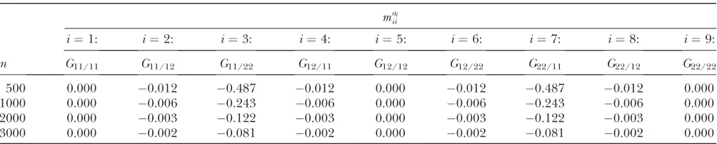
TABLE 2
Covariancesmal
ii of additive genetic sampling effects within marker classifor different numbers (n) of F2
individuals: QTL in the middle of a 10-cM marker interval
mal
ii
i¼1: i¼2: i¼3: i¼4: i¼5: i¼6: i¼7: i¼8: i¼9:
n G11/11 G11/12 G11/22 G12/11 G12/12 G12/22 G22/11 G22/12 G22/22
500 0.000 0.012 0.487 0.012 0.000 0.012 0.487 0.012 0.000
1000 0.000 0.006 0.243 0.006 0.000 0.006 0.243 0.006 0.000
2000 0.000 0.003 0.122 0.003 0.000 0.003 0.122 0.003 0.000
3000 0.000 0.002 0.081 0.002 0.000 0.002 0.081 0.002 0.000
the number of expected proportions for each marker genotype according to Equation 14. To make sure that
nl
i$1, we used n $ 500. For 500 F2 individuals this
covariancemal
ii is#1% of the QTL variance and shows a
further decline when the sample size increases. Only for marker classes G11/22 and G22/11 is there a very high
(negative) covariance (48.7% of the additive genetic variance) and an experiment with.2000 F2individuals
would be required to reach a value,10%. These marker genotypes are rare, we expect these marker genotypes to occur twice in total among 500 F2genotypes. Therefore,
omitting these covariancesmal
ii has little effect on the
likelihood.
The asymptotic variancesm˜al
ii of the additive genetic
sampling effects for different marker classes are, how-ever, larger than their corresponding covariances and, more importantly, they show considerable variation between more frequent marker classes. The sixth line of Table 3 shows the genetic sampling variances for all marker classes, again for an additive QTL in the middle of a 10-cM marker interval. For the three most frequent marker classes, the genetic sampling variance is at#1% of the additive genetic variance (classes 1, 5, and 9) and for another four marker classes it equals 25% (classes 2, 4, 6, and 8), while a 50% value occurs only in the very rare classes (3 and 7). Note that the genetic sampling variances become smaller when the QTL is located
closer to the boundary of the marker interval. The genetic sampling effects completely vanish if marker locations and positions of the QTL coincide (Table 3, first line). In such cases, the covariances of the genetic sampling effects are zero and the assumption Varð Þ ¼e Is2
eof the reduced model (16) is exact.
The latter considerations suggest, as a further alter-native, a weighted approach, where the second part of the approximation inherent in the reduced model,i.e., equal genetic sampling variances for all marker classes, is skipped, while the assumption (first part) of zero covariances for genetic sampling effects within marker class is maintained. For a single additive QTL this results in the following mixed model equations (MME):
X9WX X9W ˜Zl
˜
Z9lWX Z˜9lWZl 1V˜all
b ˜ual
¼ X˜9Wy
ZlWy
;
where l¼s2
e=s2al. The variance of the residuals is
Varð Þ ¼e Varðmal1eÞ ¼W
1s2
e, wheres2e is defined as
in (8) and all other symbols as in (1) and (16). The diagonal matrix W of order n has the entries
wss ¼s2e m˜
al
iis2al1s
2 e
1
, which differ between observa-tions from different marker classes and are equal for observations from the same marker classi. If more QTL and nonadditive genetic gene actions are considered in the model, then the genetic sampling variances for
TABLE 3
Asymptotic variancesm˜al
ii of additive genetic sampling effects within marker classifor differently sized marker intervals and different QTL positions within marker intervals (cM)
Marker interval
Position of QTL
˜ mal
ii
i¼1 i¼2 i¼3 i¼4 i¼5 i¼6 i¼7 i¼8 i¼9
0 0 0.00 0.00 0.00
10 1 0.00 0.09 0.18 0.09 0.00 0.09 0.18 0.09 0.00
10 2 0.00 0.16 0.32 0.16 0.01 0.16 0.32 0.16 0.00
10 3 0.00 0.21 0.42 0.21 0.01 0.21 0.42 0.21 0.00
10 4 0.00 0.24 0.48 0.24 0.01 0.24 0.48 0.24 0.00
10 5 0.00 0.25 0.50 0.25 0.01 0.25 0.50 0.25 0.00
20 10 0.02 0.26 0.50 0.26 0.04 0.26 0.50 0.26 0.02
30 15 0.04 0.27 0.50 0.27 0.08 0.27 0.50 0.27 0.04
40 20 0.07 0.29 0.50 0.29 0.13 0.29 0.50 0.29 0.07
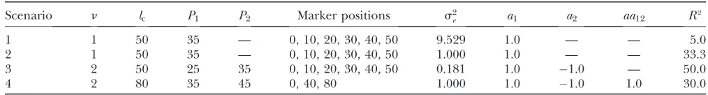
TABLE 4
Brief summary of simulated scenarios: the number of QTLn, length of the chromosomelc(cM), QTL positionsP1andP2(cM),
marker positions (cM), residual variances2
e, additive genetic effects (a1,a2), and additive-by-additive genetic effectsaa12
as well as the relative QTL varianceR2(%)
Scenario n lc P1 P2 Marker positions s2e a1 a2 aa12 R2
1 1 50 35 — 0, 10, 20, 30, 40, 50 9.529 1.0 — — 5.0
2 1 50 35 — 0, 10, 20, 30, 40, 50 1.000 1.0 — — 33.3
3 2 50 25 35 0, 10, 20, 30, 40, 50 0.181 1.0 1.0 — 50.0
different QTL and different kindstof genetic effects have to be summed to get the entire genetic sampling variance of an observation andwss(sth individual given
the marker classi) becomes
wss¼
s2
e P
t m˜ t
iis
2
t1s2e
; ð17Þ
where t 2 {al, dl, aalk, adlk, dalk, ddlk}. This weighted
version of the reduced model retains the advantage of a reduced dimension of the QTL relationship matrices as in the reduced model, but may provide a better approxi-mation of the exact residual log-likelihood-ratio test (RLRT) statistics. If marker location and position of QTL coincide, the weights of (17) are one andWis an identity matrix. The weights of (17) are similar to the weights in the weighted least-squares method of QTL mapping as shown by Xuand Atchley(1995) and Xu(1998).
Coincidence of markers and QTL results in singular-ity ofV˜al (identical toAin this case) and was not further
considered here. However, this situation can be treated,
e.g., by regularization [adding a small quantity to the diagonal elements ofV˜al (Neumaier1998)], which has
little effect on the test statistics and is easy to implement, by including allelic effects in the model instead of genotypic effects, or by replacingV˜al by a reduced rank
approximation (Ro¨ nnega˚ rd et al. 2007) obtained by
spectral decomposition.
SIMULATIONS
First, a single F2 family as the simplest case of a
combination of multiple line crosses was considered to demonstrate the properties of the reduced model in comparison to the individual model (Xie et al.1998)
and the fixed-effects methods MIM (Kao and Zeng
1997; Kao et al. 1999) and RIM (Haley and Knott
1992; Martı´nezand Curnow1992). Experiments from
four different scenarios were simulated with 1000 replications per scenario and n ¼ 200 F2 individuals
per experiment. Scenarios 1 and 2 consisted of a single additive genetic QTL at 35 cM on a single chromosome
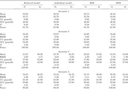
TABLE 5
Average estimates (mean) for QTL positions (P1,P2) with associated root mean squared error (RMSE) and quantiles together with
mean estimates of the residual variancesˆ2
rand the observed power (%) for different scenarios: 200 F2individuals per simulated
experiment and 1000 replications per scenario
Reduced model Individual model RIM MIM
P1 P2 P1 P2 P1 P2 P1 P2
Scenario 1
Mean 32.58 32.53 32.73 32.40
RMSE 10.71 10.79 10.78 10.89
5% quantile 9.00 9.00 9.00 9.00
95% quantile 48.00 48.00 48.00 48.00
ˆ
s2
r 9.49 9.38 9.50 9.37
Power 81.70 81.80 81.70 81.90
Scenario 2
Mean 34.82 34.87 34.88 34.68
RMSE 2.80 2.66 2.68 2.57
5% quantile 31.00 31.00 31.00 31.00
95% quantile 39.00 39.00 39.00 39.00
ˆ
s2
r 1.04 0.99 1.04 0.99
Power 100.00 100.00 100.00 100.00
Scenario 3
Mean 21.67 38.38 23.70 36.70 22.22 37.82 24.70 34.89
RMSE 4.20 4.17 2.03 2.02 4.29 4.25 1.35 1.38
5% quantile 17.00 35.00 22.00 34.00 17.00 32.00 23.00 33.00
95% quantile 25.00 42.00 26.00 38.00 28.00 42.00 27.00 37.00
ˆ
s2
r 0.27 0.18 0.28 0.19
Power 100.00 100.00 100.00 100.00
Scenario 4
Mean 34.03 46.22 33.56 46.70 34.13 46.09 32.29 44.44
RMSE 5.36 5.50 5.26 5.47 5.51 5.55 6.47 3.72
5% quantile 24.50 41.00 24.00 41.00 24.00 41.00 21.00 41.00
95% quantile 39.00 56.50 39.00 57.00 39.00 57.00 39.00 52.00
ˆ
s2
r 1.21 0.93 1.23 1.04
of 50 cM length, whereas in the other scenarios (3 and 4) there were two linked QTL with equally sized QTL effects in repulsion. In the fourth scenario chromosome length was extended to 80 cM and an interaction effect was included. For further characteristics of all scenarios see Table 4. The observations were simulated using Cockerham’s F2-metric model (Cockerham1954; Kao
and Zeng2002, Table 3). The relative QTL varianceR2
is the proportion of the phenotypic variance s2 p
ex-plained by the QTL and isR2¼s2 QTL=s2p.
In the second part our small simulation study focused on the performance of the reduced vs. the individual model in a situation with multiple families. Four inde-pendent F2families, each with 50 progeny (n¼200), were
derived from a population consisting of four different inbred lines, representing all pairwise combinations of QTL genotypes (GQQHH,GQQhh, GqqHH, Gqqhh). For each
family F1individuals were generated from a random pair
of inbred lines. Markers were always assumed to be fully informative. In the LMM family means were treated as fixed. Remaining parameters were chosen as previously described for the third scenario (Table 4). For each ge-netic effect a single (population-specific) variance was assumed. The simulated data can be found inFile S1.
Significance thresholds for the null hypothesis of no linked QTL were determined by simulating 1000 experi-ments of the same size for each scenario, where QTL with the same kind and size of effects were present, but unlinked to the markers. After analyzing these experi-ments, the 95% quantile of the maximum values of the test statistic from all replications was taken as a signifi-cance threshold, specific for each scenario and method, which allowed the determination of experimental power. We performed the residual log-likelihood-ratio test for the reduced and the individual model, the log-likelihood-ratio test for MIM, and the F-test for RIM. Mean QTL positions, root mean squared error (RMSE) of the QTL positions, and their 5% and 95% quantiles were evaluated to characterize the precision of location
estimates. For each replication we analyzed positions or combinations thereof, where marker locations and QTL positions did not coincide (step width 1 cM, both QTL in different marker intervals). Therefore, we applied RIM and MIM with the same restrictions as the VCM. Our analyses used the true genetic model for testing for segregating QTL;i.e., the model included only the simulated effects of QTL and no model selection was performed. All calculations were done with self-written Fortran 95 programs in combination with ASReml (Gilmouret al.2008) for estimation of variance
compo-nents and evaluation of the restricted maximum-likelihood function (Pattersonand Thompson1971).
DISCUSSION
Results for all simulated single-QTL scenarios are summarized in Table 5. The experimental power was 100% (scenarios 2 and 3) or nearly so (scenario 4), with the exception of scenario 1, where the experimental power was uniformly at 82% for all methods. There was almost no variation between methods in the mean estimated position in the single-QTL scenarios (1 and 2); even the distributions of the estimates showed identical 5% and 95% quantiles. Differences between methods became, however, apparent in the two-QTL scenarios. For scenario 3 (two QTL in repulsion, no interactions), MIM resulted in average estimated QTL positions at 24.7 and 34.9 cM, nearly identical to the simulated values at 25 and 35 cM. The RMSEs for positions of the QTL were,1.4 cM for both QTL for MIM and2.0 cM for the individual model, while the reduced model and RIM performed very similarly with RMSEs of4.2 cM. In scenario 3 the reduced model, the individual model, and RIM on average placed the QTL somewhat more toward the ends of the chromo-some compared to MIM and the true values, resulting in an overestimation of the distance (true distance: 10 cM) between both QTL, ranging from 2.7 cM (in-dividual model) to 6.7 cM (reduced model). For scenario 4 (two QTL in repulsion with interactions) this over-estimation of the distance between the QTL was, how-ever, very similar for all methods at 2.0–3.1 cM. The RMSEs for estimated positions of the QTL were between 5.3 and 5.6 cM with little difference between the first and second QTL for RIM as well as the reduced and the individual model. However, the RMSE of MIM at the same time showed the highest deviation of 6.5 cM for the first and the smallest deviation of 3.7 cM for the second QTL. Note that MIM was applied according to the original approach of Kaoand Zeng(1997) and Kaoet al.(1999),
which ignores double recombination events (complete interference) within the marker interval. However, double recombinations were taken into account for RIM and the VCM.
As theory indicated, estimated residual variance components from methods coping better with genetic
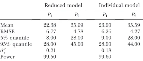
TABLE 6
Average estimates (mean) for QTL positions (P1,P2) with
associated root mean squared error (RMSE) and quantiles together with mean estimates of the residual variancesˆ2
r and the observed power (%) for the third scenario with 50 F2
individuals for each of the four families per simulated experiment (1000 replications per scenario)
Reduced model Individual model
P1 P2 P1 P2
Mean 22.38 35.99 23.00 35.59
RMSE 6.77 4.78 6.26 4.27
5% quantile 8.00 28.00 9.00 28.00 95% quantile 28.00 45.00 28.00 44.00
ˆs2
r 0.21 0.18
deviations from the mean of a marker class (MIM, individual model) were smaller in the two-QTL scenar-ios compared to RIM and the reduced model, where the genetic sampling variance (QTL genotype variability within marker genotype) is part of the residual variance. The results of the analysis of the multiple families are shown in Table 6. The accuracy of the estimated QTL positions of the individual model under consideration of four families was slightly better than that of the reduced model. However, when multiple families were considered, the difference between both models (re-duced and individual model) was less than that of the single family (scenario 3). The RMSEs for positions of the QTL as shown in Table 6 were increased compared to the RMSEs of the third scenario of Table 5, because not all families are fully informative. The observed power of the individual and the reduced model again almost reached 100%. As expected, the estimated residual variance was inflated by the within-marker genotype QTL variance.
The required CPU time for ASREML (Gilmouret al.
2008) of the reduced and the individual model was 26.7 and 80.1 sec for each repetition recorded on an HP DL380 G6 (72 GB RAM, 23XEON X5570, 2.93 GHz, multiuser environment) in a two-QTL scenario with only additive genetic effects (four families); i.e., the individual model required threefold more computing time. The run time required for the evaluation of a single QTL (scenario 1 or 2) was sevenfold for the individual model compared with the reduced model for each repetition. If the number of individuals and the number of variance components increase, the speed gain of the reduced model relative to the individual model is expected to increase.
Average RLRT profiles from the reduced and the individual model were almost identical for the first scenario with a single QTL (Figure 1A). For two QTL in scenario 3 (Figure 1B), the shapes of the RLRT surfaces from both methods were again very similar, but the average size of the maximum was higher for the individual model (60.62 compared to 44.52). The RLRT surfaces of scenario 4 of the reduced and the individual model as well as the weighted reduced model are nearly identical (results not shown). The likelihood profile of the weighted approach was smaller than that of the reduced model, but QTL positions seemed to be estimated more accurately.
The considerable advantage of the reduced model with respect to computing time is achieved by a smaller number of genetic effects accompanied by a smaller dimension of their associated covariance matrices. Moreover, this dimension does not depend on the size of the experiment, in contrast to the individual model. The amount of savable computing time can be expected to vary somewhat between different REML algorithms. Average information (AI) REML (Gilmouret al.1995;
Johnson and Thompson1995) may be implemented
either in an MME-based version or as a variant requiring the inversion of the covariance matrix Vof pheno-types, termed the ‘‘direct method’’ by Lee and Van
Der Werf (2006). These authors recommend the
direct method if genetic covariance matrices are dense because of both speed and numerical stability. Appli-cation of the Sherman–Morrison–Woodbury matrix identity (e.g., Hendersonand Searle1981; Xu1998)
to determine the inverse ofVresults in
Figure 1.—For a single QTL (scenario 1) average RLRT
V1¼ ðHGH9 1RÞ1¼R1R1H
G11H9R1H
1
H9R1;
whereRdenotes the covariance matrix of residuals,Gis the covariance matrix of all genetic effects (block diagonal), and H is the corresponding incidence matrix. To obtainV1
the inversion of a dense matrix of the same order as G is required, which usually is considerably smaller than the number of observations for the reduced model (e.g., dim(G)¼939 for a single QTL with additive genetic effects and dim(G)¼36336 for two QTL with additive genetic and dominant effects). In conclusion, the increase in computing speed obtained by the reduced model may differ between algorithms, but is substantial when compared with the individual model, thus broadening the general applica-bility of the VCM for mapping purposes.
The amount of possible improvement of the reduced model obtained by accounting for genetic sampling variation within marker classes remains to be investi-gated. A more comprehensive comparison of methods than presented here is underway to obtain a more complete picture. Despite the limited number of scenarios in our simulations, it can already be con-cluded that the proposed reduced model may be competitive with other standard methods for mapping of (multiple) QTL not only in terms of computing time, but also in terms of detection power and precision of estimated positions of the QTL.
The authors thank the reviewers for their helpful comments and suggestions. This research was supported by the German Research Foundation (Deutsche Forschungsgemeinschaft, MA 1553/3-1).
LITERATURE CITED
Abdel-Azim, G., and A. E. Freeman, 2001 A rapid method for
comput-ing the inverse of the gametic covariance matrix between relatives for a marked quantitative trait locus. Genet. Sel. Evol.33:153–173. Carbonell, E. A., T. M. Gerig, E. Balansard and M. J. Asins,
1992 Interval mapping in the analysis of nonadditive quantita-tive trait loci. Biometrics48:305–315.
Carlborg,O¨., and C. S. Haley, 2004 Epistasis: Too often neglected
in complex trait studies? Nat. Rev. Genet.5:618–625.
Cockerham, C. C., 1954 An extension of the concept of
partition-ing hereditary variance for analysis of covariances among rela-tives when epistasis is present. Genetics39:859–882.
Crepieux, S., C. Lebreton, B. Servin and G. Charmet,
2004 Quantitative trait loci (QTL) detection in multicross in-bred designs: recovering QTL identical-by-descent status infor-mation from marker data. Genetics168:1737–1749.
Gilmour, A. R., R. Thompsonand B. R. Cullis, 1995 Average
in-formation REML: an efficient algorithm for variance parameter estimation in linear mixed models. Biometrics51:1440–1450. Gilmour, A. R., B. J. Gogel, B. R. Cullis and R. Thompson,
2008 ASReml User Guide Release 3.0.VSN International, Hemel Hempstead, UK.
Grignola, F. E., I. Hoescheleand B. Tier, 1996 Mapping
quanti-tative trait loci in outcross populations via residual maximum likelihood. I. Methodology. Genet. Sel. Evol.28:479–490. Haldane, J. B. S., 1919 The combination of linkage values, and the
calculation of distances between the loci of linked factors. J. Genet.8:299–309.
Haley, C. S., and S. A. Knott, 1992 A simple regression method for
mapping quantitative trait loci in line crosses using flanking markers. Heredity69:315–324.
Haseman, J. K., and R. C. Elston, 1972 The investigation of linkage
be-tween a quantitative trait and a marker locus. Behav. Genet.2:3–19. Henderson, H. V., and S. R. Searle, 1981 On deriving the inverse
of a sum of matrices. SIAM Rev. Soc. Ind. Appl. Math.23:53–60. Jannink, J.-L., and R. Jansen, 2001 Mapping epistatic quantitative
trait loci with one-dimensional genome searches. Genetics157: 445–454.
Johnson, D. L., and R. Thompson, 1995 Restricted maximum
likeli-hood estimation of variance components for univariate animal models using sparse matrix techniques and average information. J. Dairy Sci.78:449–456.
Kao, C.-H., 2000 On the differences between maximum likelihood
and regression interval mapping in the analysis of quantitative trait loci. Genetics156:855–865.
Kao, C.-H., and Z.-B. Zeng, 1997 General formulas for obtaining the
MLEs and the asymptotic variance-covariance matrix in mapping quantitative trait loci when using the EM algorithm. Biometrics 53:653–665.
Kao, C.-H., and Z.-B. Zeng, 2002 Modeling epistasis of quantitative
trait loci using Cockerham’s model. Genetics160:1243–1261. Kao, C. H., Z. B. Zengand R. D. Teasdale, 1999 Multiple interval
mapping for quantitative trait loci. Genetics152:1203–1216. Lander, E. S., and D. Botstein, 1989 Mapping Mendelian factors
underlying quantitative traits using RFLP linkage maps. Genetics 121:185–199.
Lee, S. H., and J. H. J. Van derWerf, 2006 An efficient variance
component approach implementing an average information REML suitable for combined LD and linkage mapping with a general complex pedigree. Genet. Sel. Evol.38:25–43. Li, G., and Y. Cui, 2009 A statistical variance components framework
for mapping imprinted quantitative trait locus in experimental crosses. J. Probab. Stat.2009:1–27.
Liu, Y., G. B. Jansenand C. Y. Lin, 2002 The covariance between
rel-atives conditional on genetic markers. Genet. Sel. Evol.34:657–678. Martı´nez, O., and R. N. Curnow, 1992 Estimating the locations
and the sizes of the effects of quantitative trait loci using flanking markers. Theor. Appl. Genet.85:480–488.
Mayer, M., 2005 A comparison of regression interval mapping and
multiple interval mapping for linked QTL. Heredity94:599–605. Mayer, M., Y. Liuand G. Freyer, 2004 A simulation study on the
accuracy of position and effect estimates of linked QTL and their asymptotic standard deviations using multiple interval mapping in anF2scheme. Genet. Sel. Evol.36:455–479.
Neumaier, A., 1998 Solving ill–conditioned and singular linear
sys-tems: a tutorial on regularization. SIAM Rev. Soc. Ind. Appl. Math.40:636–666.
Patterson, H. D., and R. Thompson, 1971 Recovery of inter-block
in-formation when block sizes are unequal. Biometrika58:545–554. Ro¨ nnega˚ rd, L., K. Mischenko, S. Holmgren and O¨ . Carlborg,
2007 Increasing the efficiency of variance component quantita-tive trait loci analysis by using reduced-rank identity-by-descent matrices. Genetics176:1935–1938.
Ro¨ nnega˚ rd, L., R. Pong-Wongand O¨ . Carlborg, 2008 Defining
the assumptions underlying modeling of epistatic QTL using var-iance component methods. J. Hered.99:421–425.
Smith, S. P., 1984 Dominance Relationship Matrix and Inverse for an
In-bred Population.Mimeo, Department of Dairy Science, Ohio State University, Columbus, OH.
Wang, T., R. L. Fernando, S.van derBeek, M. Grossmanand J. A.
M.vanArendonk, 1995 Covariance between relatives for a
marked quantitative trait locus. Genet. Sel. Evol.27:251–274. Xie, C., D. D. Gesslerand S. Xu, 1998 Combining different line
crosses for mapping quantitative trait loci using the identical by descent-based variance component method. Genetics149:1139– 1146.
Xu, S., 1996 Mapping quantitative trait loci using four-way crosses.
Genet. Res.68:175–181.
Xu, S., 1998 Mapping quantitative trait loci using multiple families
of line crosses. Genetics148:517–524.
Xu, S., and W. R. Atchley, 1995 A random model approach to
inter-val mapping of quantitative trait loci. Genetics141:1189–1197.
GENETICS
Supporting Information
http://www.genetics.org/cgi/content/full/genetics.110.122333/DC1
Complex Genetic Effects in Quantitative Trait Locus Identification:
A Computationally Tractable Random Model for
Use in F
2Populations
Daisy Zimmer, Manfred Mayer and Norbert Reinsch
D. Zimmer et al.
2 SI
FILE S1
Supporting Data
File S1 is available for download as a compressed file at http://www.genetics.org/cgi/content/full/genetics.110.122333/DC1. The folder contains:
ReadMe.pdf