ABSTRACT
WANGWATCHARAKUL, WORAWUT. Modeling Inventory Systems with Imperfect Supply. (Under the direction of Russell E. King and Donald P. Warsing.)
We study inventory systems operating under an infinite-horizon, periodic-review base-stock control policy with stochastic demand and imperfect (i.e., less than 100% reliable) supply. We model demand using a general discrete distribution and replenishment lead time using a geometric distribution, resulting from a Bernoulli trial-based model of supply uncertainty. We develop a computational approach using a discrete time Markov process (DTMP) model to minimize the total system cost and obtain the optimal base-stock level when the backorder penalty is given. We develop a general, recursive solution for the steady state probability of each inventory level and use this to find the optimal base-stock level in this setting. Moreover, for specific demand distributions we are able to develop closed-form solutions for these outcomes.
The lead-time demand (LTD) distribution can also be obtained from these recursive equations to determine the base-stock level when a target customer service level is specified in lieu of a backorder penalty cost. We conduct extensive computational experiments to observe the robustness of various approximate solutions under two scenarios for the lead-time distribution. The first scenario assumes a geometric lead lead-time. The second scenario considers a general lead-time distribution. We conduct computational experiments to observe the conditions in which the DTMP model performs well, including situations where the demand and the lead-time distributions are specified separately, and where the LTD distribution is given and follows either a Beta distribution or a bimodal distribution.
Modeling Inventory Systems with Imperfect Supply
by
Worawut Wangwatcharakul
A dissertation submitted to the Graduate Faculty of North Carolina State University
In partial fulfillment of the requirements for the Degree of
Doctor of Philosophy
Industrial and Systems Engineering
Raleigh, North Carolina 2009
APPROVED BY:
_______________________________ ______________________________ Dr. Russell E. King Dr. Donald P. Warsing
Chair of Advisory Committee Co-Chair of Advisory Committee
ii
DEDICATION
iii
BIOGRAPHY
iv
ACKNOWLEDGEMENTS
I would like to express my sincere gratitude to my advisor and co-advisor, Dr. Russell King and Dr. Donald Warsing for their invaluable guidance, constant support, and kindness. I have gained considerable knowledge and improved my academic skills throughout the
v
TABLE OF CONTENTS
LIST OF TABLES…………... ix
LIST OF FIGURES………. x
CHAPTER 1 Introduction and motivation……….1
References……… 5
CHAPTER 2 OPTIMAL BASE-STOCK LEVELS FOR AN INVENTORY SYSTEM WITH IMPERFECT SUPPLY……… 6
1. Introduction……….. 6
2. Model………. 10
2.1 Model specification………..10
2.2 Analytical results for general discrete demand distribution……….13
2.2.1 Explicit forms of the steady state probability distribution ……... 13
2.2.2 Solution procedure……… 14
2.2.3 Decomposition of the total cost……….17
2.2.4 Performance measure of the system and its bounds………. 19
2.3 Analytical results for specific demand distributions………20
2.3.1 Closed-form solutions: EOQ-type customer………20
2.3.2 Closed-form solutions: Geometric demand………. 22
vi
3. Model with service level constraint………... 26
3.1 A procedure to determine a service-constrained optimal base-stock level……….. 26
3.2 Application to lead-time demand distribution………. 27
3.3 Numerical example……….. 30
4. Conclusions……… 32
References……….. 34
Appendices……….36
CHAPTER 3 COMPUTING BASE-STOCK LEVELS FROM APPROXIMATE LEAD-TIME- DEMAND DISTRIBUTIONS UNDER IMPERFECT SUPPLY……… 43
1. Introduction……… 43
2. Markov model and analysis………... 45
2.1 Model characteristic………. 45
2.2 Service- level model and service performance measures………. 48
2.3 Effect of changing penalty cost and target service level on the total system cost... 50
3. Comparing approximation methods under geometric lead time……… 51
3.1 Approximation methods……….. 53
3.2 Experiment results………54
4. Comparing approximation methods under general lead time……… 56
4.1 Demand and lead-time distributions specified ………56
4.1.1 Data………. 57
4.1.2 LTD distribution parameters………... 58
4.1.3 Experimental results………61
vii
4.2.1 Symmetric beta distribution……… 64
4.2.2 Right-skewed beta distribution……… 65
4.2.3 Left-skewed beta distribution……….. 66
4.2.4 Bimodal lead-time demand distribution………...67
5. Conclusions……… 67
References……….. 69
Appendices……….71
CHAPTER 4 COMPUTING BASE-STOCK LEVELS FOR A SERIAL INVENTORY SYSTEM WITH IMPERFECT SUPPLY……….. 78
1. Introduction………... 79
2. Model………... 80
2.1 Model specification…..……….80
2.2 System dynamics……….. 82
2.3 Computing transition probabilities………85
2.4 Numerical experiments………. 86
2.4.1 Impact of h2 on the optimal base-stock levels………... 88
2.4.2 Impact of αon the optimal base-stock levels………... 89
2.4.3 Impact of b1 on the optimal base-stock levels………... 89
3. Decentralized approximation methods………...90
3.1 Method1: Functional form of implied backorder pe nalty………. 91
3.2 Method 2: Decentralized objective function………. 94
4. Experimental results………...96
5. Conclusions……….…... 98
viii
Appendices………...102
CHAPTER 5
ix
LIST OF TABLES
CHAPTER 3
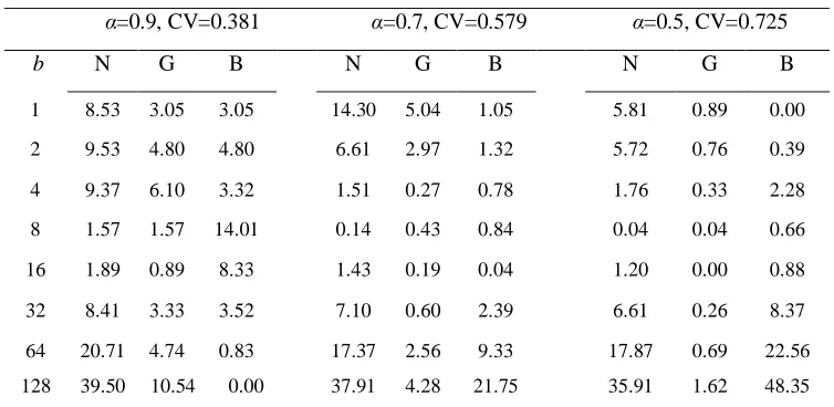
Table 1. Deviation (%) from optimal cost of approximation methods
for Poisson demand ………..…… 55
Table 2. CV of LTD for all combinations of demand and lead time distributions ……... 58
Table 3. Average deviation (%) from optimal cost, symmetric LTD ………... 64
Table 4. Average deviation (%) from optimal cost, right-skewed LTD ………... 65
Table 5. Average deviation (%) from optimal cost, left-skewed LTD ………... 66
Table 6. Average deviation (%) from optimal cost, bimodal LTD ………...67
CHAPTER 4 Table 1. Summary of demand parameters used in this experiment………... 87
Table 2. Summary of cost deviation from optimal (expressed as %) for method 1 for different demand parameters………... 94
Table 3. Summary of cost deviation from optimal (expressed as %) for method 2 for different demand parameters………... 96
Table 4. Beta demand distributions used in the experiment……….. 97
x
LIST OF FIGURES
CHAPTER 2
Fig. 1. The sequence of events during period t………... 12 Fig. 2. Inventory cost vs. base-stock level when α=0.9,h=1,b=20……….18 Fig. 3. Inventory cost vs. base-stock level: α = 0.9 for different ratios of b/h ………….. 18 Fig. 4. δ(α) vs α ………...………….. 24 Fig. 5. Rate of change on cost deviation vs. b for different demand distributions ……... 25 Fig. 6. DTMP-derived LTD distribution for different demand distributions
and supply risk factors………... 28 Fig. 7. Comparing the base-stock level from three methods………. 31
CHAPTER 3
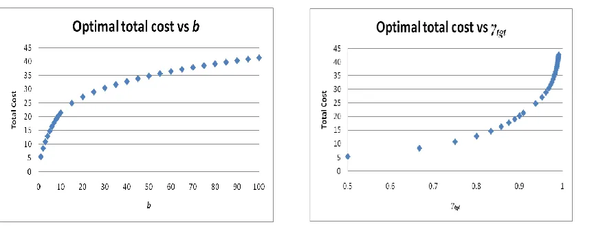
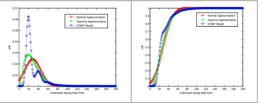
Fig. 1. LTD distribution for different demand distributions and supply risk factors…….48 Fig. 2. Optimal total cost vs backorder penalty and target service level……….. .51 Fig. 3. Comparisons of the pdf and cdf of LTD distribution for various methods ……... 52 Fig. 4. The relationship between optimal base-stock and optimal total cost
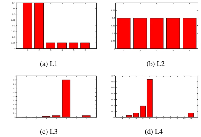
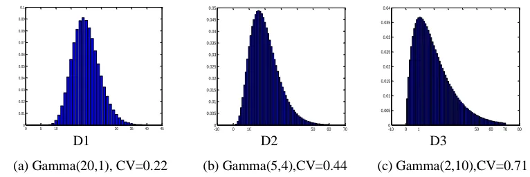
for different CV of X ……… 52 Fig. 5. Lead-time distributions used in computational experiments……….. 57 Fig. 6. Gamma demand distribution used in computational experiments……….. 58 Fig. 7. Comparative resluts across six different approximation models
for the D2-L4 case …... 62 Fig. 8. Bimodal distributions generated from Poisson distributions
xi
CHAPTER 4
Fig.1. System configuration………... 80
Fig.2. Sequence of events during a period………. 82
Fig.3. Different beta demand distributions……… 87
Fig.4. Optimal base-stock levels vs. h2, when b1 = 20, α = 0.85………88
Fig.5. Optimal base-stock levels vs. α, when h2 = .5, b1= 20……… 89
Fig.6. Optimal base-stock levels vs. b1, when h2 = .5, α = 0.85……….90
Fig.7. Optimal node 2 penalty cost vs. Fitted node 2 penalty cost………... .92
Fig.8. Total system cost for decentralized system vs. b2……….. 95
1
CHAPTER 1
Introduction and motivation
In this dissertation, we study an inventory system operating under a periodic-review, base-stock control policy with stochastic demand and imperfect (i.e., less than 100% reliable) supply. Under imperfect supply, a constant nominal lead time for re-supply becomes a
stochastic replenishment time, with an obvious impact on the system’s ability to meet a specified customer service level. Two basic approaches to determine optimal base-stock levels are the ―shortage costing approach‖ and the ―service-level approach,‖ the latter applying to the case for which the shortage penalty cost is not specified (Dullaert et al., 2007). We develop a computational approach to obtain the optimal base-stock level for the shortage-costing case, and also show that the method can be modified to handle the service-level case. For specific demand distributions, we are able to develop closed-form solutions for the optimal base-stock level, and we also develop expressions for upper and lower bounds on the corresponding optimal service level. To handle the service-level case, traditional methods for computing base-stock levels require the distribution of demand during the lead time be specified. When demand and lead time are stochastic, however, analytically tractable forms of the lead-time demand (LTD) distribution can be obtained from the convolution of two distributions of demand and lead time, which is viable for only few special cases. An approximation method which assumes the LTD distribution is Normally distributed has been widely used to estimate the base-stock level with central limit theorem justification (e.g., Tyworth and O’Neill, 1997). We examine the accuracy of this and several other
approximation methods under both restricted and general lead time cases to observe the practical value of our model.
2
using a geometric distribution resulting from a Bernoulli trial-based model of supply uncertainty. A discrete-time Markov process model (DTMP) is used to minimize the total system cost, comprised of inventory holding and backorder penalty costs. We present two complementary scenarios. In the first scenario, when penalty cost is specified, we develop a general, recursive solution for the steady state probability of each inventory level and use this to find the optimal base-stock level in this setting. Moreover, for specific demand
distributions we are able to develop closed-form solutions for these outcomes, and we also develop expressions for upper and lower bounds on the corresponding optimal service level. We also quantify the impact of supply risk on the deviation from the optimal cost under fully reliable supply. In the second scenario, when the penalty cost is not known, we seek a base-stock level that satisfies a service-level target. This setting also assumes demand and lead time conditions that result in a variety of lead-time demand shapes. We compare the base-stock levels from our DTMP model with a model that uses the traditional assumption of Normally-distributed demand and lead time. We find that the Normal approximation consistently overestimates the optimal base-stock level up to a threshold service level, and beyond that, underestimates it, clearly based on the bimodal nature of LTD. Not only does our method generate base stock levels that more accurately determine the optimal base stock, but it is also much more flexible in that it can accommodate any discrete demand
distribution.
3
corresponding backorder penalty, resulting from the specified service level that makes the two models equivalent. The functional relationship between a required service level and optimal total cost is investigated to observe the effect of the service level target on the total system cost.
We conduct extensive computational experiments to observe the robustness of various approximate solutions under two scenarios depending on the lead-time distribution. The first case is based upon assumptions of a geometric lead time and a discrete demand distribution, such that the DTMP model represents the real system. We investigate the quality of three approximations to the DTMP model: Normal and gamma approximations that match the first two moments of the LTD distribution, and a statistical bootstrap procedure that uses a re-sampling approach to approximate the LTD. In the second set of experiments, we consider a general situation where the lead time is not restricted to a geometric distribution. To investigate the practical value of the DTMP model, we treat it as an alternative
approximation to a simulated near-optimal base-stock level. The model parameters are estimated by matching the first two or three moments with the ones from data sampled from the true, underlying LTD distribution (Lau, 1989). We perform numerical experiments where the demand distribution and the lead-time distribution are modeled individually, and when the LTD distribution is characterized by a discretized beta distribution or a bimodal
distribution. The cost deviations from the simulation results are compared in both cases. In addition, we observe the conditions when the model provides a good approximation, and the influence of changing coefficient of variation of the LTD on cost deviation.
4
building block of this two-node serial system. Since a closed-form solution appears to be unattainable, direct numerical computation is a viable approach to finding an optimal solution. When the state space of this model increases, however, computational complexity becomes an issue. In order to reduce the search space and computational time, we develop two approximation methods to find a good starting solution. The decomposition-based
5
REFERENCES
Chopra. S., Reinhardt. G., & Dada. M. (2004). The effect of lead-time uncertainty on safety stocks. Decision Sciences, 35(1), 1–24.
Dullaert, W., Vernimmen, B., Aghezzaf, E., & Raa, B. (2007). Revisiting service-level measurement for an inventory system with different transport modes. Transport Reviews, 27(3), 273-283.
Lau, H.S. (1989). Toward an inventory control system under non-normal demand and lead-time uncertainty. Journal of Business Logistics, 10, 89–103.
6
CHAPTER 2
Optimal Base-stock Levels for an Inventory System with
Imperfect Supply
Abstract
We develop a method to compute the optimal base-stock level under supply and demand uncertainty for an infinite-horizon, periodic-review inventory model. A discrete-time Markov process (DTMP) model is used to minimize the total system cost, comprised of inventory holding and backorder penalty costs. We present two complementary scenarios. In the first scenario, when penalty cost is specified, we model demand using a general discrete distribution and replenishment lead time using a geometric distribution, resulting from a Bernoulli trial-based model of supply uncertainty. We develop a general, recursive solution for the steady state probability of each inventory level and use this to find the optimal base-stock level in this setting. Moreover, for specific demand distributions we are able to develop closed-form solutions for these outcomes, and we also develop expressions for upper and lower bounds on the corresponding optimal service level. We quantify the impact of the level of supply uncertainty on the deviation from the optimal cost under fully reliable supply, and In the second scenario, when the penalty cost is not known, we seek a base-stock level that satisfies a service-level target. This setting also assumes demand and lead-time conditions that result in a bimodal lead-time demand distribution. In this setting, we compare the base-stock levels from our DTMP model with a model that uses the traditional assumption of Normally-distributed demand and lead time. We find that the Normal approximation consistently overestimates the optimal base-stock level up to a threshold service level, beyond which it underestimates it, which appears to be driven by the bimodal nature of lead-time demand. Not only does our method generate base stock levels that accurately determine the optimal base stock, but it is also flexible in that it can accommodate any discrete demand distribution.
1.
Introduction
7
stochastic demand and imperfect (i.e., less than 100% reliable) supply. Periodic review is practical, easy to implement, and suitable for an inventory system of a single, fast-moving product or multiple independent products transported jointly from a single supplier. The base-stock inventory control policy is widely used in practice since it is easy to implement in a periodic replenishment framework and has been proven to be optimal when set up cost is negligible (Clark and Scarf, 1960). In our model, the nominal replenishment lead time is one period, with a Bernoulli trial probability of α that the quantity on-order is filled in that one-period lead time. Under these conditions, the replenishment lead time follows a geometric distribution with parameter α. We formulate a discrete-time Markov process (DTMP) model with a finite state space to determine the optimal base-stock level in this single-site inventory system. The total cost for this system is comprised of inventory holding and backorder penalty costs. This DTMP model can be viewed an extension of the classical newsvendor model in an infinite-horizon setting with the risk of a supply shortfall. Intuitively, more inventory needs to be carried to hedge against supply uncertainty. Our goal is to provide an approach to compute the optimal base-stock level that accounts for this supply uncertainty in addition to the uncertainty in demand. We also extend our analysis to determine the base-stock level required to satisfy a service level target in the case for which a backorder penalty is not specified.
In academic research, it is typical to assume Normally distributed demand and lead-time distributions, owing to the simplicity of convolving two Normal distributions to specify the resulting lead-time demand (LTD) distribution. The use of the Normal distribution to model customer demand is questionable in many situations, though, especially when the coefficient of variation is high. Also, a symmetric lead time distribution is difficult to justify in a realistic setting. These issues motivate us to establish a computational approach or approximation procedure to assist a decision maker in managing inventory in a timely manner under rapidly changing environment such as facing dynamic period demand
8
the lead time falls in a fairly narrow range of values, possibly a multimodal distribution in the case of supply disruptions that irregularly result in long lead times.
We present two complementary scenarios. In the first scenario, when the backorder penalty cost is given, the model allows determination of the optimal base-stock level and the corresponding optimal service level to minimize the total system cost. For some specific demand distributions, a closed-form expression for the optimal base-stock level is developed, based on the steady state probability of inventory levels. We use these expressions to specify upper and lower bounds on the optimal service level. In the second scenario, where the backorder penalty cost is not known but a service level target is specified, we formulate a model to determine the base-stock level to meet this customer service level based on the approach developed for the first scenario. The LTD distribution clearly plays a key role in determining a base-stock level, safety stock, or reorder point to meet a required service level. The derivation of the LTD distribution using the convolution of demand and lead-time distribution is, however, a challenging task in general and may be possible only for particular lead time and demand distribution pairs. When lead time is deterministic, it is easy to
compute the LTD distribution. When lead time is stochastic, however, the Normal
approximation is extensively used to estimate the LTD distribution and the base-stock level. A distribution-free method using a convex combination of discrete lead-time probability is another approach for safety stock and reorder point determination (Tyworth and O’Neill, 1997). The DTMP model here provides the exact solution and can incorporate any discrete demand distribution and resulting LTD distribution from underlying supply interruption.
9
sporadic and not necessarily symmetric (Tersine, 1988). Moreover, the compound Poisson is generally used when a demand batches of random size occur at random inter-arrival times.
Random supply interruptions are the consequence of a diversity of situations, including equipment breakdowns, material shortages, strikes, natural disaster, and political crises (Mohebbi, 2003). The random nature of supply uncertainty has been modeled in several ways to characterize the replenishment lead time such as on/off rates. In this continuous-review framework, the status of the supply process is typically modeled as ―on‖ (available) and ―off‖ (unavailable) states. Transitions between these two states are typically modeled as a continuous-time Markov process to exploit the memoryless property. Arreola-Risa and De Croix (1998) use an on/off rate model to provide optimal values of (s,S) policy parameters including optimal inventory strategy with different severity of supply disruptions with partial backorder. They use a more general stockout behavior, that is, the unfilled demands become a mixture of lost sales and backorders. Gupta (1996) studies the impact of an unreliable supplier on the operating cost in a continuous review (s,Q) system. The supplier on-off periods follow an exponential distribution. Parlar and Perry (1995) incorporate two unreliable suppliers in an (s,Q) model with independent non-identical on/off periods following exponential distribution. In this paper, the inventory is reviewed periodically.
Lead time is another significant stochastic element in an inventory system. A common simplifying assumption is a constant or zero lead time due to the complexity of solving a more general system analytically. Mohebbi (2003) generalizes the (s,Q) inventory model of Gupta (1997) by allowing Erlang (Ek) distributed lead times and exponentially
distributed on-off periods and provides an analytical cost-minimization model in a lost-sales environment. Mohebbi (2004) provides an exact expression of the long-run average cost rate function by extending the model in Mohebbi (2003) to incorporate a hyperexponentially-distributed lead time. He employs an alternating renewal process to model the supplier availability where the on and off periods follow general and hyperexponential distributions, respectively. In this study, we concentrate on how inventory is affected by underlying
10
In our study, we conduct numerical experiments to capture model behavior under different model parameters. The results from this single-node model allow us to gain some managerial insights and serve as a building block for considering a set of base-stock levels in more complex system configurations in multi-node supply chains such as serial systems or assembly or distribution networks.
2.
Model
2.1.Model specification
Our model assumes a periodic-review inventory system with negligible fixed ordering costs. This implies that a base-stock policy is optimal (Clark and Scarf, 1960). At the
beginning of each period, an order is made to the supplier to bring the inventory position back up to the base-stock level. However, the supplier is not entirely reliable. Here, we assume that the re-supply process in each period is a Bernoulli trial, meaning that with probability αthe supplier delivers the current order and any accumulated backorders at the end of the current period (without capacity constraint, independent of the order size). If the nominal lead time is one period, then the supply uncertainty induces a stochastic
replenishment lead time having a geometric distribution with parameter α. The customer demand in our model is i.i.d. over time, following a given discrete (or discretized) non-negative distribution. The backorder penalty cost is incurred per unit of backordered demand in any period when the demand is not fulfilled and the on-hand inventory level is negative.
11
for the optimal base-stock level, the corresponding service level, and the optimal holding and backorder costs as a function of the model input parameters.
The following notation is used to describe the model. S = base-stock level
S* =optimal base-stock level g = maximum backorder level
Ω = state space of the system = g,..., 1, 0,1,...,S It = on-hand inventory at the end of time t (It )
α = probability that the total quantity on-order arrives in the current period Dt = customer demand in period t (assumed stationary)
P
d t
p D d for d dmin, ,dmax (dmin 0 and dmax ) h = holding cost per unit per period
b = backorder penalty cost per unit per period
πi = steady-state probability of being in state i, where i = end-of-period on-hand
inventory
[ ]i max( , 0)i
[ ]i max( , 0)i BC = backorder cost
IC = inventory holding cost
During any period t in the infinite horizon, three events determine the state transition. Each of these events is described below and their timing is displayed in Figure 1.
1. An order is placed to bring the inventory position back up to the base-stock level S. 2. With probability α, supply arrives from the order in step 1 including any unfulfilled
12
3. Customer demand is observed and fulfilled, up to the current inventory level. The state of the system is evaluated at this point in time.
Note that the demand is accumulated over the whole period and filled at the time of event 3. Also, the supplier incurs the inventory holding cost during the transportation. When the order arrives (event 2), the holding cost is incurred immediately after the replenishment of the customer orders (event 3).
Event
Timing
t
t
1
t
t
1
1
2,3
Period
Fig. 1. The sequence of events during period t
The objective is to minimize the long-run total system cost which consists of inventory holding cost and backorder penalty cost. The cost parameters, both holding and backorder penalty, are assumed to be stationary and independent of the current state. The decision variable is the base-stock level S. Specifically, the objective function is
Minimize ( ) i
i
TC S h i b i
Here πi is a function of demand uncertainty (i.e., the demand distribution) and supply
13
2.2.Analytical results for general discrete demand distribution
In this section, we assume demand each period follows some arbitrary discrete distribution. On-hand inventory is subject to uncertainty in supply and is given by
It 1 max g , It y S It Dt 1 ,
where y 0 w.p. 1 and y 1 w.p. .
2.2.1. Explicit forms of the steady state probability distribution
The probability of transitioning from state i to state j in a period is 1
[ ]
ij P It j It i . The state-transition probability matrix, P [ ij], is constructed based
on the supply uncertainty parameter α and demand mass function (pd ). Given the base stock
level, S, and the maximum backlog, g, the size of the P matrix is S g 1 S g 1 . Since we concentrate on a finite number of states, g is arbitrarily assigned to the system, but chosen carefully the steady state probability of state g is reasonably close to 0.
Assume that the current state is i (It i). If the supplier is able to ship, then after satisfying customer demand It 1 S S, 1,S 2, ,S dmax with probabilities p0, p1, andp2,…,
max
d
p , respectively. On the other hand, if the supplier is unable to ship, then
1 , 1, 2, , 1 ,
t
I i i i g g with probabilitiesp0, p1, p2,…, pg 1, d
d g p ,
respectively. Based upon this, the state transition probabilities are
0
1 1
0 0
(1 ) (1 )
[1 ] (1 )[1 ]
S j
S j
ij i j S j
S g i g
k k
k k
p i j
p p i j
p p i j g
14
Based on the particular operating characteristics of the system, the steady-state probability vector can be derived without explicitly solving the system of linear equations. Under steady-state conditions, P . The right-most column of the P matrix is used to obtain
0 1 1 0
S p g g S p S,
which yields
0 0
1 (1 )
S
p
p (1)
We can use expression (1) to solve the remaining column-wise terms of the system P , ultimately yielding a recursive expression,
1 1 1 max 0 (1 )
1, 2, ,
1 (1 )
d
d d k s k
k S d
p p
d d
p (2)
As we show in subsequent section, for some special cases of the demand distribution, we can derive a closed-form solution of the steady state distribution of the DTMP.
2.2.2. Solution procedure
A procedure to find the base-stock level to minimize the total system cost starts from considering the objective function with respect to the base-stock level S, specifically
TC( ) i
i
i i
i i
S h i b i
hi h b i
h b i bi
15
Proposition 1: The objective function TC(S) is aconvex function of S. Proof.
TC(S) is convex if and only if the second difference of the function is non-negative for all S. The second difference of TC(S) is
2
TC TC 2 2TC 1 TC( )
TC 2 TC 1 TC 1 TC .
J J J J
J J J J
Substituting into the expression for TC(S), above, we obtain 1
2
0 0
1
TC
( ) ,
J J
S d S d
d d
S J
J b b h b b h
b h
which, by definition, is non-negative.
Proposition 2: Base-stock level S is optimal if
1
0 0
and .
S S
S d S d
d d
b b
b h b h
Proof.
The difference of total cost of two adjacent base-stock levels, TC(J), is used to obtain the optimal base-stock level. For any non-negative integer J,
1 1 1 2 3
TC J h JpS J 1 pS pS J b pS J 2pS J 3pS J
and therefore,
1 2 3 4
16
Computing the first difference,
0 1
0 0
0 TC( ) TC( 1) TC( )
1
( ) .
J
S d S d
d d J
J J
S d S d
d d
J
S d d
J J J h b
h b
b b h
Since 0
J
S d d
is monotonically non-decreasing in J and the objective function is convex, the
optimal base-stock level S* can be found as the first value that results in the first positive value of TC(J). In other words, the optimal solution can be characterized using a critical fractile approach. Therefore, S is an optimal base-stock level if
0 S S d d b
b h and
1 0 . S S d d b b h
The convexity of the objective function and the optimal condition in Proposition 2 can be used to develop a procedure to find the optimal base-stock level (S*), as follows:
1. Calculate the steady-state probabilities from the recursive equations (1) and(2).
2. S* is given by
*
0,1,2, 0
arg min :
J S d
J d
b
S J
b h .
From these results, we observe the following:
1. The above procedure can be applied to any discrete demand distribution with non-negative values.
2. The components of the vector π S, S 1, , g are independent of the
17
Given the above observations, if we know pd and α, we can compute the optimal base-stock level by comparing the summation of steady-state probabilities with a ratio of system costs b and h. Moreover, we can state the following proposition.
Proposition 3: If 0
S
S d d
b
b h , there is a pair of optimal base-stock levels, S and S+1. Proof:
From the proof of Proposition 2, we know that the difference of total cost of two adjacent base-stock levels S and S+1 is
0
TC( 1) TC( ) ( )
S
S d d
S S b b h .
If 0
S
S d d
b
b h, then by Proposition 2,
*
S S is an optimal base-stock level, but the first-difference expression above also implies that TC(S 1) TC( )S 0, meaning that
TC(S 1) TC( )S , meaning in turn that both S and S 1 are optimal.
2.2.3. Decomposition of the total cost
18
10 20 30 40 50 60 70 80 90 100
0 50 100 150 200 250
S : (base-stock level)
T o ta lc o s t
Total Cost(TC) vs Base-stock level(S)
Total cost Inventory holding cost Backordering cost
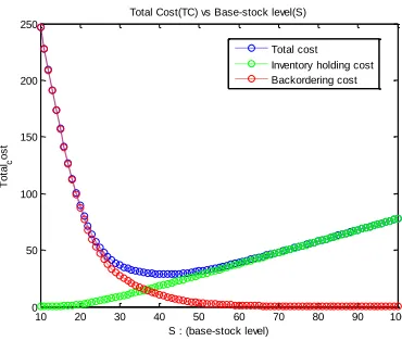
Fig. 2. Inventory cost vs. base-stock level when 0.9 , h 1, and b 20 The inventory holding cost monotonically increases with the base-stock level. In contrast, the backordering cost monotonically decreases with the base-stock level. Thus, the total cost must be convex in S as depicted in Figure 2. As shown in Proposition 2, the
optimal base-stock level depends mainly on the cost ratio, b/h. Figure 3 exhibits the shape of total cost for several values of cost ratio (b/h). The larger the cost ratio (b/h), the larger the minimum point on the total cost curve, and therefore the larger the optimal base-stock level (S*).
0 20 40 60 80 100 120
0 100 200 300 400 500 600 700 800 900
Total Cost vs Base-stock for different cost ratio b/h
Base-stock T o ta l C o s t b/h=10 b/h=30 b/h=50 b/h=70
19
2.2.4. Performance measure of the system and its bounds
We define the service level, γ, as the probability of not stocking out in any period. When a stockout occurs, the on-hand inventory at the end of the period is negative.
Therefore, the summation of all non-negative states after the demand fulfillment determines the service level (i.e., the probability of non-negative stock) for the system, specifically * * * 0 S S d d ,
where S* is the optimal base-stock level and * is the corresponding optimal service level.
From Proposition 2,
* * 0 S S d d
b b h . Thus, a lower bound on the optimal service level
is * b b h . As stated in Proposition 3, if 0
S S d
d b b h , there are two optimal
base-stock levels, S and S+1. Nevertheless, base-stock level S+1 has a service level at least as high as, if not higher than, that of base-stock level S. From Proposition 2,
*
0
S S d
d b b h and
*
1 0
S S d
d b b h . An upper bound on the optimal service
level is therefore
min, , max
max S d
d d d
b b h . From equation (2), max{ S d}
d ≤ max{d pd}
for any demand distribution and α. Hence, a more readily computed upper bound is *
min 1, max( d)
d b
p
b h .
20
Hence, α has less impact on γ*when the backorder penalty is high, irrespective of the
demand distribution. Moreover, the upper and lower bounds of γ*are tighter when the CV of the demand distribution is large or where max( d)
d p is comparatively low. 2.3.Analytical results for specific demand distributions
For the general demand distribution case, the steady state probability distribution of the inventory level is determined by recursive equations (1) and (2). The optimal base-stock level is obtained from the simple procedure described in Section 2.2.2 above. However, for some specific demand distributions, we are able to derive closed-form solutions for the steady state probability, the optimal base-stock level, the corresponding optimal service level and the holding and backorder costs of the system.
2.3.1. Closed-form solutions: EOQ-type customer
In this section, we consider an intermittent and lumpy demand pattern. In a business-to-business setting, the customer demand distribution may actually be the result of an
ordering policy. Here we assume the customer ordering policy is of EOQ-type. Specifically, at the end of each period the customer evaluates its inventory position and if it is below its system reorder point, the customer places a replenishment order for q units. Since the EOQ-type policy generates a fixed order quantity, the customer order would be either exactly q units or zero in each period. Customer demand is therefore discretely distributed with non-zero p0 and pq, i.e., a (q,0) demand distribution, such that
0 0
0 w.p.
w.p. , 1.
t
q q
p D
q p p p .
Based on the recursive equations of the steady-state probability in the general case, the long-run probability of each level of on-hand inventory can be expressed as
21
0 0 1 max 1 0 for
1 (1 )
(1 )
for ; 1, 2, ,
1 (1 )
0 otherwise. d d q i d p i S p p
i S qd d d
p
Based on the explicit form of the steady state probabilities, and using the procedure to find the optimal base-stock level in the general case, the closed-form solution for the optimal base-stock level is
2 0 *
log 1 (1 )
log( )
q p
b A
a
b h A p
S q
a ,
where A 1 (1 )p0and a (1 )pq A. The derivation is shown in Appendix B.
When the optimal base-stock level S* is known, the optimal service level γ* is represented as a function of the demand probabilities andthe supply uncertainty factor α, yielding
* 0 (1 )
(1 ) 1
n
p a a
A A a ,
where n S q* and A and a are defined as above.
The decomposition of the total cost in section 2.2.3 shows that the optimal base-stock level balances the inventory holding and backorder costs. Similarly, closed-form expressions for holding and backorder costs can be computed as functions of S,α, p0 and pq, yielding
* 1
0
2
(1 ) (1 ) (1 )
(1 ) 1 (1 ) (1 )
n n n
S p S a a q a a na a
IC h
A A a A a
22
1
2 2
(1 )
,
(1 )
n n q n
bq p
BC
A a
where A and a are as defined above. The following properties can be observed from the expressions derived above. It is
obvious from the closed-form expression that the optimal base-stock level is always an integer multiple of q as determined by the input parameters. We observe the impact of each parameter independently by holding all other parameters fixed. The results are consistent with our intuition. That is, the optimal base-stock level is high when α is low, pq p0 is high, and b h is high. However, α has more influence on the optimal base-stock level as pq p0 increases. As the value of α decreases, however, the cost ratio b h has a more pronounced impact on the optimal base-stock level. The graphs from these experiments are shown in Appendix C.
2.3.2. Closed-form solutions: Geometric demand
In this section, we observe the system behavior when the customer demand follows a geometric distribution, Dt Geo(p), meaning that 1 , 0,1, , max
d d
p p p d d .
Closed-form solutions can be obtained for the steady state probability distribution, optimal base-stock level, optimal service level, and optimal inventory holding and backorder costs.
Based on the recursive equations of the steady-state probability in the general case, the long-run probability of each level of on-hand inventory can be expressed as
1 max
(1 )
0,1, ,
1 (1 )
d
S d d
p p
d d
p
23
Based on the explicit form of steady state probabilities, and using the procedure to find the optimal stock level in the general case, the closed-form solution for the optimal base-stock level is
2 *
log 1 (1 )
(1 ) log( )
b p A
a
b h A p p
S
a ,
where A 1 (1 ) p and a 1 p A. The derivation is shown in Appendix D. The corresponding optimal service level is
* 1
* (1 )
1
S
p a
A a .
Closed-form expressions for holding and backorder costs can be computed as functions of S,α, p0 and pq, yielding
1 1
2
(1 ) (1 ) (1 )
1 (1 )
S S S
hp a a a a Sa
IC S
A a a
and 1 2 (1 ) S bpa BC
A a .
2.4 Effect of changing supply risk on the total system cost
24
* *
1 *
1
( ) ( )
( ) , 0 1
( )
TC S TC S
TC S . (3)
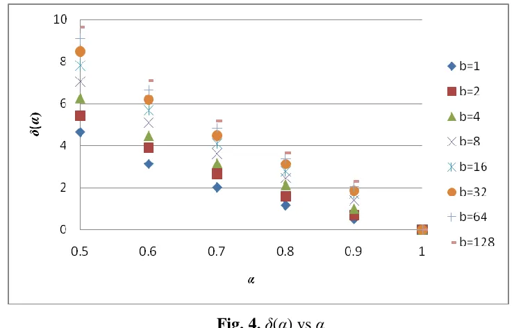
We observe that the functional form of the relationship is consistent across different demand distributions and mean values. Figure 4 depicts this functional relationship for different backorder penalty costs (b) when demand follows a Poisson distribution with λ=20.
Fig. 4. δ(α) vs α
For a practical range of α values,0.5 1, it appears that is linear. For b=16, for example, a linear regression yields 14.89 14.94 , with R2
98.67% and the linearity test shows a p-value of 0.000042. From this regression equation, therefore, a decrease of α by 0.01 increases the cost deviation from the perfect-supply case by 0.1494, or approximately 15%. By manipulating equation (3), the total system cost can also be
expressed in terms of the total system cost under fully reliable supply as
25
where m is the slope of the linear regression line. In this case, for example,
* *
0.9 1
TC S 2.49 TC S and * *
0.8 1
TC S 3.99 TC S .
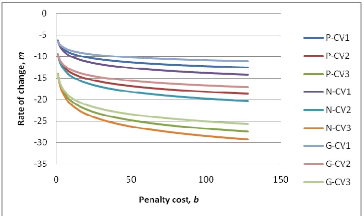
However, the rate of change of the cost deviation—i.e., the slope m of the linear regression equation between and α—depends on the penalty cost and the demand
distribution. Figure 5 depicts the regression relationship between b, m, and CV for different demand distributions—Poisson, Normal, and Gamma.
Fig. 5. Rate of change on cost deviation vs. b for different demand distributions where P=Poisson demand, N=Normal demand, G=Gamma demand
and CV1=0.316, CV2=0.223, CV3=0.158.
26
m ( 21.04 0.31 48 CV) ( 4.2 1.475 7.98 CV) ln( )b . (5)
Thus, we can approximate the total system cost—through a combination of expressions (4) and (5)—as a function of the total system cost under fully reliable supply when the CV and skewness of the period demand are known for a specified value of backorder penalty cost.
3.
Model with service level constraint
In the previous model, we assume that the backorder penalty cost is given, and therefore that the optimal base-stock level can be computed directly in a way that accounts for the demand and supply uncertainty parameters. Based on the optimal base-stock level, the corresponding optimal customer service level can be determined. In some situations, the objective is to meet or exceed a customer service target at minimum total system cost. Thus, a minimum customer service level constraint is specified. In such situations, the previous model can be modified to satisfy a service level constraint by minimizing only the inventory holding cost. This model is more realistic because it is often difficult to determine a
reasonable backorder penalty cost. In this section, we develop a computational approach to determine the base-stock level to satisfy a given service level.
3.1.A procedure to determine a service-constrained optimal base-stock level
27
1. Calculate the steady-state probabilities from the recursive equations (1) and(2). 2. Find the smallest non-negative value of S such that is at least equal to the target
service level ( tgt), i.e.,
*
tgt 0,1,2, 0
arg min :
S
S d
S d
S S .
The procedure above is optimal for any discrete demand distribution with
geometrically distributed lead time. Below, we compare our method with classical methods that rely on the LTD distribution to determine the safety stock and order-up-to level in a system subject to demand and lead-time uncertainties.
3.2.Application to lead-time demand distribution
The probability of demand during lead time being equal to d units can be
28
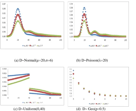
Fig. 6. DTMP-derived LTD distribution for different demand distributions and supply risk factors.
To determine the base-stock level or order-up-to level to meet a target customer service level under arbitrary or unspecified demand and lead-time distributions, a common approach is to assume that the LTD is Normally distributed (Lau and Lau, 2003). Another approach is to use a convex-combination of the conditional probability distribution of demand for each discrete lead-time value (Tyworth and O’Neill, 1997). The more general approach that specifies the LTD distribution from the convolution of the demand and lead-time distributions is analytically tractable for only few special cases. Using the Central Limit
(a) D~Normal(µ=20,σ=6) (b) D~Poisson(λ=20)
29
Theorem as justification, other researchers have used a Normal distribution to approximate the LTD distribution and compute base-stock levels (e.g., Tyworth and O’Neill, 1997).
The effectiveness of using a Normal distribution to approximate the LTD distribution has been an active area of debate in the inventory literature. Some authors, such as Eppen and Martin (1988), have questioned the effectiveness of the Normal approximation. They reveal the errors in estimating the probability of stocking outusing the Normal
approximation to determine the safety stock level. Similarly, Chopra et al. (2004), demonstrate that Normal approximation can lead to poorly specified inventory levels, especially when the CV of period demand is high or when the lead time follows a skewed (e.g., gamma) distribution. These errors could lead to misleading managerial insights regarding how to specify buffers to guard against the combined effects of demand and lead-time uncertainty. On the other hand, Tyworth and O’Neill (1997) conduct empirical
experiments to examine the robustness of the Normal approximation of the LTD distribution for fast-moving products in seven major industries. They conclude that the Normal
approximation is robust with respect to logistics system cost, total costs, and fill rate. Based on the overview found in Tyworth and O’Neill (1997) we describe the various approximations of LTD that we use in our computational comparison below. Where
appropriate, we retain the notation developed in Section 2 above, with additional notation as follows:
X = Lead-time demand random variable µX = Mean of LTD distribution
σX = Standard deviation of LTD distribution
µD = Mean per-period demand;
max
min
d
D d d pd d
σD = Standard deviation of per-period demand:
max
min
2 2
d
D d d pd d D
L = Lead-time random variable
T = Set of lead-time values, t T and Pt P L t
µL = Mean lead time (periods)
σL = Standard deviation of the lead time (periods)
30
Normal approximation: Assume that LTD X is Normally distributed. The mean and standard deviation of X can be obtained from the first two moments of demand and lead time, and the base-stock level to meet a required service level can be calculated as follows:
X D L
X D2 L2 L D2
Sˆ X k X, where
1 tgt
k and is the standard normal cdf.
Convex combination of conditional probability: This is a distribution-free method, with no assumption required for the shape of the convolution of the demand and lead-time distributions. The procedure was developed by Bank and Fabrycky (1987) and Eppen and Martin (1988). It uses a convex combination of the conditional probability distributions of demand during the discrete values of lead time. However, its use is restricted to the cases where the period demand distribution is Poisson, Gamma, Normal, or Exponential. When demand is Normally distributed and lead time is discrete, the base-stock level to meet a specific service level can be calculated as follows:
X Dt t D, t T
X Dt t D, t T
tgt
0,1,2,
ˆ min : P
t t
t T S
S S P D S .
3.3.Numerical example
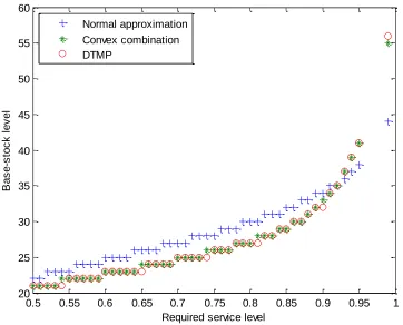
We compare the approaches discussed above with the DTMP model, under the restriction that demand has a discrete distribution and lead time has a geometric distribution. A discretized Normal distribution is utilized to represent the customer demand and truncated at 0 and µ+5σ. Figure 7 shows the resulting base-stock levels for the three methods for the case with µ = 20, σ = 6, and a nominal lead time of one period with supply risk factor α = 0.9.
31
0.5 0.55 0.6 0.65 0.7 0.75 0.8 0.85 0.9 0.95 1
20 25 30 35 40 45 50 55 60
Required service level
B
a
s
e
-s
to
c
k
l
e
v
e
l
Normal approximation Convex combination DTMP
Fig. 7. Comparing the base-stock level from three methods— D 20, D 6,
and L Geo 0.9
For this system, the replenishment lead time has a geometric distribution, and therefore the DTMP model generates the optimal base-stock level for each required service level. The computed base-stock levels in Figure 5 are similar to the ones from the convex combination method with some slight deviations. The Normal approximation method
overestimates the base-stock levels at low target service levels until a value of approximately 0.92, after which it underestimates the optimal base-stock level.
For these experimental conditions, with geometric lead time and discretized Normal demand, the DTMP model provides the optimal base-stock level. The DTMP model is, however, also advantageous when demand is not Normally distributed since it can
32
not geometrically distributed, the effectiveness of the DTMP model to approximate the base-stock level is a question we address in follow-on research.
4.
Conclusions
We propose a single-location inventory model under supply uncertainty. The model operates under base-stock control in a periodic-review framework. The supply uncertainty is modeled as a Bernoulli trial, with a specified probability α that the total quantity on-order is fulfilled at the end of the current period. The nominal lead time is one period. The
replenishment lead time therefore follows a geometric distribution with parameter α. Thus, our model can be viewed as an extension of the newsvendor model with supply risk. A discrete-time Markov process (DTMP) model is introduced to solve the problem analytically. The steady state distribution of the on-hand inventory can be calculated from recursive equations given the demand distribution parameters and α. We find that a critical fractile approach may be used to obtain the base-stock level that minimizes the total system cost. For some specific demand distributions, we are able to compute the optimal base-stock level—and the optimal service level and total system cost—in closed-form. We also provide upper and lower bounds on the corresponding optimal service level γ*. Empirical analysis indicates that α has less impact on γ*when the backorder penalty cost is high, irrespective of the demand distribution, and that the upper and lower bounds on γ* are tighter when the coefficient of variation of the demand is large. We quantify the impact of the supply uncertainty on the cost deviation from the optimal cost under fully reliable supply. We also present an approximate logarithmic relationship between the rate of change on the cost deviation and the penalty cost.
33
convolve generally specified lead time and demand distributions. A popular approximate method is to assume a Normally distributed LTD distribution. Our approach, however, is to modify our first (DTMP) model to compute the optimal base-stock level. Our analysis shows that a Normal approximation to the base-stock level can deviate significantly from the optimal result across a wide range of target service levels.
The results from this single-site inventory model allow us to gain important
34
REFERENCES
Arreola-Risa, A. and DeCroix, G. A. (1998). Inventory management under random supply disruptions and partial backorders. Naval Research Logistics, 45(7), 687-703.
Banks J. and Fabrycky W. J.( 1987). Procurement and inventory systems analysis (Englewood Cliffs, N.J.: Prentice-Hall, 129-139.
Chopra, S., Reinhardt, G., and Dada, M. (2004). The effect of lead-time uncertainty on safety stocks. Decision Sciences, 35(1), 1–24.
Clark, A. J. and Scarf, H. (1960). Optimal policies for a multi-echelon inventory problem. Management Science, 6, 475–490.
Eppen, G. D. and Martin, R. K. (1988). Determining safety stock in the presence of stochastic lead-timeand demand. Management Science, 34(11), 1380-1390.
Gallego,G. and Özer, Ö. (2005). A new algorithm and a new heuristic for serial supply
systems. Operations Research Letters, 33(4), 349-362.
Gupta, D. (1996). The (Q,r) inventory system with an unreliable supplier. INFOR, 34(2), 59-76.
Lau, H. S., and Lau, A. H. L. (2003). Nonrobustness of the normal approximation of lead-time demand in a (Q, R) system. Naval Research Logistics, 50(2), 149-166.
Mohebbi, E. (2003). Supply interruptions in a lost-sales inventory system with random lead-time. Computers and Operations Research, 30(3), 411-426.
35
Parlar, M. (1997). Continuous-review inventory problem with random supply interruptions. European Journal of Operational Research, 99(2), 366-385.
Parlar, M. and Perry D. (1995). Optimal (Q, r, T) policies in deterministic and random yield models with uncertain future supply. European Journal of Operational Research,84, 431– 443.
Sherbrooke, C. (2004). Optimal inventory modeling of systems: multi-echelon techniques, second ed. Springer-Verlag, New York, LLC.
Tersine, R. J. (1988). Principles of inventory and materials management, New York: North-Holland.
Tomlin B. (2006). On the value of mitigation and contingency strategies for managing supply chain disruption risks. Management Science, 52(5), 639-657.
36
37
APPENDIX A
Impact of demand distribution, backorder penalty cost and α on optimal service levels
Poisson (λ=20), CV=0.224 Uniform (0,40), CV =0.577
38
APPENDIX B
Derivation of optimal base-stock level for (q,0) discrete demand distribution
From Proposition 2, base-stock level S is optimal if
1
0 0
and .
S S
S d S d
d d
b b
b h b h
Let S* be the optimal base-stock with S*= nq where n is a positive integer
Therefore, * 0 S S d d b b h
Let A 1 (1 )p0 and substituting S d from the closed-form expression (2)
1 0 1 1 2 1 0 2 (1 )
(1 ) (1 ) (1 )
1 ... d d n q d d n
q q q q
p
p b
A A b h
p p p p
p b
A A A A A b h
Given a (1 )pq
A and substituting into the above yields
0 2 2 0 2 0 2 0 2 0 1 1 1 1 (1 ) 1 (1 ) 1 (1 ) log 1 log( ) n q n q n q n q q p
p a b
A A a b h
p
a b A
a b h A p
p
b a A
a
b h A p
p
b a A
a
b h A p
p
b a A
n a
b h A p
39
2 0
log 1 (1 )
log( )
q p
b A
a
b h A p
n
a
Since, from Proposition 2,
* 1
0
S
S d d
b b h, S
*
is the first value of S that satisfies the inequality and n is the smallest integer that satisfies the inequality above, therefore
2 0 *
log 1 (1 )
log( )
q p
b A
a
b h A p
S q
40
APPENDIX C
Impact of system parameters on optimal base-stock levels
Optimal base-stock level vs. pq /p0 Optimal base-stock level vs. α
41
APPENDIX D
Derivation of optimal base-stock level for geometric demand
From Proposition 2, base-stock level S is optimal if
1
0 0
and .
S S
S d S d
d d
b b
b h b h
Let S* be the optimal base-stock
* 0 S S d d b b h
Let A 1 (1 ) p and substituting S d from the closed-form expression (2)
* * * 1 1 2 1
2 2 1
(1 )
(1 ) (1 ) (1 ) (1 )
[1 ... ]
d S d d S S
p p p b
A A b h
p p p p p p b
A A A A A b h
Given a 1 p
A and substituting into the above yields
* * * * 2 2 2 2 2 *
(1 ) 1 1 1
1 (1 )
(1 ) 1 (1 ) (1 ) 1 (1 ) (1 ) [log( )] log 1
(1 )
S
S
S
S
p p p a b
A A a b h
a b p A
a b h A p p
b p a A
a
b h A p p
b p a A
a
b h A p p
b p a A
S a
b h A p p
42
2 *
log 1 (1 )
(1 ) log( )
b p A
a
b h A p p
S
43
CHAPTER 3
Computing Base-stock Levels from Approximate Lead-time
Demand Distributions under Imperfect Supply
Abstract
We consider an infinite-horizon, periodic-review, inventory model under a base-stock control policy and supply uncertainty. A discrete-time Markov process (DTMP) model is used to obtain the optimal base-stock level when the backorder penalty and inventory holding costs are given. Under these assumptions, the lead-time demand (LTD) distribution can be obtained from recursive equations. This distribution is significant in determining the base-stock level to satisfy a target service level. We conduct experiments to observe the quality of various approximate solutions under two scenarios, when lead time has a geometric distribution and when lead time has any distribution. In the first scenario, we observe the quality of the classical approximations of LTD, Normal and gamma distributions, approximating the optimal base-stock level by matching the first two moments of the LTD distribution obtained from the DTMP model. In the second scenario, we consider a general situation where the lead-time distribution is not restricted to a geometric distribution, and simulation is used to generate the LTD distribution. In this case, the DTMP model is used as an alternative LTD approximation to determine the base-stock level that meets the target service level. We perform experiments where the demand distribution and the lead-time distribution are specified individually, and where the LTD distribution is specified by a discretized beta distribution or a bimodal distribution. We assess the quality of the approximate solutions by computing their cost deviations from the simulation results.