Models for Optimizing Resource Allocation in a Cancer Center.

(1)

ABSTRACT

WOODALL, JONATHAN C. Models for Optimizing Resource Allocation in a Cancer Center. (Under the direction of Dr. Brian Denton.)

Cancer centers are the central hub of the health care system for most cancer patients. Patients visit to receive consultations with their oncologists and treatment. Medical advances and an aging population have resulted in patient volumes steadily increasing over time, a trend that is expected to continue. Some studies indicate a simultaneous increase in demand and potential decrease in the supply of nurses, which has created pressure on healthcare managers and administrators to improve efficiency of oncology services. Process improvements could help improve patient access and at the same time increase revenue to providers. Additional potential benefits include a more predictable, manageable, and evenly distributed workload for employees, as well as reduced waiting times for patients. This thesis focuses on the development and validation of a discrete event simulation model for a large medical center. We discuss the most important aspects of cancer center operations, the model building and validation process, and we provide examples of several research questions related to predicting bottlenecks in a cancer center and designing monthly, daily, and weekly nurse schedules.

(2)

(3)

(4)

Models for Optimizing Resource Allocation in a Cancer Center

by

Jonathan C. Woodall

A thesis submitted to the Graduate Faculty of North Carolina State University

in partial fulfillment of the requirements for the Degree of

Master of Science

Industrial Engineering

Raleigh, North Carolina 2011

APPROVED BY:

_________________________ _________________________ Dr. James Wilson Dr. Russell King

______________________________ Dr. Brian Denton

(5)

BIOGRAPHY

Jonathan was born in Orlando, Florida, where he spent much of his childhood. He and his family moved to Raleigh, NC, shortly before he started high school, where he currently lives. Jonathan received his B.S. in Industrial Engineering from NC State University in December 2009, graduating with Magna Cum Laude honors.

Jonathan recently spoke at the INFORMS Healthcare conference in Montreal, Canada, presenting much of this thesis work. Professionally, Jonathan has had several internships over his time in college, interning with Progress Energy and the Duke Medical Center, working with process development and analysis. Jonathan has also been involved with simulation projects through NC State, working with UNC Chapel Hill and the Mayo Clinic on simulation projects. He recently began working a full-time job at Duke Medicine as a management engineer.

(6)

ACKNOWLEDGEMENTS

A huge thank you is really a small token of appreciation for Dr. Brian Denton, my advisor on this project. He has been very much an encourager, friend, and motivator all the way through the project. His guidance has helped to constantly challenge me to grow and improve my skills. Many thanks go to Michael Murr, a student who has helped to run many of the experiments for the cancer center. Thanks go to Dr. James Wilson and Dr. Stephen Roberts, whose expertise and knowledge of discrete event simulation were very helpful in working on this thesis. Other thanks go to the many professors and students who have helped me learn and grow both as a student and a professional along the way, including Dr. Russell King, Dr. Javad Taheri, Dr. Tom Reiland, Dr. Tom Culbreth, and Bjorn Berg, who has been a constant encourager, supporter, and sounding board for any ideas and questions I have had along the way.

Many thanks also go to those at Duke Medical Center that have made this project and been very supportive of my work since day one, including Tracy Gosselin, Chad Seastrunk, Bill Fulkerson, Amy Boswell, Celia Walsh, Craig Johnson, Steve Power, and Nancy Hedrick, all of who have provided expertise and input along the way. Many thanks to the pharmacy staff for allowing me to do so many time studies and to the treatment center nursing staff for their input and patience in educating me about the various processes.

This thesis was funded by the Duke Cancer Institute. I appreciate their funding of this project, which has led to me accepting a full time position at Duke Medicine working in the Performance Services Department. I appreciate the support Duke has shown me in finishing up my education and helping me grow as a professional.

(7)

LIST OF TABLES

Table 3.1: Arrivals per hour calculations for each time block in a clinic on Thursday. ... 28

Table 3.2: List of probability distributions and their sources as used in the simulation model (all times in minutes). ... 32

Table 3.3: List of routing percentages and their sources as used in the simulation model. ... 33

Table 3.4: Processes analyzed for fitting without data; parameter estimates and distribution fit based on expert opinion (minutes where applicable for time units). ... 36

Table 3.5: Comparison of simulation arrivals with system data for validation. ... 40

Table 3.6: Results for flow time values in each of the clinics of the model over each day of the week. ... 42

Table 3.7: OTC flow times by treatment type for the OTC-only simulation model. ... 43

Table 3.8: OTC waiting room time values. ... 44

Table 3.9: Wait time results in the clinic portion of the model. ... 46

Table 3.10: OTC waiting room time results for the OTC-only model. ... 47

Table 3.11: Patient waiting time for different resources in the OTC-only model. ... 49

Table 4.1: Different PT nurse shifts considered in the MIP monthly scheduling model. ... 61

Table 4.2: Expected throughput values and anticipated off-service volume for each DBG. ... 62

Table 4.3: Daily nursing hour requirements for each DBG for every day of the week. ... 63

Table 4.4: Nurse staff level and shift policy combinations for daily schedule optimization. ... 68

(10)

Table 4.6: Potential shift times for OTC nurses under differing shift lengths. ... 69

Table 4.7: Expected daily throughput for each DBG in the OTC. ... 69

Table 4.8: Sample schedule of nurses for the HOA DBG. ... 71

Table 4.9: Sample capacity schedule for each time block of the day for an HOA DBG nurse schedule. ... 74

Table 4.10: MIP results for the optimal allotment of nurses, 21 FTE scenario. ... 75

Table 4.11: Results of 21 nurse simulation-optimization comparing original and optimal schedules. ... 80

Table 5.1: Different numbers of chairs used to test bottlenecking in the OTC for each day. ... 87

Table 5.2: Results for the numbers of chairs at which each day has no chair wait. ... 91

Table 5.3: Results for Increasing Patient Arrivals on Wednesday in the new OTC. ... 92

Table A2.1: Patient arrival and volume information for the surgical oncology clinic. ... 110

Table A2.2: Patient arrival and volume information for the hematology oncology clinic. ... 111

Table A2.3: Patient arrival and volume information for the brain tumor center. ... 112

Table A2.4: Patient arrival and volume information for the prostate center. ... 113

Table A2.5: Patient arrival and volume information, direct OTC arrivals. ... 114

Table A2.6: Patient arrival and volume information for all OTC arrivals regardless of clinic. ... 115

Table A3.1: Random variable describing the allotment of scheduled infusion length as a discrete 5-point distribution. ... 119

Table A4.1: Nurse schedules in the OTC in the base case representing the current OTC. ... 120

(11)

Table A4.3: PSA Capacity Schedules (Check-in and Check-out for Clinics). ... 122

Table A4.4: Capacity schedules for OTC receptionists. ... 123

Table A4.5: Capacity schedules in the pharmacy. ... 123

Table A4.6: List of all resources in the simulation model with fixed capacity levels. ... 124

Table A5.1: All 10-hour shift candidate schedule – 21 total nurses. ... 126

Table A5.2: Mix of 10-hour and 8-hour shift candidate schedule – 21 total nurses. ... 126

Table A6.1: Results from MIP for 18 nurse staffing level scenario. ... 131

Table A6.2: Results from MIP for 16 nurse staffing level scenario. ... 132

Table A6.3: PT nurse selection, 21 nurse scenario. ... 133

(12)

Table A6.7: Average and maximum wait room time comparison, original vs. optimizer, 18 nurses.

... 135

Table A6.8: Average and maximum wait room time comparison, original vs. optimizer, 16 nurses. ... 136

Table A6.9: All 10-hour shift optimizer schedule, 21 nurse scenario. ... 137

Table A6.10: Mix of 10-hour and 8-hour shift optimizer schedule, 21 nurse scenario. ... 137

Table A7.1: Results for different wait times as numbers of chairs change on Monday. ... 143

Table A7.2: Results for different wait times as numbers of chairs change on Tuesday. ... 144

Table A7.3: Results for different wait times as numbers of chairs change on Wednesday. ... 145

Table A7.4: Results for different wait times as numbers of chairs change on Thursday. ... 146

Table A7.5: Results for different wait times as numbers of chairs change on Friday. ... 147

Table A8.1: Monday results for the new-OTC model with patient volume increases. ... 153

(13)

(14)

LIST OF FIGURES

Figure 2.1: Diagram of total patient throughput by day in the treatment center. ... 7

Figure 2.2: Average daily throughput numbers in the treatment center by day of week. Bars indicate 95% Confidence Intervals. ... 8

Figure 2.3: Percentage breakdown of the source of patients in the treatment center. ... 10

Figure 2.4: Pie Chart showing the punctuality of treatment center arrivals. ... 11

Figure 2.5: Analysis of average number of patient arrivals in the treatment center by time of day for a given day of the week. ... 12

Figure 3.1: Flow chart showing the high-level patient flow through the cancer center. ... 18

Figure 3.2: Flow Chart of the major steps in the clinic patient flow process. ... 20

Figure 3.3: Flow chart of treatment center process prior to treatment being initiated. ... 21

Figure 3.4: Flow Chart of treatment center flow process following treatment. ... 22

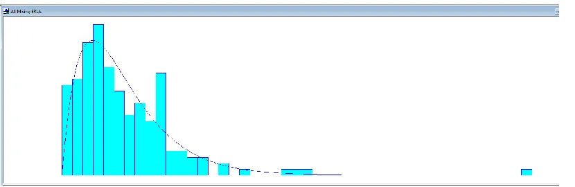
Figure 3.5: An example of an Erlang Probability Distribution Fit for Drug Mixing Process (1.5 + ERLA(2.94,2)). ... 35

Figure 3.6: Graph from simulation model run showing the number in queue for chairs and nurses in the OTC. ... 50

Figure 4.1: Diagram illustrating relationship between major components in OTC nurse scheduling... ... 55

Figure 4.2: Best objective function values (shortage hours) for MIP runs, 21 nurses. ... 77

Figure 4.3: Best objective function values (shortage hours) for MIP runs, 18 nurses. ... 77

(15)

Figure 5.1: Patient wait times for chairs with respect to the number of chairs on Thursday. ... 89

Figure 5.2: Patient wait times for nurses with respect to the numbers of chairs on Thursday. ... 89

Figure 5.3: Patient waiting room time with respect to the number of chairs on Thursday. ... 90

Figure A1.1: Punctuality for Surgical Oncology Clinic. ... 106

Figure A1.2: Punctuality for Hematology Oncology Clinic. ... 107

Figure A1.3: Punctuality for Brain Tumor Center. ... 107

Figure A1.4: Punctuality for Prostate Center. ... 108

Figure A3.1: % Clinic Patients with Port Draws: 5 + 13*BETA(2.26, 2.46); sqaure error = 0.007541.. ... 116

Figure A3.2: Drawn to Receive Labs Time (Lab Processing): 9.5 + GAMM(12, 1.33); square error = 0.000954. ... 117

Figure A3.3: Lab Received to Verified (Lab Processing): 19.5 + LOGN(19.5, 35.7); square error = 0.001898. ... 117

Figure A3.4: Pharmacist Processing Time: -0.5 + LOGN(5.46, 6.74); square error: 0.010918. ... 117

Figure A3.5: Technician Mix Drug (Pharmacy): 1.5 + ERLA(2.94, 2); square error = 0.006274. ... 118

Figure A3.6: Radiology Processing Time: 30 + GAMM(62.2, 1.18); square error = 0.000569. ... 118

Figure A3.7: Check-out Hematology Oncology: LOGN(9.33, 11.3); square error = 0.007150. ... 118

Figure A7.1: Patient wait for chairs graph, Monday. ... 148

Figure A7.2: Patient wait for nurses graph, Monday. ... 149

Figure A7.3: Patient waiting room time, Monday. ... 149

(16)

Figure A7.5: Patient wait for nurses graph, Tuesday. ... 150

Figure A7.6: Patient waiting room time, Tuesday. ... 150

Figure A7.7: Patient wait for chairs graph, Wednesday. ... 150

Figure A7.8: Patient wait for nurses graph, Wednesday. ... 151

Figure A7.9: Patient waiting room time, Wednesday. ... 151

Figure A7.10: Patient wait for chairs graph, Friday. ... 151

Figure A7.11: Patient wait for nurses graph, Friday. ... 152

(17)

(18)

Recent years have seen many medical advances, particularly in the area of heart disease. These advances have resulted in fewer patients dying of heart disease, and overall increase in life expectancy. However, as a consequence of these improvements, there have been increases in the likelihood of cancer diagnosis over the course of a patient’s lifetime. In many countries cancer is, or is rapidly becoming, the leading cause of death. As a result, patient demand for cancer center services has been steadily increasing, and is expected to continue to increase (Erikson et al., 2007). Furthermore, this is expected to lead to significant shortage in oncology.

Cancer centers are the central hub of the health care system for most cancer patients. Patients attend cancer centers to receive consultations with their oncologists and treatment for cancer. Increasing patient demand has created patient and staff scheduling challenges. From the patient perspective, high demand often results in long waiting times. This can be in the form of direct waiting (waiting on site to see a provider or receive treatment) or indirect waiting (waiting for a scheduled appointment). From the staffing perspective, high demand results in higher resource utilization, and congestion that can be frustrating for providers. In a high-demand environment, variation in patient mix can result in portions of the cancer center, or parts of the day, being overloaded, while other areas, or times of day, are underutilized. From the provider perspective, process improvement can allow for more patient throughput, and thus more revenue. It can also mean less stress for employees (and ultimately lower turnover) as the workload becomes more evenly distributed, predictable, and manageable. Therefore, process improvements can help bridge the gap between supply and demand for oncology services. Furthermore, reduced waiting time is associated with more timely treatment, which may result in improved health for patients served by the cancer center.

(19)

involves many different resources and processes, each with differing amounts of variation, and the potential to be a bottleneck in the overall process.

In this thesis we use quantitative models to investigate ways to improve the efficiency of a cancer center. The main focus of this thesis is on the development of a validated simulation model at a cancer center. The model is used to forecast the success of potential process improvements. This predictive ability allows decision-makers the ability to systematically look at many potential alternatives for improvement and identify the best route for improvement. Furthermore, the simulation model is used to recommend design decisions for a new cancer center, and to predict the effect of resource allocation decisions prior to the use of the new cancer center.

Our simulation model was built to represent a particular cancer center at a large academic medical center. However, the insights we draw from our study are applicable to other cancer centers. We begin by describing a conceptual model of a cancer center. Next, we describe the various parts of the discrete event simulation model, development of a non-stationary Poisson arrival process to represent the randomness and unpredictability of patient arrivals, methods for fitting input distributions of process variability, and validation of the model. The model combines the interaction of multiple clinics, the oncology treatment center (OTC), central labs, radiology (where scans are performed for patients), and the pharmacy. Furthermore, it includes complexities of all the various employees responsible for caring for patients along with their work schedules.

(20)

The simulation model is also used to evaluate two planning scenarios for a new hypothetical cancer center. We conduct a series of experiments using the simulation model for predictive purposes to determine likely bottlenecks in the new cancer center, and to be used for contingency planning with regard to design decisions and nurse staffing and scheduling decisions.

(21)

(22)

Section 1: Overview of Cancer Center Operations

Patients visit cancer centers for many reasons such as referrals from primary care physicians due to suspicion of cancer, second opinions, consultation on treatment type and location, check-up consultations while undergoing treatment, and follow-up consultations upon completion of treatment. The location in which patients visit doctors is called the clinic. Most cancer centers have clinics organized based on type of cancer (e.g. breast, prostate, lung). A second major part of a cancer center is the treatment center, or OTC. The OTC is the location in which patients who have been diagnosed with cancer receive chemotherapy treatment. The goal of chemotherapy is to attempt to cause the cancer to go into remission. Chemotherapy can be received in the form of an injection or an infusion, where medicine is dripped intravenously into the patient (referred to as an IV). Patients may also receive radiation treatment for their cancer, though hospitals vary on whether this location is near or far from the OTC.

There are additional locations in the cancer center that play key roles. One is radiology, the location in which radiation imaging scans are performed. Another is the location of the central labs, where patient blood tests and other lab tests are processed. Most patients who receive chemotherapy or a consultation with an oncologist must have blood drawn. Blood counts are an important part of diagnosis, and they must be reviewed prior to receiving chemotherapy. This can pose a constraint on patient flow through the cancer center, as treatment cannot start until the blood draw has been processed by the lab, and the patient is deemed able to receive the specified treatment.

(23)

Section 2: Data Analysis and Barriers to Efficient Patient Flow

The large number of interacting areas of the cancer center, and natural variation in the time to complete activities creates a large amount of uncertainty and variability in the patient flow process. As mentioned, there are also challenges posed by a steady increase in patient demand for cancer center services. Figure 2.1 below illustrates the increase in patient volume seen in the OTC over the time from which all arrival data in the model came specifically. A linear trend line has been added to illustrate the increase in patient volume over the time period. The combination of increasing demand for cancer center services and a large number of interacting areas in the cancer center creates significant challenges in managing patient flow. Therefore, it is of particular interest to cancer center management to examine how to best to reduce the negative impacts of this uncertainty. While our data does not cover the span of an entire year, and thus may not capture seasonality in patient arrivals, expert opinion of OTC administration staff has indicated that patient volume has steadily increased over time. For example, July 2009 had less volume than July 2010, and each corresponding month as well.

Figure 2.1: Diagram of total patient throughput by day in the treatment center. 60

70 80 90 100 110 120 130 140

Thr

ou

ghp

ut

(24)

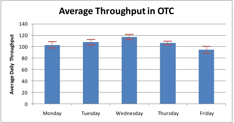
Patient arrivals vary depending upon day of week. For example, Figure 2.2 below shows the average throughput in the oncology OTC for each day of the week, with 95% confidence intervals noted by the red bars based on historical arrival data from the time period of July-October 2010. The graph shows some variation across weekdays, with Wednesday being the busiest day, and Friday being the least busy day. The difference in average expected throughput from Wednesday to Friday is approximately 20 patients. This day-to-day variation further complicates planning and resource allocation decisions. The variation in daily demand at the OTC is largely driven by the clinic arrivals in the cancer center. Clinic arrivals are in turn driven by the days in which oncologists practice in clinic. This day-to-day variation in OTC patient volumes is also consistent with expert opinion, and is the case year-round, as patient volume is driven by oncologist availability rather than demand for services, since in this case, the demand far exceeds the supply.

Figure 2.2: Average daily throughput numbers in the treatment center by day of week. Bars indicate 95% Confidence Intervals.

Patient flow patterns in the cancer center differ depending upon the type of patient. In general, a patient receiving treatment will start at one of the clinics, have labs drawn and processed, and will finish at the OTC. However, patients may be classified in several different ways. For

0 20 40 60 80 100 120 140

Monday Tuesday Wednesday Thursday Friday

A

ve

ra

ge

D

ai

ly

T

hr

ou

ghp

ut

(25)

instance, some patients visit the cancer center only for a clinic visit. Of the patients solely receiving a clinic visit, some will have labs and/or radiology, others will not. Some patients are return visits and some are new visits; new visits tend to have longer service times in the clinic. Some patients may go from the clinic to the OTC on the same day, while others may return on a different day for treatment. This variation in patient flow further contributes to uncertainty in resource utilization from day to day.

Of the patients arriving to the OTC, some arrive after visiting other portions of the cancer center and others arrive directly. However, all patients receiving treatment must have their blood drawn to verify they are healthy enough to receive the chemotherapy. Since all blood specimens must be taken within 24 hours of treatment, patients arriving directly must either have had labs drawn the day before at an approved off-site location or must visit one of the labs in the cancer center to have their blood drawn. If review of the blood work indicates patients are not healthy enough to receive treatment, their physician is contacted either to approve the treatment or change the regimen (strength and type of drug) used. Upon receiving treatment, patients generally leave the facility, although they may occasionally have to visit radiology or the clinic afterwards.

Figure 2.3 below illustrates the wide variety of types of patient flow and classifications within the cancer center. The pie chart shows the varying sources of arrivals into the OTC. The largest contributors to OTC throughput are the surgical oncology and hematology oncology clinics, as well as the independent arrivals formed by the collection of scattered arrivals from other clinics in the hospital or direct into treatment. These arrivals do not require a clinic visit, but require labs on or off-site within 24 hours of treatment. Bottlenecks in source clinics can significantly affect the process flow of patients into the OTC. Surgical oncology and hematology oncology are important in particular as they supply such a large percentage of the patient volume.

(26)

patients arrive within 30 minutes of the scheduled time. Therefore punctuality varies significantly and is a substantial source of uncertainty in patient arrivals to the OTC throughout the day.

Similar pie charts are also provided for arrival punctuality at each of the clinics in Appendix 1. However, the interpretation of these charts differs for the clinic. In the clinic, the scheduled appointment time is the time expected to see the oncologist. For patients requiring lab draws or radiology scans, it is expected that they arrive an hour early for their appointment. Thus, a large percent of patients arrive early. One conclusion that can be drawn from the charts is that late arrivals are not as significant an issue in the clinics, as the number of arrivals that are more than 30 minutes late is approximately 5%. However, if these late patients require lab draws or radiology scans, they can potentially cause significant patient flow inefficiencies even if they are small in number.

Figure 2.3: Percentage breakdown of the source of patients in the treatment center. 6.36%

4.73%

5.52%

29.97%

16.86% 36.56%

Source of OTC Patients

Radiation Oncology

Prostate Center

Brain Tumor Center

Medical Hematology-Oncology

Surgical Oncology

(27)

Figure 2.4: Pie Chart showing the punctuality of treatment center arrivals.

Figure 2.5 below illustrates the interaction between early and late arrivals within the OTC. It plots the average number of scheduled patients versus the actual number of arrivals over varying times of the day. Furthermore, it shows the time-varying nature of arrival rates into the OTC. The graph shows that the sum total of patient arrivals during the day is similar to the number scheduled; however, we observe a larger number of arrivals in the early hours of the day than expected, and in the late morning and early afternoon, fewer than expected. This is possibly caused by a tendency for afternoon patients to arrive earlier than scheduled. Furthermore, it is possible that in the lunch hours as nurses take lunch breaks, OTC administration plans for fewer patient arrivals when in reality it appears arrivals do not slow down over that time frame. Additionally, the information provided from Figures 2.4 and 2.5 seem to indicate that while punctuality of a specific patient is uncertain, the early patients and late patients approximately balance and may help cancel each other out. No-shows and cancellations are not modeled, as the data used to populate the model with patient arrivals excluded no-shows and cancellations. Thus, we model patient arrivals and scheduled patient arrivals based only on the historical throughput of those patients actually arriving (the data in Figure 2.5 also excludes no-shows and cancellations for both lines).

33.49%

48.08% 18.43%

Punctuality of OTC arrival, within

30 minutes of scheduled

appointment

Early

On-Time

(28)

Figure 2.5 also shows important information surrounding the timing of patient demand. We observe the peak arrival rate running between 9 and 11 am. Considering it generally takes between 30 minutes to an hour to process a patient prior to actually being called back into the treatment room, the residual effect has peak volume from a nursing perspective between the hours of 9:30 am until 2 or 3 pm. This graph also shows the time-varying arrival rate into the OTC, with the large majority of arrivals taking place in the mid to late morning and early afternoon hours, and significantly fewer arrivals on the tails of the day. From a staffing perspective, it is best to have the most help during the busy hours. Of particular concern is the lunch break hours; demand for nurses builds up during those hours when it is time for nurses to take lunch breaks. We checked the results of this graph with nurses and administrators in the OTC, who verified that this graph is consistent with their experience in the cancer center. Furthermore, peaks of patients are seen in the mid to late morning and early afternoon hours with consistency according to this expert opinion.

Figure 2.5: Analysis of average number of patient arrivals in the treatment center by time of day for a given day of the week.

0 5 10 15 20 25 7

-8 ₈-9

9

-10

10

-11

11

-12 ₁₂-1 1-2 2-3 3-4 4-5 5-6

A vg . # A rr iv al s

Time of Day

Scheduled and Actual Arrivals by

Time of Day in OTC

# Sched./Day

(29)

Section 3: Literature Review

This literature review has two goals. First, to provide an overview of simulation modeling, citing some recent reviews of applications of discrete event simulation to healthcare. Second, to review the literature on the application of discrete event simulation in health care settings, focusing particularly on cancer centers.

Reviews of the Simulation Literature

A number of literature reviews pertaining to simulation modeling have been conducted in recent years. The most recent is Gunal and Pidd (2010). They conducted a systematic review of the use of discrete event simulation in a health care setting, noting an increase in the use of simulation modeling from 2004. They seek to identify where the research has been centered, particularly in the past several years, detailing a wide range of applications and objectives for these models. They also provide an analysis of potential weaknesses in these models as well as other potential areas of research. They break their review into five major categories: emergency departments (the most common), inpatient facilities of specific hospital wards, outpatient clinics, other hospital units (e.g. pharmacies, surgical suites, screening centers), and whole hospital simulations. Models tend to be designed for these specific applications, and are rarely used to show interactions of other major entities in the hospital. They report a lot of work on patient appointment scheduling. They cite one of the major weaknesses of simulation research as a lack of results able to be generalized for all hospital systems.

(30)

Another literature review was conducted by Eldabi, Paul, and Young (2007), with a focus on future uses of simulation modeling and the challenges of successful implementation in practice. The authors discuss why implementation rates are low, and possible ways to improve simulation implementation. They conducted a survey of academic experts and professionals in healthcare and found most professionals and academic experts see the benefits of simulation modeling, particularly in whole system approaches that focus on the full and interactive complexity of health care delivery. They also identified hesitancy towards simulation due to the lack of simulation software capability, data quality, and discomfort with modeling tools in the medical community. They cite improved communication and use of whole system approaches as two possible solutions for increased implementation. Brailsford (2007) also identifies a low rate of reported implementation in simulation modeling, and seeks to identify possible solutions for increased implementation. She identifies commonalities in projects with successful implementation as having a stakeholder involved at the institution being studied, studying a high priority problem at that institution, and having a detailed data description. Ideas for future success of simulation modeling are identified as generalizing results for broader cases and combining system dynamics with discrete event simulation to capture the benefits of both approaches to simulation modeling. Many of Brailsford’s findings are consistent with Gunal and Pidd (2010). For example, among the challenges of applying simulation to healthcare, she identifies the difficulty in translating results beyond a single application to multiple interacting hospital entities, and the amount of data needed to build a trustworthy model.

(31)

Review of Cancer Center Models

This thesis examines resource allocation decisions for a cancer center. Therefore, in the remainder of this literature review we focus on simulation of cancer centers via optimization methods or discrete event simulation.

Santibáñez et al. (2009) examine a cancer center at British Columbia Cancer Agency. They focus on the interaction of several cancer clinics with a focus on the combination of operations, planning, and resource allocation. They seek to simultaneously reduce patient wait times and increase patient throughput. They highlight scenarios that include operational factors (clinic start time, use of faculty such as residents/fellows), appointment scheduling (order of appointment type in sequence of day, allowed appointment length increase, scheduling of add-ons), and resource allocation (use of pooled clinic resources versus designated resources). They found that significant process improvement required multiple changes to the existing process. They point out that one of the most effective ways to improve efficiency is by improving clinic on-time starts.

(32)

later, busier portions. A second simulation model was built to model a new, increased capacity facility, and it was determined one of the wait rooms did not have sufficient capacity and bottlenecks were identified and analyzed.

Turkcan, Zeng, and Lawley (2010) examined operations planning and scheduling in the setting of a cancer center. Instead of simulation, they used deterministic mixed integer programming models. Specifically, they use two MIPs in combination to plan patient chemotherapy treatment over a certain length of time, such that the same patient returns for multiple treatments over a sequence of days. The first integer program determines the amount of resources and acuity level required for the patient, and the second integer program seeks to determine the best time to schedule the patient for treatment subject to the constraint the nurse cannot exceed a certain acuity level for the day. Staffing levels were also examined to determine the optimal allocation of resources. They find nurse time to be the limiting resource, and basic guidelines for an optimization model include the following: a) Estimating an acuity level should be based upon nurse experience or from time studies; b) The impact of delays in receiving treatment on patient health should be quantified; and c) Parameters on planning problem should be carefully chosen so as to not drive the nurse utilization to unreasonably high levels.

(33)

(34)

Section 1: Introduction

In this section we describe our conceptual model of patient flow with respect to the major elements of the cancer center including the clinic, labs, pharmacy, and the OTC. We provide a description of the typical steps a patient goes through at the cancer center. Diagrams are provided to aid the understanding of basic process flow.

We begin with a high level overview of patient flow. Figure 3.1 below illustrates the patient flow between major entities within the cancer center. Patients typically arrive into one of the cancer clinics, including surgical oncology, hematology oncology, brain tumor, and prostate cancer clinics. Within the clinic, patients have blood specimens drawn and sent to central labs for processing. Additionally, other patients may go to radiology for a scan after checking in to the clinic and prior to oncologist consultation. After finishing in the clinic, some patients go to the treatment center for chemotherapy. When the results from the blood specimens are ready, central labs sends the information to the charge nurse in the treatment center and to pharmacy for mixing the drug. The treatment center process starts when the pharmacy has finished mixing the drug.

(35)

Clinic Flow

Figure 3.2 illustrates the basic process flow of a patient entering the clinic. Patients are provided an appointment time for arrival at the cancer center in advance of their visit. On the day of their appointment, patients arrive to the clinic at a reception area for check-in. For most patients the clinic is the first stop of the day (in a small number of cases, radiology scans or treatment are scheduled first). The length of time for check-in varies by clinic. A receptionist is required to complete check-in so the total time at check-in may include some waiting time if a queue develops for the receptionist.

After checking in, most patients wait in the waiting room until a phlebotomist is available to draw blood to send to the lab for processing. Some patients also visit radiology after receiving their blood draw and prior to entering the clinic; if not, the patient skips this step in the process and waits to be called back to an examination room. Once blood has been drawn and, if necessary, radiology labs completed, the patient is called back to an exam room by a nurse. Once in the room, the nurse takes the patient’s vitals, reviews medical history, and preps the patient for the oncologist consultation. If a room is not available, patient vitals are taken prior to the nurse bringing the patient back to the examination room, provided a resource is available to take vitals. In such cases, there are dedicated employees (vitals specialists) specifically for taking vitals that help reduce the amount of time the nurse spends with the patient in an effort to prepare the patient for consultation more quickly. If nurses are not engaged with other work, they may also help take vitals while waiting for the examination room to become available. Blood work is processed at central labs in parallel to the nurse subsequent clinic processes.

(36)

Figure 3.2: Flow Chart of the major steps in the clinic patient flow process.

Pre-Treatment Flow

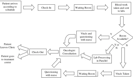
Figure 3.3 illustrates the treatment center process prior to the patient receiving treatment. Patients arrive into the OTC either directly from one of the clinics or in follow-up to prior visits. In either case, upon arrival at the treatment center, patients must first go through a check-in process. A receptionist pulls the patient’s chart and brings it to the charge nurse to notify the charge nurse the patient has arrived. Once the patient checks-in, he or she must wait until several other processes have been completed to ensure the drug is ready to be administered and clearance for treatment has been provided by the oncologist. If the charge nurse deems the health of the patient to be inadequate for the treatment, then the oncologist must be contacted. The charge nurse then receives approval to carry on with the treatment, or instructions on reducing the strength of the regimen. Additionally, if the order has not been entered by the oncologist, the charge nurse must contact the oncologist about the order. Once this process is complete, the pharmacy begins mixing the drug.

Patient arrives according to

schedule Check-In Waiting Roo m

Blood work taken and sent

to labs

Vita ls and questioning

with nurse

Vita ls Taken Lab Processing

in Para llel

Waiting Roo m Questioning with nurse Oncologist Consultation Check-Out Patient Leaves Clin ic

(37)

Figure 3.3: Flow chart of treatment center process prior to treatment being initiated.

Once the order has been verified and the lab results approved, the pharmacy can begin to mix the drug. The pharmacist reviews the order and may contact the physician before mixing the drug. When the pharmacist approves, the order is printed and brought back to pharmacy technicians for mixing. The drug is mixed and then reviewed by a pharmacist in the clean room, the room where the technicians work, before being sent to the treatment center. Next, a treatment center nurse picks up the patient’s chart, locates the patient’s drug, reviews the blood results, and then retrieves the patient from the waiting room for treatment.

Treatment Center Flow Following Pre-Treatment

(38)

reason, we refer to the combination of beds and chairs as chairs throughout the remainder of the thesis. Of the two treatment types, injections and infusions, injections are much shorter. Thus patients receiving injections are typically allocated a chair. Prior to injection the nurse reviews and discusses the appropriate medical history with the patient and provides relevant information about the injection to the patient. Once the injection is complete, the patient is free to leave. There is no discharge process following this step.

Figure 3.4: Flow Chart of treatment center flow process following treatment.

(39)

hours, and 5 hours). Once the infusion is complete, the nurse disconnects the IV and discharges the patient. There is no formal check-out process at the center.

Grouping of Resources in the Treatment Center

In the treatment center, chairs and beds are used on a first-come first-serve basis regardless of patient type. However, the nurses are often organized into pods by disease based groups (DBGs). In general, nurses serve patients from within their own DBG. However, nurses can help out in other DBGs when necessary. There are five major DBG classifications: Breast/Gynecology, Gastrointestinal and Genitourinary (GI/GU), Hematology Oncology (HOA), Lung/thoracic, and off-service. Off-service patients are various disease and regimen types that can be served by any of the nurses (though most typically HOA). All other DBGs have designated nurses to serve those patient types. Patient volume by disease type varies by day of the week, as does total treatment center throughput, and schedules of nurses. Other than nurses, chairs and beds, resources in the treatment center include the charge nurse and the receptionists for check-in.

Sources of Uncertainty

(40)

(41)

Section 2: Methods

We built our simulation model based on the above conceptual model using Rockwell’s simulation software, Arena version 11. We run the model separate for each day of the week because of the significant variation in patient arrival rates in each of the clinics by day of week. Thus, there are five variants of the simulation model in which the input streams are changed based on the day of the week. Preliminary work in developing the model included collecting sample observation times for services provided in all parts of the cancer center. Process maps representing the patient flow process were developed based upon these observations and interviews with subject matter experts. Collaborative work with subject matter experts yielded assumptions for process times where data did not exist or was not immediately available. Additional model data including the number of resources (nurses, doctors, chairs/rooms, receptionists, phlebotomists, etc.) and associated schedules came from a variety of sources, including computer information systems and expert interviews including oncologists, administrators, and nurses for the clinic, treatment center, and pharmacy.

Once data collection was complete, a prototype version of the simulation model was developed. The initial model included major processes within the cancer center including clinics, labs, radiology, pharmacy, and the treatment center. The model was built to include the primary clinics that cancer patients flow through. Some other smaller clinics that send patients to the treatment center were treated as a separate random arrival feeding directly into the treatment center. This arrival stream also includes the small proportion of patients arriving directly into the treatment center. Major components of the simulation model are as follows.

Patient Arrivals

(42)

on the mean number of arrivals through various parts of the day. We used a non-stationary Poisson arrival process because patient arrival rates vary significantly over the course of a day. These arrivals were generated in the model based on historic data from the time period of July 2010 through October 2010. An additional benefit to modeling arrival processes in this manner is the ease in translation for future volume increases, when arrival schedules may not be developed yet.

Our approach is consistent with other studies. For example, Swartzman (1970) performed several statistical tests in a large hospital to determine appropriate ways to model patient arrivals. He concluded that in the case of unscheduled arrivals, a time-varying Poisson arrival rate most closely described arrivals. While our arrivals are not unscheduled, we apply the same principle with our time-varying arrival rate being defined by the number of arrivals over a given period of time based on historical data.

We used the arrival schedule feature in Arena 11 to define the non-stationary Poisson arrival process for each clinic based upon historical arrivals. This feature allows the user to enter in expected arrival rates over user-defined intervals of time. Hourly throughput rates were input for various blocks of time throughout the day. The average expected arrival rate by each half-hour of the day was calculated from the historical data. Arrivals begin at 7:00 am and end at 5:30 pm. The arrival rate for each half-hour was calculated as an equivalent hourly rate for entering the Poisson process into Arena 11.

(43)

Patient arrivals are generated for multiple clinics, which ultimately become arrivals into the OTC. Patient arrivals are also generated for patients directly to the treatment center from other sources. These other sources include the collection of various other clinics not explicitly represented in our simulation model, patients not required to visit an oncologist in the clinic prior to receiving treatment, and patients arriving directly from radiation oncology.

Patient flow process

All components of the patient flow process described in Section 1 of this chapter are included in the simulation model. However, we made some simplifying assumptions in our model. The central labs and radiology are both modeled as general delays with no resources. This means that the length of time a patient spends processing is merely a random sample from the probability distribution of the flow time. We made this assumption for two reasons: 1) the time spent waiting in either of these two areas is accounted for in the historical data used to represent these resources; and 2) the radiology and central labs serve patients from across the entire hospital, and thus, modeling resources and specific process times without the entire patient flow does not make sense.

(44)

Table 3.1: Arrivals per hour calculations for each time block in a clinic on Thursday.

Preparatory work prior to the oncologist visit consists of two pieces: recording vitals, and pre-consult assessment and briefing. Vitals can be performed by either a vitals specialist or a nurse. We assume vitals specialists perform a piece of the preparatory work in cases when the nurse and room are unavailable. This occurs at a small location next to the phlebotomy area. In such cases, the patient returns to the waiting room after having vitals taken, and when the nurse and room become available, the nurse will bring the patient to the exam room and finish preparatory work prior to the consult. Otherwise, the nurse retrieves the patient and completes the full preparatory process in the exam room, provided a room is available.

# Thursdays 18 E[Thursday Arrivals 109.33

E[Arrivals]/half-hour Arrivals/Hour

7-7:30 55 3.06 6.11

7:30-8 111 6.17 12.33

8-8:30 136 7.56 15.11

8:30-9:00 148 8.22 16.44

9:00-9:30 195 10.83 21.67

9:30-10:00 186 10.33 20.67

10:00-10:30 175 9.72 19.44

10:30-11:00 162 9.00 18.00

11:00-11:30 126 7.00 14.00

11:30-12:00 75 4.17 8.33

12:00-12:30 77 4.28 8.56

12:30-1:00 96 5.33 10.67

1:00-1:30 79 4.39 8.78

1:30-2:00 99 5.50 11.00

2:00-2:30 70 3.89 7.78

2:30-3:00 71 3.94 7.89

3:00-3:30 51 2.83 5.67

3:30-4:00 30 1.56 3.11

4:00-4:30 19 0.00 0.00

4:30-5:00 4 0.00 0.00

5:00-5:30 2 0.11 0.22

(45)

We assume patients have an equal probability of seeing any oncologist in the clinic. Each oncologist is assumed to have the same number of exam rooms and mean patient volume. These assumptions were made to simplify construction of the model and due to delays in obtaining the necessary oncologist patient volume information by day of week.

After consultation with a patient, the oncologist enters the chemotherapy order into the computer system for the treatment center and pharmacy. In some cases the order is not entered, subsequently requiring the charge nurse to call the oncologist later in the process to verify the order. To reflect this in the simulation model, each order has a certain probability of requiring nurse follow-up. Probability estimates are based on historical data, and can be found in Table 3.4. Finally, a clinic check-out process is modeled. In some cases, patients do not go through the check out process if they are willing to schedule future appointments by e-mail or phone. We model certain percentages of patients skipping the check-out process based on expert opinion of frequency of occurrence, denoted in Table 3.3 as % late tray patients.

In the treatment center, the time for the charge nurse to evaluate a chart is broken into two parts. The first part is the time it takes the charge nurse to review the order and enter the necessary information. We assume all patients undergo this process initially. The second part is the time required for the charge nurse to review labs and follow-up with the oncologist. This occurs with a certain probability based on the results of a time study. Thus, some patients randomly encounter a second stage to the chart check process for contacting the oncologist. The pharmacy process is also broken down into two parts based upon a time study. The first part is for the pharmacist to check the order and labs and process the paperwork, and the second part is for the technicians to mix the drug. Finally, we assume the scheduled treatment time is a random variable with a discrete 5-point distribution based on current scheduling templates. The value of this distribution can be found in Appendix 3.

Scheduling of Resources

(46)

than specific start and end times for each employee. While the capacity schedule is developed from an actual staff arrival schedule, this subtle difference means staffing levels are modeled from the patient perspective in the sense that the patient is only concerned with how many staff members are available at any given point in time at any given location. Thus, the simulation model has capacity schedules derived from employee schedules. Resources include check-in and check-out receptionists for all clinics, phlebotomists for some of the clinics (some clinics model lab draws as a general delay because patients receive lab draws off clinic-site), nurses and oncologists for each of the clinics (we assume each oncologist has one nurse and three exam rooms after consulting with the administrative manager), exam rooms, receptionists at the treatment center check-in, a charge nurse, nurses by DBGs, treatment chairs, and beds. Many of the resources are available according to predefined schedules. A complete list detailing every employee schedule can be found in the Appendix 4.

Nurses in the treatment center are modeled uniquely to capture their role in both direct and indirect care that results from starting and monitoring patients. We assume that each nurse working has six capacity units available. In the simulation model, this means that for each nurse, there are six units available to be distributed for use by patients. In order for a patient to begin an infusion (direct care time), we require at least 3 units of nurse to be available and unused. Thus, a patient in direct care for start-up uses 3 units of nurse. Once the nurse finishes start-up and moves to a monitoring role with the patient, 2 units of the nurse are freed (1 unit is still in use). Doing so restricts the number of patients a nurse can serve at one time to 4 as desired. For example, if 3 units of nurse are being used, then 3 units are available to start a new patient. Suppose a new patient is now serviced. Once that patient has completed start-up, 4 units of nurse are being used, meaning there are only 2 units of nurse available, an insufficient amount to begin a fifth patient. Thus, we restrict the number of patients to 4 per nurse.

Methodology for Determining Service Time Probability Distributions

(47)

fit using standard statistical data fitting techniques using Arena 11 Input Analyzer, all of which can be found in Appendix 3. Criteria for selecting distributions were visual inspection and the results of chi-square and Kolmogorov-Smirnov tests. Additional consideration was given to the squared error of the fit. For processes with unreliable or no data, probability distributions were fit in two ways; time studies and expert opinion. As time permitted and as it was possible, time studies were performed to collect data for fitting distributions, as described in the paragraph below.

In total, three time studies were performed: one for the pharmacy process in two parts (pharmacist processing time and drug mixing time), one for the check-out time at one of the clinics, and one for the length of the chart check by the charge nurse in the OTC. The pharmacy time study was performed over several days working with both pharmacists and pharmacy technicians during the summer of 2010. A time study for check-out at one of the clinics was performed on September 21, 2010. The time study recorded when the patient walked up to the counter as the beginning of check-out and the time the patient walked away from the counter as the end of check-out. A time study for the charge nurse chart check was performed on October 5, 2010. This time study captures the length of time it takes for a patient chart to be processed, with the start of processing occurring when the charge nurses begins examining the chart, and ending when the charge nurse has placed the chart on the front counter for pickup by the OTC nurse. We broke chart check times into two categories, depending upon the situation. The first category is a normal or routine chart check, meaning the nurse does not have to call externally to complete examination of the chart. The second category is a special case chart check, defined by the charge nurse calling the patient’s oncologist either because the patient’s blood specimen indicated the patient should not receive chemotherapy for health reasons or because the oncologist did not approve the chemotherapy order in the computer system.

(48)

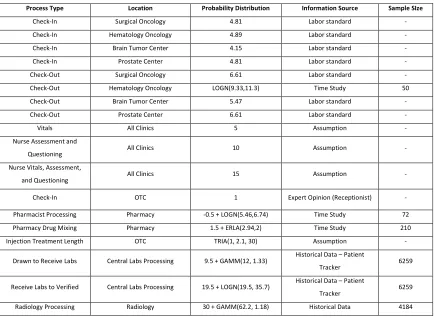
employee time associated with each patient on average. This information comes from both past experiences of the time it takes to process patients, as well as any other incidental non-direct patient contact activities such as filing paperwork or scheduling future appointments online. A labor standard includes a direct patient time component and non-direct patient time component; we use only the direct patient time component in our model. We list the process the probability distribution is for, as well as the source of the information and probability distribution. Historical data sources came from several places, as the hospital we study uses multiple data collection applications. Additionally, we provide a list of information used to split patient routing in the cancer center in Table 3.3.

Table 3.2: List of probability distributions and their sources as used in the simulation model (all times in minutes).

Process Type Location Probability Distribution Information Source Sample SIze

Check-In Surgical Oncology 4.81 Labor standard - Check-In Hematology Oncology 4.89 Labor standard - Check-In Brain Tumor Center 4.15 Labor standard - Check-In Prostate Center 4.81 Labor standard - Check-Out Surgical Oncology 6.61 Labor standard - Check-Out Hematology Oncology LOGN(9.33,11.3) Time Study 50 Check-Out Brain Tumor Center 5.47 Labor standard - Check-Out Prostate Center 6.61 Labor standard - Vitals All Clinics 5 Assumption - Nurse Assessment and

Questioning All Clinics 10 Assumption - Nurse Vitals, Assessment,

and Questioning All Clinics 15 Assumption - Check-In OTC 1 Expert Opinion (Receptionist) - Pharmacist Processing Pharmacy -0.5 + LOGN(5.46,6.74) Time Study 72 Pharmacy Drug Mixing Pharmacy 1.5 + ERLA(2.94,2) Time Study 210 Injection Treatment Length OTC TRIA(1, 2.1, 30) Assumption -

Drawn to Receive Labs Central Labs Processing 9.5 + GAMM(12, 1.33) Historical Data – Patient

Tracker 6259 Receive Labs to Verified Central Labs Processing 19.5 + LOGN(19.5, 35.7) Historical Data – Patient

(49)

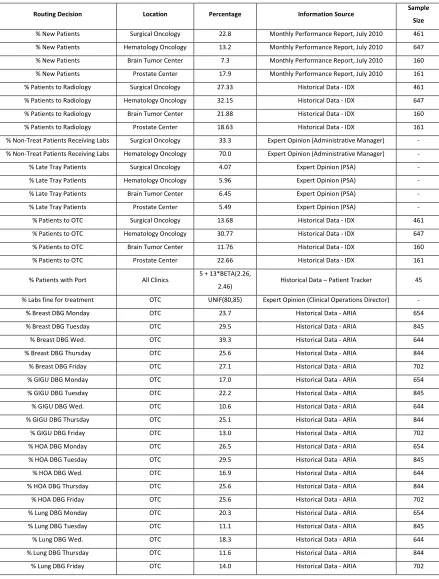
Table 3.3 – List of routing percentages and their sources as used in the simulation model.

Routing Decision Location Percentage Information Source Sample

Size

% New Patients Surgical Oncology 22.8 Monthly Performance Report, July 2010 461 % New Patients Hematology Oncology 13.2 Monthly Performance Report, July 2010 647 % New Patients Brain Tumor Center 7.3 Monthly Performance Report, July 2010 160 % New Patients Prostate Center 17.9 Monthly Performance Report, July 2010 161 % Patients to Radiology Surgical Oncology 27.33 Historical Data - IDX 461 % Patients to Radiology Hematology Oncology 32.15 Historical Data - IDX 647 % Patients to Radiology Brain Tumor Center 21.88 Historical Data - IDX 160 % Patients to Radiology Prostate Center 18.63 Historical Data - IDX 161 % Non-Treat Patients Receiving Labs Surgical Oncology 33.3 Expert Opinion (Administrative Manager) - % Non-Treat Patients Receiving Labs Hematology Oncology 70.0 Expert Opinion (Administrative Manager) - % Late Tray Patients Surgical Oncology 4.07 Expert Opinion (PSA) - % Late Tray Patients Hematology Oncology 5.96 Expert Opinion (PSA) - % Late Tray Patients Brain Tumor Center 6.45 Expert Opinion (PSA) - % Late Tray Patients Prostate Center 5.49 Expert Opinion (PSA) - % Patients to OTC Surgical Oncology 13.68 Historical Data - IDX 461 % Patients to OTC Hematology Oncology 30.77 Historical Data - IDX 647 % Patients to OTC Brain Tumor Center 11.76 Historical Data - IDX 160 % Patients to OTC Prostate Center 22.66 Historical Data - IDX 161 % Patients with Port All Clinics 5 + 13*BETA(2.26,

2.46) Historical Data – Patient Tracker 45 % Labs fine for treatment OTC UNIF(80,85) Expert Opinion (Clinical Operations Director) -

(50)

In the absence of historical data and time studies, initial estimates were made using constant, uniform, and triangular probability distributions based on expert opinion. However, preliminary validation showed that these initial estimations did not appear to correctly represent processes in the cancer center, as many of the processes tend to be centered on a most common time with long narrow tails reflecting process variability. Therefore, it was decided to use Beta distributions for processes with no data. Expert opinion was solicited for the minimum, most frequent (mode), maximum, and average processing times, which were used to define Beta distributions. The following equations were used to calculate the beta distributions using an excel spreadsheet. We used the asymmetry ratio, r, to estimate the shape parameters, α1 and α2. The fit

was determined to be successful if the use of minimum, maximum, and most likely times yielded a probability distribution with a mean that matched the average processing time as provided by the pilot time study or expert estimation. In a very small number of cases, we had a small sample size of time study data available, but with too few data points to find a reasonable fit for a probability distribution. In such cases we also used Beta distribution estimations. In one case, charge nurse chart check time, using the asymmetry ratio approximation yielded a solution with an expected mean that differed from the time study data mean. In this case, with mean and mode values available, a system of equations was solved to determine the beta distribution parameters using the equations for mean and mode listed below. The final distribution fits are shown in Table 3 below.

General Form of Beta Distribution: a= minimum value

b= maximum value m= mode

r= (b-m)/(m-a)

α1= (4 + 3r + r2) / (1+ r2)

α2= (1 + 3r + 4r2) / (1+ r2)

μ = (bα1 + aα2 )/(α1 + α2 )

(51)

Generalized Beta Distribution: a + (b-a)BETA(α1 , α2)

Input Distributions for Service Times

The results of the time studies are as follows. Probability distributions for the pharmacy time study were fit as -0.5 + LOGN(5.46,6.74) for pharmacist processing and 1.5 + ERLA(2.94,2) for drug mixing. For the clinic check out time study, an average time of 8.41 minutes was observed, and the following distribution was fit using Arena’s Input Analyzer: LOGN(9.33,11.3). For the charge nurse chart check time study an average time of 2.5 minutes for regular chart checks and 29 minutes for prolonged chart checks were observed. There was not enough data to get a good probability distribution fit with software, but the average times were useful in combining with expert opinion to develop a distribution. Figure 3.5 below shows an example of a probability distribution fit based upon a time study, for the drug mixing process. All service times were uploaded into Arena’s Input Analyzer, which generated the histogram, goodness of fit, and probability distribution parameters for each potential probability distribution.

(52)

For the distributions that were estimated without data, experts were interviewed. The results of that effort are shown in Table 3.4, with the expert estimates of minimum, most likely (mode), and maximum time provided, along with the average if a pilot time study was performed. The probability distribution fit is provided in the final column. Beta distributions were used because the nature of the process is that the bulk of the probability mass is concentrated at some lower value near the mode with a long tail representing potential complications associated with certain complex patients. In the case of percent of unfilled orders, a triangular distribution was actually believed to be more consistent with the mean from the pilot time study. Additionally, in cases where we received multiple responses in an expert opinion survey, we averaged the values of each parameter to achieve our input parameters for the model. Asterisks are used in the table to denote process types were not calculated using the asymmetry ratio, but rather by solving a system of equations based on the input of average and mode obtained from time study data.

Table 3.4: Processes analyzed for fitting without data; parameter estimates and distribution fit based on expert opinion (minutes where applicable for time units).

Process Type Min. Mode Max. Average Distribution Fit

Blood Draw, Port 15 20 30 20 15 + 15*BETA(2.80, 4.60) Blood Draw, No Port 3 9 19 10 3 + 16*BETA(3.12, 4.53) Doc Consult Length New Patient 20 45 75 45 20 + 55*BETA(3.70, 4.25) Doc Consult Length Return Patient 10 17.5 45 20 10 + 35*BETA(1.97, 4.55)

Time for Doc to Enter Order into

Computer 1 2 5 2 1 + 4*BETA(2.20, 4.60) Charge Nurse Chart Check* 0.5 1 38 2.5 0.5 + 37.5*BETA(1.30, 23.06)

% of Unfilled Orders 82 85 86 - TRIA(82, 85, 86) Time for Unfilled Orders to be Called

In* 4 16 100 29 4 + 96*BETA(1.48,4.36) OTC Nurse Chart Check 2 5 17.5 - 2 + 15.5*BETA(1.84, 4.52) OTC Nurse Set-up Time for

Treatments 5 15 30 - 5 + 25*BETA(3.31, 4.46) HR 1 Infusion Type Treatment

Length 15 60 90 - 15 + 75*BETA(4.46, 3.31) HR 3 Infusion Type Treatment

Length 90 80 210 - 90 + 120*BETA(4.60, 2.20) HR 5 Infusion Type Treatment

Length 210 330 480 - 210 + 210*BETA(4.36, 3.52)

* corresponds to a process where probability distribution was fit by taking the average and mode values to solve a system of equations for parameters α1 and