Emissivity Estimation of Cryogenically Cooled Materials Using a Numerical Technique

(1)

ISSN(Online): 2319-8753 ISSN (Print) : 2347-6710

I

nternational

J

ournal of

I

nnovative

R

esearch in

S

cience,

E

ngineering and

T

echnology

(A High Impact Factor, Monthly, Peer Reviewed Journal)

Visit: www.ijirset.com

Vol. 6, Issue 11, November 2017

Emissivity Estimation of Cryogenically Cooled

Materials Using a Numerical Technique

Jithin P Raj 1, Manu M John 2

P.G. Student, Department of Mechanical Engineering, College of Engineering, Adoor, Kerala, India1

Associate Professor, Department of Mechanical Engineering, College of Engineering, Adoor, Kerala, India 2

ABSTRACT: Thermal shields cooled from 120K down to 80K are used to enclosing accelerator cryomodules for reducing thermal load. A precise knowledge about the low temperature emissivity of materials having a decisive importance in designing passively cooled components operating at low temperature. This paper describes a numerical technique for measuring the emissivity of materials in the temperature range of 80K to 120K. In this paper emissivity estimation of copper and aluminium samples are presented at different temperature and different geometric parameter combinations and the results are confronted with other experimental results. COMSOL Multiphysics software is used for analysis.

KEYWORDS:Cryomodule, Emissivity, Thermal shield.

I. INTRODUCTION

Thermal radiation even at low temperature is important when conduction and convection heat transfer are minimized, as under certain vacuum situations found in space simulators and cryogenic storage vessels [1]. The study of material emissivity in the low temperature range is of interest in many fields, such as the one concerned with space application [2] and solar energy utilization [3].

High-gradient high-duty cycle accelerators use superconducting niobium RF cavities operating at 1.8 – 4.5K. To minimize the heat leak to these low temperature the 1.8 – 4.5K accelerator components, the cold mass, are enclosed by thermal shields cooled to 80 – 120K [4]. For connecting the support structure and RF power couplers, holes are provided on the thermal shield which face room temperature. Thermal baffles are installed in those holes to reduce the open area and the radiative heat leak. The surfaces of thermal baffles from which the reflection occurs should have a high absorption, i.e., a high emissivity. So that, those surfaces are coated with black paint.

Radiometric technique and the Calorimetric technique are the two different techniques used in this cryogenic temperature range. In the radiometric technique, the radiation flux emitted from the sample is measured directly and is compared with black body radiation at the same temperature by means of very sensitive bolometers; this method permits both directional and spectral emissivity measurements [5]. In the calorimetric technique, the total hemispherical emissivity of surface is measured by studying the cooling process of an insulated specimen [6].

On space missions passive cooling is used to keep low temperature of components. The radiating surfaces of thermal control systems are provided with high-emissivity coatings. Stefan-Boltzmann Equation describes the radiation of heat from a surface.

(1)

Where Q˙ is the total radiated power in Watts, T is the surface temperature in Kelvin, A is the surface area in m2_{, ε is}

(2)

I

nternational

J

ournal of

I

nnovative

R

esearch in

S

cience,

E

ngineering and

T

echnology

The objectives of the present study is to determine the emissivity of copper and aluminium sample cooled from 120K to 80K, the effect of vertical position of sample on resultant emissivity, and to compare the estimated value with other existing experimental results.

Paper is organized as follows. Section II describes geometrical information, which includes layout of geometry with thermal loads and the dimension of geometry. View factor is calculated for different geometrical parameter combinations. Numerical analysis is given in Section III. Section IV presents experimental results that plotted on graphs for comparison. Finally, Section V presents Summary and conclusion.

II. GEOMETRICALINFORMATION

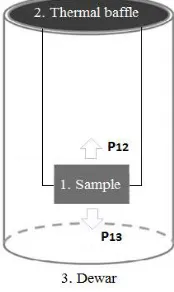
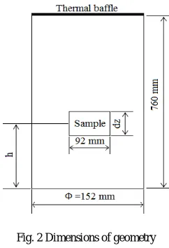
Schematic drawing of the geometry with thermal load and layout are shown in Fig.1. Fig.2 shows the dimensions. The sample is in the form of a thin rectangular foil. The thickness of sample is 1mm, width is 92mm. The height of sample is denoted as (dz) and the vertical position of sample centre is denoted as (h). The sample is suspended inside a stainless steel dewar whose walls are maintained at a constant temperature 120K. The thermal baffle act as the top wall of cylindrical dewar. Inner face of thermal baffle is coated with black paint whose emissivity value is 1 and is maintained at a constant temperature 150K.

Fig. 1 Layout of geometry with thermal load

A pressure of 10-7 torr was maintained inside the vacuum chamber since residual gas conduction was negligible. The

radiated power from sample surface to thermal baffle (P12) and radiated power from sample surface to inner surface of

cylindrical dewar (P13) are two important thermal loads that affecting the sample temperature. The change of (P12) is

very small on compared to (P13) and is neglected at equilibrium temperature.

At equilibrium temperature the only one thermal load that affects the sample temperature is (P13)

P13 is defined by [8]

P13 =

(3)

I

nternational

J

ournal of

I

nnovative

R

esearch in

S

cience,

E

ngineering and

T

echnology

Where is Stephan - Boltzmann Constant, T1is sample temperature, T3 is dewar temperature, A1 is the sample surface

area, A3is the dewar surface area, ε1 andε2are the emissivity of sample and dewar respectively and F13 is the view

factor.

Fig. 2 Dimensions of geometry

The view factor in Eq.3 is a function of the system geometry and is defined as [8]

(3)

The sample temperature T1 is changed from 80K to 120K but the dewar temperature and thermal baffle temperature are

made constant at 120K and 150K respectively. Geometrical parameters are shown in Fig.2. The view factor is evaluated numerically using COMSOL Multiphysics. The view factor is calculated at different sample height and vertical position and are summarized in Table1. The thermal baffle surface area and cylindrical dewar surface area are

completely enclosed the sample surface area so the summation of view factor F12 and F13 become one. Since the thermal

baffle has a simpler geometry than cylindrical dewar, so it is easy to calculate the surface area of thermal baffle for

view factor calculation. F12 is calculated first and F13 is then derived. The dewar inner surface material is stainless steel

and ε3 is assumed to be 0.12 ~ 0.25 [9].

Table 1. Variation of view factor when the geometrical parameters changes

Geometrical parameters View factors

Sample height dz(mm) Sample vertical position h(mm) F12 F13

51 455 0.004 0.996

51 125 0.0006 0.9994

(4)

I

nternational

J

ournal of

I

nnovative

R

esearch in

S

cience,

E

ngineering and

T

echnology

III. NUMERICALANALYSIS

Two - dimensional heat conduction equation in steady state is used to evaluate the temperature of metal samples with reasonable accuracy

(4)

Where is sample thickness, and are the temperature averaged thermal conductivity and surface emissivity,

respectively [10]. The factor 2 in the radiation term of Eq.4, accounts for both sides of the sample. Simple finite difference method is used to solve the Eq.4 numerically. The grid were fine enough to give results. The elements are

rectangular in shape with Δx as the length of element along horizontal direction and Δy as the same along vertical

direction. The conduction term in Eq.4 are approximated for a node of mesh at x=m.Δx and y=n.Δy

The linearized expression of radiation term is defined as

(5)

(6)

Where TM is mean temperature and is defined as

(7)

Dirchlet boundary condition are applied. In order to treat the constant term in Eq.7 and averaged thermal conductivity, the numerical process starts with initial guess and the improved value is given for repeated calculation until the criterion of convergence satisfied.

IV. RESULTS ANDDISCUSSION

Emissivity results at temperature between 80K and 120K are estimated for copper and aluminium samples. The emissivity values of copper and aluminium sample are plotted to corresponding temperature are shown in Fig.3 (a) and (b) respectively.

(5)

I

nternational

J

ournal of

I

nnovative

R

esearch in

S

cience,

E

ngineering and

T

echnology

Fig. 3 Emissivity vs Temperature of samples, (a) Copper sample, (b) Aluminium sample

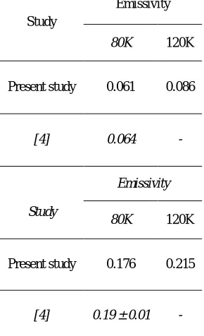
Table 2. Estimated surface emissivity compared with listed values in reference, (a) Copper sample, (b) Aluminium sample

Study

Emissivity

80K 120K

Present study 0.061 0.086

[4] 0.064

-Study

Emissivity

80K 120K

Present study 0.176 0.215

(6)

I

nternational

J

ournal of

I

nnovative

R

esearch in

S

cience,

E

ngineering and

T

echnology

Table 3. Estimated surface emissivity for different vertical position of sample at 80K

Sample

Emissivity

dz1 dz2

Copper 0.061 .0615

Aluminium 0.176 0.177

The emissivity estimated for copper is 0.061 at 80K and the literature value is 0.064 at 80K [4]. The estimated emissivity value is 4.68% smaller than literature value. A possible reason for this difference is due to the increase in reflection from the surface and associated secondary radiation. Table 2 compares the estimated emissivity with reference values. Similar inspection and discussion are made for the aluminium sample. The emissivity is in the range of 0.176 - 0.215, which is 7.36% smaller than experimental value at 80K.

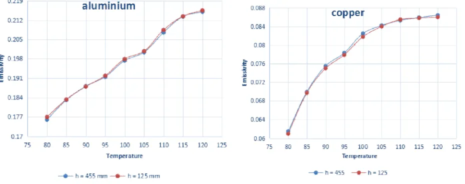
The column titled dz1in table 3shows the range of emissivity estimated for sample which was suspended 125 mm from

bottom of the dewar, similarly column titled dz2 shows the range of emissivity estimated for sample which was

suspended 455 mm from bottom of the dewar.

Fig. 4 Emissivity vs Temperature of copper sample at different vertical positions, (a) Copper sample, (b) Aluminium sample

(7)

I

nternational

J

ournal of

I

nnovative

R

esearch in

S

cience,

E

ngineering and

T

echnology

Table 4. Estimated surface emissivity of sample with different surface area at 80K

Sample

Emissivity

dz1 dz2

Copper 0.061 0.0618

Aluminium 0.176 0.1766

Table 4 shows the estimated surface emissivity of samples at different surface areas. The height of sample dz1 is 51mm and dz2 is 102. Result shows that only less than 1% difference in emissivity was appeared while changing the sample surface area. The change in surface area has negligible impact on surface emissivity.

V. SUMMARYANDCONCLUSION

The emissivity value of copper and aluminium sample from 120K down to 80K are estimated numerically. The result presented here show good agreement between the estimated value and literature value. This suggest that the method is correct. Surface emissivity of copper sample is estimated to be 0.061 at 80K, which is lower than literature value. Secondary radiation is the major cause for this difference. The aluminium surface at 80K has a high emissivity of 0.176, which is well confronted within the range of literature value. Change in geometrical parameters does not have significant effect on surface emissivity. The estimated emissivity values of copper and aluminium from 80K - 120K helps to select those materials for proper application in future cryomodules in the same temperature range.

REFERENCES

[1] K.H Hawks, W.B Cottinghaam 1971 Total normal emittances of some real surfaces at cryogenic temperatures Advances in Cryogenic Engineering

[2] S.S Penner, L Iceman 1975 Energy Vol. 21 (London: Addison-Welsey) pp 347-52) [3] J.C Richmond 1963 Measurement of Thermal Radiation Properties of Solids: NASA SP-31

[4] S.H Kim, Z.A Conway P.N Ostroumov, and K.W Shepard 2014 Emissivity measurement of coated copper and aluminum samples at 80K AIP Conference Proceedings 1573,

[5] K. H Hawks 1969 PhD Thesis Purduce University [6] J.R Jack, E.W Spisz 1970 NASA TND - 5651

[7] J.Tuttle, E.Canvan, M.Dipirrol, X.Lil J. Tuttle1, E. Canavan1, M. DiPirro1, X. Li1, R. Franck, and D. Green 2012 A High-Resolution Measurement of the Low-Temperature Emissivity of Ball Infrared Black Advances in Cryogenic Engineering AIP Conference Proceedings 1434, 1505-1512

[8] A. J. Chapman, Heat Transfer, New York: The Macmillan Company, 1967, pp. 430-457.

[9] W. Obert, J. R. Copland, D. P. Hammond, T. Cook, K. Harwood, Emissivity Measurement of Metallic Surfaces used in Cryogenic Applications Advances in Cryogenic Engineering, Vol. 27