The Genealogy of Sequences Containing Multiple Sites Subject to Strong Selection in a Subdivided Population



The Genealogy of Sequences Containing Multiple Sites Subject to Strong

Selection in a Subdivided Population

Magnus Nordborg

1

_{and Hideki Innan}

2

Molecular and Computational Biology, University of Southern California, Los Angeles, California 90089-1340

Manuscript received August 7, 2002 Accepted for publication December 17, 2002

ABSTRACT

A stochastic model for the genealogy of a sample of recombining sequences containing one or more sites subject to selection in a subdivided population is described. Selection is incorporated by dividing the population into allelic classes and then conditioning on the past sizes of these classes. The past allele frequencies at the selected sites are thus treated as parameters rather than as random variables. The purpose of the model is not to investigate the dynamics of selection, but to investigate effects of linkage to the selected sites on the genealogy of the surrounding chromosomal region. This approach is useful for modeling strong selection, when it is natural to parameterize the past allele frequencies at the selected sites. Several models of strong balancing selection are used as examples, and the effects on the pattern of neutral polymorphism in the chromosomal region are discussed. We focus in particular on the statistical power to detect balancing selection when it is present.

C

OALESCENTtheory is based on the realization that require infinitely many virtual branches; from a practical

selective neutrality allows the separation of descent point of view, simulation of strong selection becomes from state. This makes it possible to model samples (or extremely inefficient because of the large number of populations) as random genealogies with superimposed virtual branches.

neutral mutations (seeNordborg2001). Neutrality is The second way, first described in the context of the thus fundamental to this approach. Nonetheless, selec- coalescent byKaplanet al.(1988), utilizes the fact that tion has been successfully incorporated in two very dif- a polymorphic population can be thought of as

subdi-ferent ways. vided into allelic classes, within which no selection

oc-One way is to construct a genealogical process that curs. Genealogies can then be modeled using existing “leaves room” for selection by creating genealogies that models of geographic subdivision, with mutation (and, contain “virtual” branches representing possible lines in a sense, recombination) taking the place of migra-of descent. After mutations have been superimposed tion. It is necessary to know the past (relative) sizes of and the state transmitted through each branch is known, the “subpopulations,”i.e., of the allelic classes. Thus the the genealogy is “pruned” by preferentially removing approach may be seen as modeling genealogies condi-selectively inferior branches so that only “actual” lines of _tionalon the past frequencies of the selectively different descent remain. The process known as “ancestral selection _{alleles (Nordborg 1999, 2001). However, since it is} graph” (Kroneand Neuhauser 1997;Neuhauser and _{in general not known how to obtain theunconditional}

Krone1997) accomplishes this (see alsoDonnellyand _{process when the past allele frequencies are random}

Kurtz 1999; Neuhauser 1999; Slade 2000a,b, 2001; _{variables, the approach has been used only for strong}

Fearnhead 2001). An important feature of this ap- _{selection, when it may be reasonable to model the}

selec-proach, which can be seen as a natural extension of the _{tive dynamics deterministically. Examples include} bal-standard neutral coalescent, is that all selection coeffi- _{ancing selection (seeHudsonandKaplan1988;} Taka-cients must be scaled using the standard coalescent/ _{hata 1990;Hey1991; Kaplanet al. 1991;Nordborg} diffusion scaling. This means that it is not possible to _{1997, 1999; Takahata and Satta 1998; Kelly and} model arbitrarily strong selection this way: From a math- _{Wade2000;Schierupet al.2001;BartonandNavarro} ematical point of view, infinitely strong selection would _{2002; Navarro and Barton 2002), positive selection} (or “selective sweeps,” seeKaplanet al.1989;Hudson

et al.1994;Bravermanet al.1995;Simonsenet al.1995;

KimandStephan2002;Przeworski2002), and

purify-1_{Corresponding author:Molecular and Computational Biology,}

Uni-versity of Southern California, SHS 172, 835 W. 37th St., Los Angeles, _{ing selection (or “background selection,” seeHudson} CA 90089-1340. E-mail: [email protected]

andKaplan 1995;Nordborg1997;Campbell1999).

2_{Present address:Human Genetics Center, School of Public Health,}

The two approaches are in a sense complementary: University of Texas Health Science Center, 1200 Hermann Pressler,

Houston, TX 77030. Whereas the ancestral selection graph works only for

weak selection, the conditional approach works only for

yi,k(t)⫽

1 2

冢

兺

i

j⫽1

xji,k(t)⫹

兺

H

j⫽1 xij,k(t)

冣

.

strong selection. How to connect the two is not clear. In this article we use the second, conditional approach,

Lety⬘i,k(t) be the frequency of haplotypeiamong the

ga-to show how the original formulations of Kaplan et

metes produced in patch k, generation t. In general, al. (1988) and Hudson and Kaplan (1988) may be

these gamete frequencies will be functions of the adult extended to model selection at multiple sites, with the

genotype frequencies and the appropriate segregation, possibility of different selection coefficients in different

mutation, and recombination parameters. Let subpopulations (local adaptation). This has been done

before (Takahata1990;Kaplanet al.1991;Nordborg

y″i,k(t)⫽

兺

P

l⫽1y⬘i,l(t)clflk

fk(t)

1997, 2001;KellyandWade2000;Schierupet al.2000;

BartonandNavarro2002); however, most treatments

be the frequency of haplotypeiamong the male gametes have considered the genealogy of a nonrecombining

in patch kafter migration (female frequencies are of site linked to the selected loci. In contrast, we consider

course unaffected by migration), where the genealogy of the entire region. This makes it

possi-ble to ask statistical questions about the pattern of

poly-fk(t)⫽

兺

H

j⫽1

兺

P

l⫽1

y⬘j,l(t)clflk.

morphism (see alsoInnanandTajima1999;Schierup

et al.2001;KimandStephan2002;Przeworski2002).

Zygotes are then formed by random union of gametes In particular we are interested in the conditions under

within patches, so the frequency of genotype {i,j} among which we would expect to be able to detect balancing

the zygotes in patchkis selection.

x″ij,k(t)⫽

冦

y⬘i,k(t)yi″,k(t), i⫽j,

y⬘i,k(t)y″j,k(t)⫹yj⬘,k(t)y″i,k(t), i⬆j.

A BASIC MODEL

Consider a diploid, hermaphroditic population con- Let the relative viability of a zygote with genotype {i,j} sisting ofPpatches, each of which harbors a constant, in patchkbe 1⫺ wij,k(t), and define

large number of adult individuals,Nk,k⫽ 1, 2, . . . ,P.

Let N ⫽ 兺Nk be the total population size, and define x⵮ij,k(t)⫽

x″ij,k(t)[1⫺wij,k(t)]

wk(t)

, ck⫽Nk/N. The population reproduces in discrete,

non-overlapping generations according to a generalized _where Wright-Fisher model in the following manner. Each

in-wk(t)⫽ 1⫺

兺

iⱕj

x″ij,k(t)wij,k(t).

dividual produces an (effectively) infinite number of gametes. Male gametes (e.g., pollen) flows between the

The next generation of adults in patch k is formed by patches; let fkl be the probability that a male gamete

drawingNkindividuals according to these “postselection”

produced in patchkends up in patchl. After migration,

frequencies. Thus, conditional on the genotype frequen-gametes unite randomly to form zygotes. The number

cies among adults in generationt, the length-Gvector of immature individuals in each patch is thus still

effec-tively infinite, but only a finite number (Nkin thekth [_N11,k(_t⫹1) _N12,k(_t⫹1) . . . _NHH,k(_t⫹1)]

patch) reach adulthood. The probability that a given

is multinomially distributed with parametersNkand

individual survives is determined by its genotype and

the genotypic frequencies in the patch. Generalizations _[x⵮11,

k(t) x⵮12,k(t) . . . x⵮HH,k(t)].

of this model are discussed below.

Genealogy of the surrounding segment: Consider a

Forward dynamics at the selected loci: Let Hbe the

chromosomal segment that contains the selected locus or number of different haplotypes with respect to the selected

loci. Take a particular copy of this segment, sampled from locus or loci (which are assumed to be linked). Label the

the adult individuals in generationt⫹1. With respect to haplotypes 1, 2, . . . ,H, and theG⫽H(H⫹1)/2 different

geographic location, it belongs to one of thePpatches, genotypes by pairs of indices {i,j},iⱕj⫽1, 2, . . . ,H,

and with respect to the selected locus or loci, it belongs according to their haplotypic composition. LetNij,k(t) be

to one of theHhaplotypes. the number of adults with genotype {i, j} in patchk in

Trace the genealogy of this segment one generation generationt. Note that whereasNij,k(t) is a random

vari-back in time. Each nucleotide in the segment in the able,Nkis not. The frequency of genotype {i,j} in patch

current generation is a copy of the homologous nucleo-kis

tide in some parental segment in the previous genera-tion. In the absence of recombination, all nucleotides xij,k(t)⫽

Nij,k(t)

Nk

, _{must have the same parental segment; otherwise, they}

Figure 1.—Two exam-ples of the effects of recom-bination on the single-gen-eration genealogy of a seg-ment. The colors denote an-cestry (only). On the left, a segment with a single-locus

A1haplotype was produced through recombination in anA1/A2heterozygous indi-vidual. As a result, going back in time, one piece of the segment takes on theA2haplotype, whereas the other (containing the locus defining the haplotype) remains A1. On the right, a segment with a two-locusA1B2 haplotype was produced through recombination in anA1B1/A2B2doubly heterozygous individual, causing both pieces to change haplotype (going back in time).

abstractly as a continuous unit interval where each point probabilities through meiosis can readily be derived, but the expressions depend on the details of the model may have a different genealogy. This makes

mathemati-cal and computational sense and does not entail any (e.g., on the number of loci). In general, the probability that a gamete of typeiin patchkresulted from a particu-loss of biological generality (see,e.g.,Nordborg2001).

When tracing the genealogy of the segment back lar type of meiotic event in a particular genotype is a function of the length-G vector [xij,k(t)]iⱕj and the

re-through the life cycle, the first thing to note is that

selection cannot affect its state with respect to either combination and mutation parameters.

Once the genotype and patch of the parental individ-patch or haplotype. The chosen segment must have

been present in one of the gametes of the same type ual has been determined, all eligible individuals are equally likely to have been the parent. Segments can in the same patch before zygotes were formed and

selec-tion took place. However, migraselec-tion can change the thus be seen as “picking” their parent randomly. To trace the single-generation genealogy ofncopies state of the segment with respect to patch, because the

gamete may have been an immigrant, if it was male. of the segment, note that, since infinitely many gametes are produced, and gametes unite randomly within The probability that a randomly chosen gamete of type

iin patchkwas male isy″i,k(t)/[y″i,k(t)⫹ y⬘i,k(t)], and the patches, the fate of each segment is independent of the

fates of all the other segments. In other words, each probability that a male gamete of type i currently in

patchkwas produced in patchlis segment “picks” its parental segment (or segments, in

case of recombination) independently of the other seg-ments. Whenever two or more segments pick parental y⬘i,l(t)clflk

fk(t)y″i,k(t)

⫽ y⬘i,l(t)clflk

兺

P

m⫽1y⬘i,m(t)cmfmk

. (1)

segments belonging to the same patch, haplotype, and genotype, two or more of them may pick the same one. Note that migration always changes the state of theentire

Segments that pick the same parental segment are said segment, because a gamete either does or does not

tocoalesce; if their genealogy is to be traced farther back migrate.

in time, only the single segment needs to be followed. Having traced the segment through migration to the

Segments can of course pick only the same parental premigration gamete pool, the next step is to trace it

segment if they first pick the same parental individual. through gamete production to the previous adult

genera-Since all individuals of the same genotype are equally tion. Gamete production,i.e., meiosis, can change the state

likely to be picked, the probability thatn segments all of the segment with respect to haplotype both through

pick different parents, given that they all pick parents mutation at one of the selected loci and through

recom-with genotype {i,j} in patchkis bination inside the segment. If the gamete was a mutant,

then the segment changes state to take on the haplotype

N⫺n ij,k(t)

兿

n⫺1

m⫽0

(Nij,k(t)⫺m)⫽

兿

n⫺1

m⫽1

冢

1⫺ m

Nij,k(t)冣

. (2)

of the parental segment. If the gamete was a recombi-nant, things are more complicated, because the segment

When two segments pick the same parental haplotype then has two parental segments. At each breakpoint,

in the same parental individual, they coalesce with prob-the parentage of prob-the offspring segment switches from

ability one-half if that individual is homozygous (so that one parental segment to the other. Going backward in

there are two possible parental segments) and with prob-time, the segment splits into two pieces (or sets of pieces

ability one if it is heterozygous (so that only one segment if there was more than one breakpoint), one of which

is possible as parent). takes on the haplotype of the first parental segment

while the other takes on the haplotype of the second parental segment (see Figure 1). Both parental

seg-COALESCENT APPROXIMATION ments consequently have to be followed if the genealogy

of the original segment is to be traced farther back in The purpose of the preceding section was to demon-strate that, conditional on the P length-G vectors [Nij,k

(t)]iⱕj,k⫽1, 2, . . . ,P, fort⫽0,⫺1, . . . ,i.e., conditional good approximation in what follows. Note that Equation

3 implies x⵮ij,k⫽xij,k⫽xˆij,k, and similarly for the

haplo-on the genotype frequencies in all past generatihaplo-ons, it

is possible to model the genealogy ofnsegments sam- type frequencies.

Scaling:Under the assumption that the genotype

fre-pled in generationt⫽0 as a discrete-time Markov

pro-cess running backward in time. However, the interesting quencies can be treated deterministically, it is possible to use standard arguments to find a continuous-time process is the unconditional one, in which the genotype

frequencies are governed by another discrete-time Mar- coalescent approximation for the discrete-time genea-logical process described above. Note that the probabil-kov process, running forward in time (as described

above). Typically, we would like to know how the geneal- ity (2) can be rewritten ogy is affected by theparametersof that forward process

(e.g., the selection coefficients and population sizes),

兿

n⫺1

m⫽1

冢

1⫺ m

Nckxˆij,k

冣

⫽ 1⫺

冢

n 2

冣

Nckxˆij,k

⫹ O

冢

1

N2

冣

. (4) nothow it is affected by a particular realization of it.

Clearly, the unconditional process could be studied

through discrete-time simulation: One would simply Thus, a coalescence event occurs with probabilityO(1/N) simulate the genotype frequencies forward in time and per discrete generation, and it is natural to turn the process then simulate the genealogy backward in time, condi- into a continuous-time process by rescaling time in units

tional on those frequencies. of O(N) generations and letting N go to infinity (while

An alternative approach, which is taken here, is to keepingckconstant to ensure that all the patches become

use a coalescent/diffusion approximation and assume large). The standard scaling of 2Nis used throughout. that the genotype frequencies can be treated as having The per-generation probabilities of migration, muta-evolved deterministically on the continuous timescale tion, and recombination are also assumed to beO(1/N),

(Kaplanet al.1988). It follows from the standard diffu- and the corresponding scaled parameters are

intro-sion arguments of population genetics (see,e.g.,Neu- duced. Thus, it is assumed that the migration probability

hauser 2001) that this may be justified if selection is fklcan be written

sufficiently strong relative to the inverse of the

popula-tion size (or, in the present case, patch sizes). It should fkl⫽

φkl

4N⫹ O

冢

1

N2

冣

, k⬆l, be stated clearly that this approach is not mathematically

rigorous, but it is likely that it can be made rigorous for

whereφklis the migrationrate(recombination and

muta-some scenarios and that it will be a reasonable

approxi-tion are introduced below). Similarly, it is assumed that mation for many others.

all the selection coefficients areO(1/N) (but still large We focus on strong balancing selection in the

follow-enough for Equation 3 to hold approximately; see ing because the approach is easiest to explain and justify

above). Taken together, these assumptions ensure that, for such models (with balancing selection, the model

toO(1/N), is very close to that of Barton and Navarro 2002).

Balancing selection is here simply meant as any form _x″

ij,k⬇ x⬘ij,k⬇xˆij,k,

of selection that tends to maintain all genotypes at

con-and that, to the same order of approximation, stant, nonzero frequencies, which we denotexˆij,k. In a

finite population, the actual frequencies in any given

xˆij,k⬇

冦

yˆ2

i,k, i⫽j,

2yˆi,kyˆj,k, i⬆j. (5)

generation will of course differ from these values. Simi-larly, in the diffusion approximation, the actual

frequen-cies at a given point in time will differ from their expecta- To proceed farther we must consider specific genetic tions. The differences will tend to be smaller the models.

stronger the selection. Note that nothing in the basic Single-locus example:Consider a segment that con-model described above limits how strong selection may tains a locus (or site) that is maintained polymorphic for be. Indeed, it is possible to assume infinitely strong two alleles by strong balancing selection in a subdivided selection (i.e., the selection coefficients need not be environment. There areH⫽2 “haplotypes,”A1andA2, scaled in the diffusion approximation), in which case and three genotypes,A1A1,A1A2, andA2A2. Letaijbe the

probability that alleleAi mutates toAj during meiosis,

xij,k(t)⫽xˆij,k, ∀i,j,k,t, (3)

and letr be the probability of a recombination event. and treating the genotype frequencies as constant is It is assumed that these can be written

evidently justified. However, as discussed inNordborg

(1999), infinitely strong selection significantly compli- _{aij⫽ ␣}ij

4N ⫹O

冢

1

N2

冣

, i⬆j, cates the algebra (because it causes deviations from

Hardy-Weinberg equilibrium) without significantly af- _and fecting the results, and we therefore do not assume that

selection is infinitely strong, but that it is nonetheless _{r⫽ ␳}

where ␣ij and ␳ are the mutation and recombination it can be shown that the probability thata pair out of

nsegments of typeiin patchkcoalesces is rates. This model is identical to previously published

models (HudsonandKaplan1988;Kaplanet al.1988,

1991;Hey1991;Nordborg1997), except that it consid-

冢

n 2

冣

2Nckyˆi,k

⫹ O

冢

1 N2

冣

. ers the genealogy of a segment rather than of a point.

Consider the backward transitions for a single

seg-ment with haplotypei sampled from an individual in Given these transition probabilities, the limiting coa-patchk, as before. Because the probabilities of migra- lescent process can be derived using standard argu-tion, mutaargu-tion, and recombination are all assumed to ments. Segments belong to states with respect to haplo-be small, it is clear that the segment is most likely to haplo-be type and patch as before. Measure time in units of 2N a copy of a segment with the same haplotype in the generations, and let N go to infinity. Then, indepen-same patch in the previous generation. Indeed, it is easy dently of all other segments, each segment with haplo-to show that the probability is 1 ⫺ O(1/N). Further- typeiin patchkmigrates to patchlat rate

more, given that its state with respect to haplotype and

patch did not change, the probability that it was pro- clyˆi,l

2ckyˆi,k

φlk/2 ,

duced by an {i,j} individual isyˆj,k⫹O(1/N). It can also

be shown that the segment is an immigrant of the same _{mutates to haplotypej⬆iat rate} type from patchlwith probability

yˆj,k

yˆi,k

␣ji/2 ,

1 2·

clyˆi,l

ckyˆi,k

flk⫹O

冢

1 N2

冣

,

and recombines with a j haplotype at rate yˆj,k␳/2. If

there are currentlynsegments with haplotypeiin patch a mutant haplotype j ⬆ i from the same patch with

k, the total rate of migration tolis thus probability

n clyˆi,l 2ckyˆi,k

φlk/2 ,

yˆj,k

yˆi,k

aji⫹O

冢

1 N2

冣

,

etc. Similarly, each pair of segments with haplotypeiin and a recombinant from an {i,j} individual in the same

patchkindependently coalesces at rate 1/(ckyˆi,k), so that

patch with probability

the total rate fornsuch segments is

yˆj,kr⫹O

冢

1

N2

冣

.

冢

n 2

冣

ckyˆi,k

. All other transitions (e.g., the segment is an immigrant

mutant) have probabilityO(1/N2_{) or less.}

Two-locus example:Consider a model with two loci

As discussed above, it is simple to extend to a sample _{each with two alleles,A1/A2andB1/B2. There areH⫽} ofnsegments, because the single-generation transitions _{4 haplotypes:A1B1,A1B2,A2B1, andA2B2, which are} num-are mutually independent. Only the coalescence proba- bered 1, . . . , 4 in the order listed, and 10 genotypes. bilities need to be determined. From Equation 4 a single Define the mutation probability at theB-locus,bij,

analo-coalescence event has probabilityO(1/N) or less, which gously toaij. The recombination probability, r, is also

means that the probability of more than two segments defined as before, but letdrbe the length of the part coalescing in a single generation has probabilityO(1/N2_{) that lies between the two loci (which are loci in the} or less. It also means that the probability that a segment strict sense of the word—i.e., there is no recombination involved in a coalescence is a migrant, mutant, or recom- within them; they can be thought of as single-nucleotide binant isO(1/N2_{). The only coalescence event that has polymorphisms, for example).}

probabilityO(1/N) is thus between two segments that The single-generation backward transition probabili-do not change state with respect to haplotype or patch. ties can be found in the same manner as in the single-For simplicity, consider the probability that n ⫽ two locus model, but are in some cases more complicated. segments with haplotypei in patch kcoalesce. To do The probability that a segment of type i in patch kis so, they must have been produced by individuals of the an immigrant of the same type from patchlis

same genotype, by the same individual of that genotype,

and by the same segment within that individual. The 1

2· clyˆi,l

ckyˆi,k

flk⫹O

冢

1

N2

冣

, (6)

probability of this is

as before. The mutation probabilities depend on the yˆ2

i,k·

1

Nckxˆii,k

·1 2⫹yˆ

2 j,k·

1

Nckxˆij,k

· 1⫹O

冢

1 N2

冣

⫽

1 2Nckyˆi,k

⫹O

冢

1

N2

冣

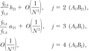
, number and type of mutations involved. Thus the proba-bility that a segment of typei⫽ 1 (A1B1) in patchkis a mutant typej⬆ifrom the same patch is

equilibrium frequencies do not matter greatly (we as-sume that selection is completely symmetric so that the sizes of the two allelic classes,A1andA2, are even), but the assumption that there is no subdivision does, as we yˆ2,k

yˆ1,k

b21⫹ O

冢

1

N2

冣

, j⫽ 2 (A1B21),

yˆ3,k

yˆ1,k

a21⫹O

冢

1

N2

冣

, j⫽ 3 (A2B1),

O

冢

1

N2

冣

, j⫽ 4 (A2B2),

see later. We also assume mutation between the two allelic classes is rare and symmetric (i.e.,A1mutates to A2at the same rate asA2mutates toA1). This assumption is discussed further below as well.

(7)

Figure 2 shows a typical realization of this model. The for example. The recombination probabilities depend

time to the most recent common ancestor (MRCA) of on the genotype in which the recombination event

the sample is extremely high at the selected site and would have taken place. Recombination in homozygotes

decreases with distance. The reason for this is clear: The or single heterozygotes can be treated as in the

single-selected site itself cannot coalesce unless a mutation locus model, but recombination in double

heterozy-from one allelic class to the other occurs. Since muta-gotes cannot. Consider again a segment of type i ⫽ 1

tions are rare, this means that, almost always, all mem-(A1B1) in patchk. The probability that it is a recombinant

bers of a particular class will coalesce to the MRCA of from an {1,j} individual in the same patch is

that class long before a mutation occurs. Sites that are more distantly linked to the selected site can move be-yˆj,kr⫹O

冢

1

N2

冣

, (8)

tween allelic classes by recombination and coalesce much faster.

forj ⫽1, 2, 3. However, it can also be a recombinant

The genealogical pattern shown in Figure 2 may result from a {1, 4} individual (thecis-heterozygote,A1B1/A2B2),

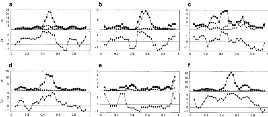
in a characteristic pattern of polymorphism, which may as long as the recombination did not take place between the

be detected in the data. Figure 3 shows the distribution two loci. The probability of this event is thus

of the amount of variation within and between allelic classes and of Tajima’sDstatistic along the chromosome yˆ4,k(1⫺d)r⫹O

冢

1

N2

冣

. (9) _{in six realizations. It is evident that the presence of} balancing selection usually causes a “peak” due to diver-Given such an event, the breakpoint can be anywhere in _{gence between the two allelic classes. This well-known} the flanking pieces (it could, for example, be uniformly _{phenomenon is also reflected in Tajima’s}

D, which is distributed). The opposite is true if the segment is a _{expected to be greater than zero in the presence of} recombinant from a {2, 3} individual (thetrans-heterozy- _{balancing selection or (many forms of) population} sub-gote,A1B2/A2B1), because in this case the recombination _{division (Tajima1989). However, note the considerable} must have taken place between the loci. The probability _{randomness: The peaks are not always centered on the}

of this is _{selected site; in Figure 3b, variation is inflated within}

one of the allelic classes as well as between them; and yˆ2,kyˆ3,k

yˆ1,k

dr⫹O

冢

1

N2

冣

. (10) in Figure 3e, there is no peak at all. The pattern of polymorphism depends heavily on the history of muta-All other events have probabilityO(1/N2_{) or less.}

tions between the allelic classes, as well as on the history The extension to nsegments and the conversion to _{of recombination in the region.}

continuous time can be done precisely as for the single- _{We considered the power to detect selection using} locus model. The complete transition rates are given in _{Tajima’sDstatistic. Table 2 gives the probability of}

ob-Table 1. _{serving a significantly positive value of this statistic under}

various assumptions. Several conclusions are clear. First, the power depends sensitively on the width of the win-DETECTING SELECTION

dow used to calculate D. A very small window will not have enough segregating sites to achieve statistical sig-In this section we use simulations to investigate the

distribution of the pattern of polymorphism in regions nificance, whereas a large window will “drown” the peak in neutral noise. The optimal window width will depend that contain sites subject to balancing polymorphism.

We are in particular interested in the power to detect on the ratio between␪and␳,i.e., the number of neutral mutations per recombination. If ␪/␳ ⬎ 1, balancing selection under various models and assumptions about

parameter values. The simulation software, which is writ- selection should usually be detected, but if␪/␳ Ⰶ1, it usually will not be.

ten in C⫹⫹with a Mathematica front end, is available

on request. To make the numbers in Table 2 applicable to

se-quence data, it is necessary to make assumptions about

Symmetric single-locus model:Consider first a

“classi-cal” balancing selection model, in which selection main- ␪ and␳ per base. Assume that ␪ ⫽ 0.01 per site, as is reasonable for Drosophila melanogaster (Przeworski et tains two different alleles at high frequencies in a

TABLE 1

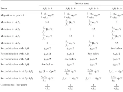
Backward transition rates in the two-locus model

Present state

Event A1B1ink A1B2ink A2B1ink A2B2ink

Migration to patchl 1

2

clyˆ1,l

ckyˆ1,k

φlk/2

1 2

clyˆ2,l

ckyˆ2,k

φlk/2

1 2

clyˆ3,l

ckyˆ3,k

φlk/2

1 2

clyˆ4,l

ckyˆ4,k

φlk/2

Mutation toA1B1 NA

yˆ1,k

yˆ2,k

␤12/2

yˆ1,k

yˆ3,k

␣12/2 0

Mutation toA1B2

yˆ2,k

yˆ1,k

␤21/2 0 NA

yˆ2,k

yˆ4,k

␣12/2 Mutation toA2B1

yˆ3,k

yˆ1,k

␣21/2 NA 0

yˆ3,k

yˆ4,k

␤12/2

Mutation toA2B2 0

yˆ4,k

yˆ2,k

␣21/2

yˆ4,k

yˆ3,k

␤21/2 NA

Recombination withA1B1 yˆ1,k␳/2 yˆ1,k␳/2 yˆ1,k␳/2 See below

Recombination withA1B2 yˆ2,k␳/2 yˆ2,k␳/2 See below yˆ2,k␳/2

Recombination withA2B1 yˆ3,k␳/2 See below yˆ3,k␳/2 yˆ3,k␳/2

Recombination withA2B2 See below yˆ4,k␳/2 yˆ4,k␳/2 yˆ4,k␳/2

Recombination inA1B1/A2B2 yˆ4,k(1⫺d)␳/2

yˆ1,kyˆ4,k

yˆ2,k

d␳/2 yˆ1,ky4,k

yˆ3,k

d␳/2 yˆ1,k(1⫺d)␳/2

Recombination inA1B2/A2B1

yˆ2,kyˆ3,k

yˆ1,k

d␳/2 yˆ3,k(1⫺d)␳/2 yˆ2,k(1⫺d)␳/2

yˆ2,kyˆ3,k

yˆ4,k

d␳/2

Coalescence (per pair) 1

ckyˆ1,k

1

ckyˆ2,k

1

ckyˆ3,k

1

ckyˆ4,k

NA, not applicable.

Table 2 correspond to 1 kb, and the optimal window ing selection, it is no longer reasonable to assume that each site is hit only once. Depending on the level of size is usually 100 bp. Balancing selection affects very

small regions. This realization calls into question the selective constraint, at most 1000 selectively neutral sites are in the region, and more likely 1000/3. When finite infinite-sites assumption for mutation, because, given

the very long coalescence times expected under balanc- sites are taken into account, balancing selection

Figure3.—Sliding-window analysis of the distribution of the average number of pairwise differences within and between the two different allelic classes (␲wand␲b, respectively) and of Tajima’s Din six realizations of the symmetric balancing selection model described in the text. In the top, diamonds and stars connected by broken lines show the distributions of␲wfor the two allelic classes, and squares connected by solid lines show the distribution of␲b. The bottom shows the distribution of Tajima’s D. Simulations were carried out withn⫽24 (12 inA1and 12 inA2) and the infinite-sites recombination/mutation model with

␪ ⫽ ␳ ⫽10. A sliding-window of size 0.1 was moved with increments of 0.025.

comes harder to detect, because some of the “excess” that the mutation rate per base pair is 0.01, while the rate of back mutation would still be 0.01), there is usually variability simply results in repeat mutations (Table 2).

Loss-of-function mutations:Many cases of balancing no ancient polymorphism, and no peak of

polymor-phism will develop. As is illustrated in Table 2, balancing selection, especially those that are due to a trade-off

between resistance and cost of resistance to some para- selection is not likely to be detected in these cases. We return to this topic in thediscussion.

site or pathogen, are likely to involve loss-of-function

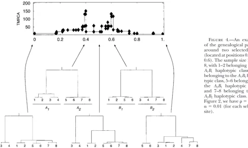
mutations (Olson 1999;Stahlet al. 1999; Johanson Two loci: Figure 4 shows a typical realization of a classical symmetric two-locus model with all four haplo-et al.2000; Tianet al.2002). This type of scenario fits

well into the modeling framework presented here, but types present at equal frequencies. The two selected sites are positioned at 0.4 and 0.6, respectively. Note leads to very different predictions. Specifically, since

mutation between the two allelic classes is essentially that the topologies of the trees behave in the intuitively obvious way as we walk along the chromosome: Close unidirectional (for example, if mutation at any of 100

different sites can lead to loss of function, then the total to each selected site, the sample must coalesce in a manner determined by the allelic classesat that site. In rate of loss-of-function mutations would be 1, assuming

TABLE 2

The probability (%) of detecting balancing selection

Width of window

Infinite sites Finite sites (1000 bp) Finite sites (333 bp)

␳ 0.025 0.05 0.1 0.2 1 0.025 0.05 0.1 0.2 1 0.025 0.05 0.1 0.2 1

1 88.1 91.4 93.3 94.3 88.2 85.6 90.2 92.8 93.5 83.8 75.0 83.8 89.4 91.5 76.5

3 84.7 88.2 88.9 87.1 57.6 80.8 85.3 86.3 83.5 44.7 69.2 76.6 79.2 76.4 32.2

10 76.7 77.3 73.6 62.0 7.7 69.0 69.9 64.5 51.0 4.1 55.2 57.6 52.3 39.9 2.4

30 59.3 53.2 40.7 22.0 0.2 48.1 42.5 31.0 15.7 0.1 37.2 34.3 23.8 11.5 0.0

100 26.0 20.2 10.9 3.1 0.0 20.5 15.6 8.9 2.4 0.0 15.4 12.3 6.9 2.1 0.0

10a _{3.7 6.1 6.8 5.2 0.3 3.7 6.0 6.8 5.1 0.3 3.2 5.6 6.8 5.1 0.2}

Power was estimated from 5000 replicates (1000 for␳ ⫽100) using␪ ⫽10 andn⫽24 (12 in each allelic class). Selection was deemed to have been detected ifD⬎2.01 (Tajima1989) in a window of the specified size. In the finite-sites models, infinite-sites mutations (i.e., random numbers in the unit interval) that were sufficiently close to each other were deemed to have affected the same site and simply reverted it to its previous state.

Figure 4.—An example of the genealogical pattern around two selected sites (located at positions 0.4 and 0.6). The sample size isn⫽

8, with 1–2 belonging to the

A1B1 haplotypic class, 3–4 belonging to theA1B2 haplo-typic class, 5–6 belonging to the A2B1 haplotypic class, and 7–8 belonging to the

A2B2haplotypic class. As in Figure 2, we have␳ ⫽2 and

␣ ⫽0.01 (for each selected site).

a sample that contains the “complementary” haplotypes (not shown). Obviously, the best strategy is to use a window size that captures each peak, but since the num-(A1B1andA2B2orA1B2andA1B2), sites located between

the selected sites can coalesce only if there are at least ber of selected sites is not knowna priori, this may be difficult to implement in practice. However, regions con-two recombination events.

Figure 5 illustrates the effect of the distance between taining multiple sites subject to balancing selection are considerably less likely to be missed (see alsoNavarro

the selected sites on the distribution of␲w,␲b, and

Taji-ma’sDalong the chromosome. If the distance between andBarton2002).

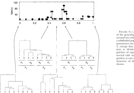
Subdivision: The behavior of balancing selection

the sites is sufficiently great, there may be two distinct

peaks (Figure 5, a and b); otherwise, only a single peak models with population subdivision is very complicated, but the example shown in Figure 6 illustrates the main may be visible (Figure 5c). Power studies analogous to

those in Table 2 indicate that the probability of rejecting points. In addition to the structure imposed by the al-lelic and haplotypic classes, there is now population neutrality using Tajima’sDdepends sensitively on the

positioning, numbers, and sizes of the windows used structure as well. Which structure turns out to be

Figure 6.—An example of the genealogical pattern around two selected sites in a subdivided population. The parameters are as in Figure 4, except that the popula-tion is divided into two patches of equal size, con-nected with symmetric mi-gration at rateφ⫽0.1. The structure of the sample is shown.

dominant will depend on the relative magnitudes of lated region, completely obscuring the peak around the B-locus. Multiple linked sites involved in local adapta-the parameters. In adapta-the example shown in Figure 6, adapta-the

pattern of coalescence differs between the two selected tion can, in principle, “lock up” entire chromosomal regions in complementary haplotypes.

sites. At the B-locus (located at 0.6), the first stage of coalescence is within allelic class within patches, fol-lowed by coalescence within allelic class between the

DISCUSSION two patches. Finally coalescence occurs between two

allelic classes. On the other hand, at theA-locus (located We have shown how the “structured coalescent” de-scribed by Nordborg (1997) may be combined with at 0.4), there is a cluster of the four sequences in patch

2, and the longest branch is between sequence 1 (A1in the “ancestral recombination graph” ofGriffithsand

Marjoram (1997) to yield a genealogical model for

patch 1) and the others. The genealogical pattern is

highly variable between realizations. sequences that contain multiple sites subject to strong selection in a subdivided population. We refer to the

Local adaptation: An important motivation for the

model described above is to consider local adaptation. combined model as the “structured ancestral recombi-nation graph” (SARG). Albeit complex, the SARG is A balance between migration and selection seems much

more likely to maintain polymorphism than does “pure” highly suitable for simulation, just like the standard coalescent.

balancing selection. Because local adaptation leads to

a deficit of heterozygotes at the selected locus or loci, Robustness of the SARG:We described the SARG as a limiting approximation to a specific model of pollen the effect on linked neutral variation may be much

greater. Local adaptation should thus be much easier flow in an outcrossing hermaphroditic plant species, but the SARG is much more general. As is the case for to detect using polymorphism data.

Figure 7 shows an example of a single-locus model the standard coalescent, phenomena such as selfing, separate sexes, or sex linkage, etc., can readily be incor-of local adaptation. The frequency incor-ofA1is assumed to

be 0.9 in patch 1 and 0.1 in patch 2 (and conversely porated (although formally proving convergence is likely to be both difficult and tedious; see Nordborg

for A2). The effects of local adaptation are even more

dramatic when multiple sites are involved. Figure 8 andKrone2002).

The hardest problem from a mathematical point of shows an example of a two-locus model where A1B1 is

simu-Figure 7.—An example of the genealogical pattern around a site involved in lo-cal adaptation (located at position 0.5). The selected site is located at position 0.5. The two equal-sized patches are connected with symmetric migration at rate

φ⫽0.1; the rest of the pa-rameters are as in Figure 2. The sample size is n ⫽ 8, with 1–3 belonging to A1 and 4 belonging to A2 in patch 1, and 5 belonging to

A1and 6–8 belonging toA2 in patch 2.

as population structure? For strong balancing selection, the adaptively important sites. This may be the case in strong clines and even in some hybrid zones (although it is plausible to argue that the approximation is a good

one (Kaplanet al.1988). In particular, when local adap- the approximation will certainly break down if the num-ber of selected loci becomes too large; seeBartonand tation is involved, it is easy to imagine very strong

selec-tion. However, to treat allele frequencies as constant in Navarro2002).

Detecting balancing selection:Our motivation for

de-a model of locde-al de-adde-aptde-ation, it is de-also necessde-ary to de-assume

that migration is strong so that a deterministic migra- riving the SARG was that we wanted to simulate se-quence data from regions containing sites subject to tion-selection balance results. In such a model, there

would be no signs of subdivision when looking at neutral balancing selection. It has long been known that balanc-ing selection may create a peak of increased polymor-markers unless these were sufficiently closely linked to

phism centered around the selected site (Hudsonand tions sufficiently for ancient polymorphism to be main-tained.

Kaplan1988). Numerous articles have been published

about theexpected levels of polymorphism surrounding _{We thank A. Navarro and an anonymous reviewer for comments} such a site (e.g.,Nordborget al.1996;KellyandWade on the manuscript. M.N. thanks Peter Donnelly, Bob Griffiths, Dick Hudson, Steve Krone, Tom Kurtz, Paul Marjoram, Claudia Neuhauser, 2000; Schierup et al. 2000; Barton and Navarro

Gesine Reinert, Simon Tavare´, and Carsten Wiuf for many, many 2002). These kinds of results are of limited value for

conversations about selection. data analysis, because the pattern of polymorphism

sur-rounding any particular balanced polymorphism will reflect the random history of this region and will usually

LITERATURE CITED be very far from expectations.

Using simulations, we have focused on the question Andolfatto, P., andM. Nordborg, 1998 The effect of gene conver-sion on intralocus associations. Genetics148:1397–1399. of whether we should expect balancing selection to be

Barton, N. H., andA. Navarro, 2002 Extending the coalescent to detectable or not. Our original motivation for asking _{multilocus systems: the case of balancing selection. Genet. Res.} this question is that many years of population genetics 79:129–139.

Braverman, J. M., R. R. Hudson, N. L. Kaplan, C. H. Langleyand research in Drosophila have failed to uncover strong

W. Stephan, 1995 The hitchhiking effect on the site frequency evidence for balancing selection. Is this because balanc- _{spectrum of DNA polymorphism. Genetics140:783–796.} ing selection is indeed rare, perhaps limited to highly Campbell, R. B., 1999 The coalescent time in the presence of

back-ground fertility selection. Theor. Popul. Biol.55:260–269. unusual cases, like the MHC and plant

self-incompatibil-Donnelly, P., andT. G. Kurtz, 1999 Genealogical processes for ity loci (Kreitman and Akashi 1995;Hudson 1996), _{Fleming-Viot models with selection and recombination. Ann.} or is it simply very difficult to detect because recombina- Appl. Probab.9:1091–1148.

Fearnhead, P., 2001 Perfect simulation from population genetic tion and gene conversion effectively destroys the

evi-models with selection. Theor. Popul. Biol.59:263–279. dence (AndolfattoandNordborg1998)? The latter _{Griffiths, R. C., andP. Marjoram, 1997 An ancestral} recombina-view is supported by several recent observations of bal- tion graph, pp. 257–270 in Progress in Population Genetics and Human Evolution, edited by P.Donnellyand S.Tavare´. Springer-ancing selection in Arabidopsis thaliana (Stahl et al.

Verlag, New York.

1999;Tianet al.2002), where recombination is expected _{Hey, J., 1991 A dimensional coalescent process applied to} multi-to be less effective because of selfing (Nordborg1997). allelic selection models and migration models. Theor. Popul. Biol.

39:30–48. Our simulations also tend to support the view that

Hudson, R. R., 1996 Molecular population genetics of adaptation, balancing selection might be difficult to detect in out- _{pp. 291–309 inAdaptation, edited by M. R.Roseand G. V.Lauder.} crossing organisms. For␪/␳ ⫽1, as may be typical for Academic Press, San Diego.

Hudson, R. R., andN. L. Kaplan, 1988 The coalescent process in Drosophila, taking finite sites into account, power to

models with selection and recombination. Genetics120:831–840. detect balancing selection seems to be ⵑ50% (Table _{Hudson, R. R., andN. L. Kaplan, 1995 Deleterious background} 2). Note that this is power in the evolutionary sense, selection with recombination. Genetics141:1605–1617.

Hudson, R. R., K. Bailey, D. Skarecky, J. KwiatowskiandF. J.

not in the usual “sampling” sense: It is not the case that

Ayala, 1994 Evidence for positive selection in the superoxide a different sample would detect balancing selection; _{dismutase (Sod) region ofDrosophila melanogaster.Genetics136:} rather it is the case that a large fraction of existing 1329–1340.

Innan, H., and F. Tajima, 1999 The effect of selection on the balancing polymorphisms are expected to be

undetect-amounts of nucleotide variation within and between allelic able (because of the particular evolutionary history of _{classes. Genet. Res.73:15–28.}

the polymorphism). Power will of course also depend Johanson, U., J. West, C. Lister, S. Michaels, R. Amasinoet al., 2000 Molecular analysis ofFRIGIDA, a major determinant of on sampling and on the statistical method used, but

natural variation inArabidopsisflowering time. Science290:344– perhaps less than we would think. It should be noted _347.

that our simulations do not take gene conversion into Kaplan, N. L., T. DardenandR. R. Hudson, 1988 The coalescent process in models with selection. Genetics120:819–829. account: This could decrease power further (

Andol-Kaplan, N. L., R. R. HudsonandC. H. Langley, 1989 The

“hitch-fattoandNordborg1998). _{hiking” effect revisited. Genetics123:887–899.}

Finally, it seems clear that we should not normally Kaplan, N. L., R. R. HudsonandM. Iizuka, 1991 The coalescent process in models with selection, recombination and geographic expect to be able to see a typical signal of balancing

subdivision. Genet. Res.57:83–91.

selection when selection maintains a polymorphism be- _{Kelly, J. K., andM. J. Wade, 2000 Molecular evolution near a} two-tween loss-of-function and functional alleles. The reason locus balanced polymorphism. J. Theor. Biol.204:83–101.

Kim, Y., andW. Stephan, 2002 Detecting a local signature of genetic is simply that loss-of-function alleles are created far too

hitchhiking along a recombining chromosome. Genetics160:

rapidly to be ancient. When loss-of-function alleles

765–777.

nonetheless appear to be ancient, as is the case for some Kreitman, M., andH. Akashi, 1995 Molecular evidence for natural selection. Annu. Rev. Ecol. Syst.26:403–422.

disease-resistance loci inA. thaliana(Stahlet al.1999;

Krone, S. M., andC. Neuhauser, 1997 Ancestral processes with

Tianet al.2002), this may be an indication that not all

selection. Theor. Popul. Biol.51:210–237.

loss-of-function alleles are created equal: It is notable _{Navarro, A., andN. H. Barton, 2002 The effects of multilocus} balancing selection on neutral variability. Genetics161:849–863. that these cases involve complete deletions, and it may

Neuhauser, C., 1999 The ancestral graph and gene genealogy un-be that such deletions are preferable to point mutations

der frequency-dependent selection. Theor. Popul. Biol.56:203– that may lead to incorrectly folded proteins, for exam- _214.

muta-pp. 153–178 in Handbook of Statistical Genetics, edited by D. J. Schierup, M. H., D. CharlesworthandX. Vekemans, 2000 The effect of hitch-hiking on genes linked to a balanced

polymor-Balding, M. J.Bishopand C.Cannings. John Wiley & Sons,

Chichester, UK. phism in a subdivided population. Genet. Res.76:63–73.

Schierup, M. H., A. M. MikkelsenandJ. Hein, 2001

Recombina-Neuhauser, C., andS. M. Krone, 1997 The genealogy of samples

in models with selection. Genetics145:519–534. tion, balancing selection and phylogenies in MHC and self-incom-patibility genes. Genes159:1833–1844.

Nordborg, M., 1997 Structured coalescent processes on different

time scales. Genetics146:1501–1514. Simonsen, K. L., G. A. ChurchillandC. F. Aquadro, 1995 Proper-ties of statistical tests of neutrality for DNA polymorphism data.

Nordborg, M., 1999 The coalescent with partial selfing and

balanc-ing selection: an application of structured coalescent processes, Genetics141:413–429.

Slade, P. F., 2000a Most recent common ancestor probability distri-pp. 56–76 inStatistics in Molecular Biology and Genetics(IMS Lecture

Notes-Monograph Series, Vol. 33), edited by F.Seillier-Moisei- butions in gene genealogies under selection. Theor. Popul. Biol.

58:291–305.

witsch. Institute of Mathematical Statistics, Hayward, CA.

Nordborg, M., 2001 Coalescent theory, pp. 179–212 inHandbook Slade, P. F., 2000b Simulation of selected genealogies. Theor. Popul. Biol.57:35–49.

of Statistical Genetics, edited by D. J.Balding, M. J.Bishopand

C.Cannings. John Wiley & Sons, Chichester, UK. Slade, P. F., 2001 Simulation of “hitch-hiking” genealogies. J. Math. Biol.42:41–70.

Nordborg, M., andS. M. Krone,2002 Separation of time scales

and convergence to the coalescent in structured populations, pp. Stahl, E. A., G. Dwyer, R. Mauricio, M. KreitmanandJ. Bergel-son, 1999 Dynamics of disease resistance at theRpm1locus of 194–232 inModern Developments in Theoretical Population Genetics:

The Legacy of Gustave Male´cot, edited by M. Slatkin and M. Arabidopsis.Nature400:667–671.

Tajima, F., 1989 Statistical method for testing the neutral mutation

Veuille. Oxford University Press, Oxford.

Nordborg, M., B. Charlesworthand D. Charlesworth, 1996 hypothesis by DNA polymorphism. Genetics123:585–595. Increased levels of polymorphism surrounding selectively main- Takahata, N., 1990 A simple genealogical structure of strongly tained sites in highly selfing species. Proc. R. Soc. Lond. Ser. B balanced allelic lines and trans-species polymorphism. Proc. Natl.

263:1033–1039. Acad. Sci. USA87:2419–2423.

Olson, M. V., 1999 When less is more: gene loss as an engine of Takahata, N., andY. Satta, 1998 Footprints of intragenic recombi-evolutionary change. Am. J. Hum. Genet.64:18–23. nation at HLA loci. Immunogenetics47:430–441.

Przeworski, M., 2002 The signature of positive selection at ran- Tian, D., H. Araki, E. Stahl, J. BergelsonandM. Kreitman, 2002 domly chosen loci. Genetics160:1179–1189. Signature of balancing selection inArabidopsis.Proc. Natl. Acad.

Przeworski, M., J. D. WallandP. Andolfatto, 2001 Recombina- _{Sci. USA99:11525–11530.} tion and the frequency spectrum inDrosophila melanogasterand