The Advantages of Segregation and the Evolution of Sex



The Advantages of Segregation and the Evolution of Sex

Sarah P. Otto

Department of Zoology, University of British Columbia, Vancouver, British Columbia V6T 1Z4, Canada Manuscript received October 28, 2002

Accepted for publication February 18, 2003

ABSTRACT

In diploids, sexual reproduction promotes both the segregation of alleles at the same locus and the recombination of alleles at different loci. This article is the first to investigate the possibility that sex might have evolved and been maintained to promote segregation, using a model that incorporates both a general selection regime and modifier alleles that alter an individual’s allocation to sexualvs.asexual reproduction. The fate of different modifier alleles was found to depend strongly on the strength of selection at fitness loci and on the presence of inbreeding among individuals undergoing sexual reproduction. When selection is weak and mating occurs randomly among sexually produced gametes, reductions in the occurrence of sex are favored, but the genome-wide strength of selection is extremely small. In contrast, when selection is weak and some inbreeding occurs among gametes, increased allocation to sexual reproduction is expected as long as deleterious mutations are partially recessive and/or beneficial mutations are partially dominant. Under strong selection, the conditions under which increased allocation to sex evolves are reversed. Because deleterious mutations are typically considered to be partially recessive and weakly selected and because most populations exhibit some degree of inbreeding, this model predicts that higher frequencies of sex would evolve and be maintained as a consequence of the effects of segregation. Even with low levels of inbreeding, selection is stronger on a modifier that promotes segregation than on a modifier that promotes recombination, suggesting that the benefits of segregation are more likely than the benefits of recombina-tion to have driven the evolurecombina-tion of sexual reproducrecombina-tion in diploids.

S

evolu-otes (Bell1982), but why sex evolved and why it tion and maintenance of genetic mixing in the face of is maintained in so many species have remained un- environmental change, mutation, and drift (see reviews

resolved questions in evolutionary biology. Paradoxically, by Barton and Charlesworth 1998; Otto and

sexual reproduction, while common, entails several costs Michalakis1998;Westet al.1999;Ottoand Lenor-that are avoided by asexuals. Sexual organisms must find mand2002), but these studies have largely ignored ge-and court a mate, must risk disease transmission ge-and netic associations within a locus under the assumption predation during mating, and are prone to conflicts that sex evolved to promote recombination among al-between the sexes, including conflicts over parental care leles at different loci. Furthermore, those theoretical (e.g., a partner may contribute few resources to offspring models investigating the evolution of rates of genetic production;Maynard Smith1978) and conflicts over mixing within a population (so-called “modifier mod-investment in currentvs. future reproduction (Moore els”) have focused almost exclusively on the evolution andHaig1991;Chapmanet al.1995). A further prob- of recombination rates. Yet sex entails the segregation lem with sexual reproduction is that it breaks up genetic of alleles at each locus as well as recombination between associations that have accumulated over time in re- alleles at different loci. Just as recombination breaks up sponse to selection. In a constant environment without _{genetic associations among loci (linkage disequilibria),} mutations or genetic drift, these genetic associations _{segregation breaks up genetic associations within a locus} are typically favorable, and theoretical analyses have _{(departures from Hardy-Weinberg proportions). Thus,} demonstrated that decreased levels of recombination _{selection could indirectly favor the evolution of sexual} evolve under such circumstances (Feldman1972;Alten- _{reproduction through the effects of sex on one-locus} berg and Feldman 1987; Feldman et al. 1997). The _{genetic associations. Using a model that allows the} allo-resolution to the paradox of sex must, therefore, lie _{cation to asexualvs.sexual reproduction to depend on} with perturbations—resulting from biotic or abiotic _{a modifier locus, this article investigates when we would} changes in the external environment, mutation, and/ _{expect increased sex to evolve as a consequence of}

segre-or random genetic drift within a population. _{gation rather than recombination.}

Within a randomly mating diploid species, sexual re-production (meiosis followed by syngamy) breaks down

1_{Address for correspondence:Department of Zoology, 6270 University}

associations between alleles carried on homologous chro-Blvd., University of British Columbia, Vancouver, BC V6T 1Z4, Canada.

E-mail: [email protected] mosomes at a locus. Indeed, within a large, fully sexual

population exhibiting nonoverlapping generations, ge- pared to an asexual population (Crow1970;Peckand Waxman2000).

netic associations at a locus are completely eliminated

and Hardy-Weinberg proportions are attained after one Second, consider purifying selection acting against mutant alleles at a locus. Within a population containing generation of random mating. Within asexual

popula-tions or partially sexual populapopula-tions, however, one-locus both wild-type (A) and mutant (a) alleles, the relative fitness of a diploid individual can be written as genetic associations can persist and accumulate over

time. Whenever these genetic associations affect fitness,

Fitness(AA)⫽1, Fitness(Aa)⫽1⫺hs, Fitness(aa)⫽1⫺s, indirect selection will act on any feature that alters their

(2a) accumulation, including the level of sexual

reproduc-tion. Genetic associations between two alleles (Aanda) wheresis the selection coefficient (0⬍sⱕ1) andhis at a locus (A) are typically measured by the inbreeding the dominance coefficient (0ⱕhⱕ1). The dominance

coefficient,F, as coefficient, h, measures one-locus fitness interactions

on an additive scale. An alternative coefficient that plays a more central role in the evolution of sex measures F⫽ pAA⫺ p

2 A

pApa _{dominance on a multiplicative scale:}

␫ ⫽Fitness(AA)Fitness(aa)⫺Fitness(Aa)2 ⫽ pAApaa ⫺(pAa/2)2

pApa

, (1)

⫽ ⫺s(1⫺2h⫹ h2_{s). (2b)} wherepijandpkare the frequencies of genotypeijand

On a log scale, ␫ measures whether homozygotes are allelek. As indicated by the first part of Equation 1,F

more fit (␫ ⬎0) or less fit (␫ ⬍0) than expected based measures the difference between the observed

fre-on the fitness of heterozygotes. Note that ␫ can be quency of a genotype and its expected frequency at

thought of as a one-locus analog of epistasis (ε), which Hardy-Weinberg equilibrium. As indicated by the

sec-is a measure of fitness interactions between alleles at ond part of Equation 1,Falso measures whether

homo-two loci (seecomparisons to other models and in-zygotes are more frequent (F ⬎ 0) or less frequent

terpretation). If mutations recur at frequency␮per (F⬍0) than expected based on the frequency of

heter-gamete per generation and if mating is random among ozygotes within the population. Thus,Fcan be thought

individuals reproducing sexually, the equilibrium fre-of as a one-locus analog fre-of the gametic-phase linkage

quency of Aa individuals isⵑ2␮/(hs) in both asexual disequilibrium (D), which measures whether

combina-and sexual diploid populations (assuming weak muta-tions of alleles at two loci are more or less frequent than

tion, ␮ Ⰶ hs). The mean fitness is then ⵑ1 ⫺ 2␮. A expected (seecomparisons to other models and

in-more exact treatment that keeps track of order␮2_terms terpretation). While F is called an “inbreeding

co-(Chasnov2000) indicates, however, that a negative ge-efficient,” processes besides inbreeding can generate

netic association (F) develops whenever departures from F ⫽ 0, including selection and drift.

While the associations between alleles at a locus gener- _{␫ ⬍0 (3a)}

ated by selection and drift would not persist in a fully

or, equivalently, sexual population, they do persist in a population that

reproduces asexually as well as sexually.

h⬍ 1

1⫹

√

With one exception (UyenoyamaandBengtsson1989, discussed below), all previous models that have

investi-gated the importance of segregation to the evolution Thus, when homozygotes are relatively less fit (␫ ⬍0), a departure from Hardy-Weinberg develops such that of sex have focused on mean fitness comparisons of

sexual and asexual populations rather than examining there are fewer homozygotes than expected at equilib-rium (F⬍0). This one-locus genetic association reduces the conditions under which sex evolves within a

popula-tion. Let us begin by reviewing these mean fitness re- the genetic variance in fitness, which hinders selection and slightly reduces the mean fitness at equilibrium. sults, focusing on the three main forms of selection at

a locus (heterozygote advantage, purifying selection, Segregation breaks down this detrimental association, causing sexual populations to have a slightly higher and directional selection). First, consider heterozygote

advantage. Within an asexual population, the frequency mean fitness than asexual populations at equilibrium (Chasnov 2000). Conversely, when homozygotes are of heterozygotes would rise to fixation, at which point

there would be a strong negative one-locus genetic asso- relatively more fit (␫ ⬎0), homozygotes become more common then expected (F⬎0), which slightly increases ciation (F⫽ ⫺1). Within a sexual population, however,

the segregation of alleles would break down the genetic genetic variance in fitness and the mean fitness at equi-librium. Now, the one-locus genetic associations built association, and the less fit homozygotes would be

formed by syngamy each generation. Hence, at equilib- up by selection are favorable. Consequently, the mean fitness at equilibrium is higher in asexual populations, rium, a sexual population would suffer a decrease in

popula-tions. Typically, data on dominance suggest that delete- To fully understand the evolution of sex, however, we must also ask how the frequency of sex evolves within rious mutations are partially recessive (h⬍1_⁄

2;Simmons

a population that is capable of both sexual and asexual

and Crow 1977; Deng and Lynch 1997;

Garcia-reproduction, as is common among protists, fungi, algae, Doradoet al.1999). Thus, we expect (3) to hold and

plants, and several invertebrate animal groups (Bell predict that sexual populations should have a higher

1982). This article addresses this question by tracking equilibrium mean fitness than asexual populations. As

the frequency of alleles that modify the relative alloca-long as sex involves random mating, this advantage is

tion to the two modes of reproduction within a single negligibly small unless deleterious mutations are very

population. Alleles at such a “modifier” locus (M) could recessive (␮/sⱕhⱕ

√

sex-act in any number of ways; for example, they could alter ual reproduction is accompanied by inbreeding (the

the probability of undergoing mitotic vs. meiotic cell union of gametes that are closely related by descent),

division in unicellular organisms or alter the probability however, homozygotes become more common than

ex-of reproducing via fission, budding, or apomixis in multi-pected at Hardy-Weinberg equilibrium, causing the

cellular organisms. mean fitness of sexual populations to be substantially

In this article, evolution at the modifier locus is exam-higher than that of asexual populations (Agrawaland

ined with respect to the dynamics at a locus,A, subject to Chasnov2001).

either purifying or directional selection, which exhibit Third, consider directional selection causing the

qualitatively similar results. For want of a better term, spread of a favored allele, A, within a population.

Al-theAlocus is called a “fitness locus.” In a companion though it is nonstandard, I continue to use the fitness

article, we examine the evolution of sex when the fitness regime described by (2) as this makes it easier to

recog-locus is subject to heterozygote advantage (Dolginand nize parallels between the results with purifying and

Otto2003, this issue), where, to our surprise, we also directional selection. The arguments made in the

previ-found that a modifier that increases the frequency of ous paragraph continue to apply when genetic

associa-sex can spread under reasonable sets of parameters. A tions are initially absent but are generated by directional

similar model was analyzed byUyenoyamaand Bengts-selection. That is, if (3) holds, selection will cause

homo-son(1989), although they restricted their attention to zygotes to become less common than expected,

decreas-lethal deleterious mutations; their results are summa-ing the genetic variance and slowsumma-ing down adaptive

rized where parallels exist to this article. As we shall evolution. By breaking down the one-locus genetic

asso-see, evolutionary change at the modifier locus depends ciations, sexual reproduction speeds up selection and

strongly on the degree of inbreeding within the popula-gains a long-term advantage. Conversely, if (3) fails to

tion and the degree of dominance and strength of selec-hold, selection generates excess homozygosity, a genetic

tion at fitness loci. I argue that, for biologically reason-association that hastens adaptive evolution. Now, by

able values of these parameters, selection generally breaking down the associations, sexual reproduction

favors the evolution of increased levels of sexual repro-hinders selection and suffers a long-term disadvantage.

duction and that such selection is strong relative to other This argument assumes that all genotypes are initially

deterministic forces acting on the evolution of sex. present. Imagine instead thatAarises as a single

muta-tion in a heterozygous individual. The spread of the favorable allele would then be limited to the fixation

MODEL

of the heterozygote within asexual populations, at which

point adaptive evolution would stall until theAAhomo- Consider two loci, a modifier locus Mand a fitness zygote was generated by a second mutation or mitotic locus A, within a diploid population with nonoverlap-recombination (Kirkpatrick and Jenkins 1989). In ping generations. To track changes in allele frequencies contrast, theAAhomozygote would be produced imme- at these loci, we begin by censusing at the juvenile stage, diately by segregation within sexual populations, has- before selection, and then proceed through selection, tening adaptation and providing sexual populations mutation, and reproduction. Letxijequal the frequency

with a long-term fitness advantage over asexual popula- of juveniles that carry haplotypesi andj(wherei and

tions (KirkpatrickandJenkins1989). jequal 1 for haplotype MA, 2 forMa, 3 formA, and 4

The above discussion focuses on the effects of selec- forma). I assume that all loci are autosomal, that selec-tion on one-locus genetic associaselec-tions (F) and long-term tion does not depend on the sex of the parent, and that mean fitness within an asexual population or a sexual there is no selection at the haploid or gametic stage. population. These results can predict the outcome of Consequently, I assume thatxij ⫽xji and keep track of

competition between sexual and asexual populations, xij forjⱖ i, only. Thus, for example, the frequency of

but only if the sexual and asexual populations are eco- MM AAindividuals is x11but the frequency ofMM Aa logically equivalent yet have been reproductively iso- individuals is 2x12. At this point, selection occurs ac-lated for long enough for genotypes to reach the fre- cording to Equation 2. Letx˜ijequal the frequency after

x˜11⫽x11/W⫽ Frequency(MM AA) loids of genotypeijwith probabilityyiyj. Inbreeding

oc-curs among the gametes of a haploid gametophyte, after selection

resulting in the production of genotypeiifrom haploids of genotypeiwith probabilityyi. I refer to this form of

2x˜12⫽2x12(1⫺ hs)/W⫽ Frequency(MM Aa)

inbreeding as gametophytic selfing (this corresponds to after selection,

“intragametophytic selfing” in the terminology of Kle-kowski1969). Gametophytic selfing is only one mecha-etc., whereWis the mean fitness within the population.

nism by which inbreeding can occur. Inbreeding also At this stage, mutations from alleleAtoaoccur at rate

occurs when there is sporophytic selfing (where the ␮, regardless of the mode of reproduction. Mutations

gametes of a diploid adult are mixed at random), mating from alleleatoAmay also occur, but they are ignored

among kin, and/or spatial population structure. It is because, at mutation-selection balance, alleleais so rare

important to keep in mind that the rate of inbreeding that the frequency of revertants toAis vanishingly small.

(f) is a measure of who mates with whom, whereas the In the case of a favorable allele spreading through a

population, mutations assert a very small influence on inbreeding coefficient (F) measures a departure from the dynamics and are ignored. Let x˜˜ij equal the geno- Hardy-Weinberg proportions regardless of the cause of

type frequencies after selection and mutation, where this departure. While all forms of inbreeding generate an excess of homozygosity (positiveF), gametophytic

self-x˜˜11⫽(1⫺ ␮)2x˜11⫽Frequency(MM AA)

ing does this to the greatest degree (100% of offspring

after mutation and selection,

are homozygous). Nevertheless, it is expected that

quali-2x˜˜12⫽2(1⫺ ␮)x˜12⫹2␮(1⫺ ␮)x˜11⫽Frequency(MM Aa)

tatively similar results to the current model would be

after mutation and selection,

observed with other mechanisms of inbreeding. The overall contribution to the juveniles of the next etc.

generation through sexual reproduction is then weighted At this point, reproduction occurs. The probability that

by the population’s average allocation to sex, ␴. Thus, an individual reproduces sexually depends on its

geno-the frequency ofMM AAjuveniles in the next generation type at the modifier locus,M:

equals

Genotype: MM Mm mm

x⬘11⫽ (1⫺ ␴1)x˜˜11⫹ ␴ (y21(1 ⫺f)⫹y1f), (6a)

Probability of sex: ␴1 ␴2 ␴3

and the frequency ofMM Aajuveniles (including both If an individual of genotypeijdoes not reproduce sexu- _{12 and 21 genotypes) in the next generation equals} ally, which occurs with probability 1⫺ ␴, then it

contrib-2x⬘12⫽(1⫺ ␴1)2x˜˜12⫹ ␴(2y1y2(1 ⫺f)). (6b) utes directly to the frequency of juveniles of genotype

ij in the next generation (x⬘ij). If the individual

repro-Recursion equations (6c)–(6j) for the remaining dip-duces sexually, meiosis occurs with recombination

be-loid juveniles were derived similarly (available upon re-tween the M andA loci at rate r. In many organisms

quest). Table 1 summarizes the notation. For the case with both sexual and asexual reproduction, including

ofs ⫽1, these recursions are identical to those devel-most sexual protists, fungi, algae, and nonseed plants,

oped byUyenoyamaandBengtsson(1989) when

in-sex involves an alternation of generations between

hap-breeding is absent (f⫽0) but differ when inbreeding is loid and diploid phases (Bell1982). I thus assume that

present, because they assume sporophytic selfing rather meiosis generates haploid gametophytes, among whom

than gametophytic selfing. the frequency of haplotypeiis given byyi. The frequency

Throughout the analyses, the recursions (6) are used ofMAhaploids, for example, would be

to determine when a modifier that increases the fre-quency of sex would spread within a population. To

y1⫽ ␴

1(x≈11⫹x≈12)⫹ ␴2(x≈13⫹x≈14(1⫺r)⫹x≈23r)

␴ , (4) begin, I analyze the case where the population is at a

mutation-selection balance at the Alocus with the M where␴is the average allocation of the diploid

popula-allele fixed at the modifier locus. I then determine the tion to sexual reproduction,

conditions under which a new modifier allele, m, can spread if it alters the level of sex within the population. ␴ ⫽ ␴1(x˜˜11⫹ 2x˜˜12⫹x˜˜22)⫹ ␴2(2x˜˜13⫹ 2x˜˜14

The results differ substantially depending on whether ⫹2x˜˜23⫹ 2x˜˜24)⫹ ␴3(x˜˜33⫹2x˜˜34⫹x˜˜44). (5)

or not there is inbreeding (i.e.,f⫽0 orf⬆0), so these cases are discussed in turn. Next, I turn to the case The haploid phase is assumed to be limited in scope,

of directional selection where a beneficial allele, A, is and selection in this phase is ignored. Genetically

identi-increasing in frequency within a population, assuming cal gametes are then produced by each haploid. The

that mutation is a negligible force. Finally, connections probability that any two gametes unite to form a zygote

are drawn between the results of this model of segrega-depends on the mating system. In this model, gametes

tion and models of recombination and ploidy evolution. undergo random union with probability 1 ⫺ f or

TABLE 1

Summary of notation

pA,pa Frequencies of the favorable (A) and deleterious (a) alleles at the fitness locusA

pM,pm Frequencies of the current (M) and new (m) alleles at the modifier locusM

F Inbreeding coefficient that measures excess homozygosity (Equation 1) D Linkage disequilibrium between two loci

s Selection coefficient acting against allelea(Equation 2)

h Dominance coefficient of alleleameasured on an additive scale (Equation 2)

␫ Dominance coefficient of alleleameasured on a multiplicative scale (⫽2hs⫺s⫺h2_s2₎

␮ Mutation rate from alleleAto alleleaper generation L Number of loci per genome

U Mutation rate to deleterious alleles per diploid genome per generation (⫽2␮L)

␴i Probability that a diploid reproduces sexually, wherei⫽1 forMM, 2 forMm, and 3 formm genotypes at the modifier locus

⌬␴ The homozygous effect of theMmodifier allele on the probability of sex (␴3⫺ ␴1) hM The dominance coefficient of theMmodifier allele (␴2⫽ ␴1⫹hM⌬␴)

␦␴ The allelic effect of an additive modifier (␴2⫽ ␴1⫹ ␦␴;␴3⫽ ␴1⫹2␦␴) f Selfing (inbreeding) rate among gametes (Equation 6)

r Recombination rate between lociAandM

xij Frequency of juvenile diploids carrying haplotypesiandj, where Index (i,j): 1 2 3 4

Denotes haplotype:MA Ma mA ma

x˜ij,x˜˜ij,x⬘ij Frequency of theijgenotype after selection, mutation, and a full generation

yi Frequency of haplotypeiamong the haploid offspring of sexually reproducing diploids ci Function whose sign is never negative (see Table 2)

di Function whose sign depends on the parameter values (see Table 2)

␪ Cutoff between regions in which sex is favored

φ(⌽) Indirect selection on the modifier resulting from the modifier’s effects on segregation at one locus (across the genome)

⌿ Direct selection on the modifier resulting from the cost of sex

␦ The cost of sex

used to derive the results and to perform numerical stated assumptions. These functions do not necessarily

analyses are available upon request. have any biological meaning and are used solely to

sim-Mutation-selection balance:The equilibrium:When al- plify the presentation of the equations. Note that when

lele M is fixed, the recursions (6) reach a mutation- inbreeding is absent (f⫽0),c1/c2is 1/h, andxˆ12equals selection balance at which the AAgenotype predomi- the familiar␮/(hs) plus terms of order␮2_.

nates as long as selection is stronger than mutation. At this mutation-selection balance, one-locus genetic Throughout, I assume that mutation is a weak force, associations are generated by both selection and in-that inbreeding, when present, is large relative to the breeding. When mating is random (i.e., no selfing;f⫽ mutation rate (fⰇ ␮), and thathsandfs are not both _{0), the one-locus genetic association calculated at the} small relative to␮. At equilibrium, genotypic frequen- _{equilibrium described by Equation 7 equals}

cies remain constant (x⬘ij⫽xij), and I denote the

equilib-rium frequencies byxˆij. To findxˆij, assume that mutation _Fˆ

f⫽0⫽ ␫ ␮ hs

冢

1⫺ ␴1

1⫺ (1⫺ ␴1)(1⫺s)

冣

⫹O(␮2_{), (8)} is rare, allowing us to expand and solvexˆij in terms of

␮. WithMfixed, only three genotypes are present, and

whereO(␮2_{) denotes terms of the order}␮2_{or smaller.} their frequencies at equilibrium are, to order␮2_,

Thus, as found byChasnov(2000), the sign of␫

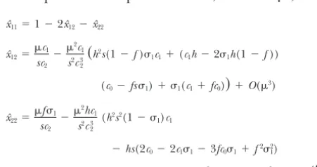
deter-xˆ11⫽1⫺2xˆ12⫺xˆ22 mines the sign ofFˆ_f⫽0(see Equations 2 and 3). When␫

is negative, the genotypes with the more extreme fitness xˆ12⫽ ␮

c1

sc2 ⫺ ␮2c1

s2_c3 2

共

h2_s(1⫺f)␴

1c1⫹(c1h⫺2␴1h(1⫺f))

(AA andaa) have a lower mean fitness on a log scale than the intermediate genotypes (Aa) and consequently (c0⫺fs␴1)⫹ ␴1(c1⫹fc0)

兲

become underrepresented within the population (Fˆf⫽0 becomes negative), with the reverse holding when␫is xˆ22⫽ ␮

f␴1

sc2 ⫺ ␮2hc1

s2_c3 2

(h2_s2₍₁⫺ ␴ 1)c1

positive.

⫺hs(2c0⫺2c1␴1⫺3fc0␴1⫹f2␴21) Selfing and other forms of inbreeding (f⬎0)

gener-ate a positive one-locus genetic association, ⫺ ␴1(c1⫹2fc0⫺sf2␴1))⫹O(␮3). (7)

Here and throughout this article,cidenotes a function, _Fˆ

f⬎0 ⫽f

␴1

1⫺(1⫺ ␴1)(1⫺s)

TABLE 2

Functions used to simplify the equations

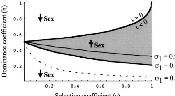
c0⫽1⫺(1⫺ ␴1)(1⫺s) c1⫽s(1⫺ ␴1)⫹ ␴1(1⫺f) c2⫽hc0⫹f␴1(1⫺h) c3⫽1⫺(1⫺ ␴2)(1⫺s) c4⫽1⫺(1⫺ ␴2)(1⫺hs) c5⫽1⫺(1⫺r␴2)(1⫺hs)

c6⫽r2(s⫹2␴2)2⫹4rs(␴2(1⫺2r␴2)⫹s(1⫺ ␴2)(1⫺r␴2)) c7⫽1⫺(1⫺ ␴3)(1⫺s)

c8⫽1⫺(1⫺ ␴3)(1⫺hs)

d0⫽(hs)2(␴2(1⫺2r␴2)⫹s(1⫺ ␴2)(1⫺r␴2))⫹(hs)r␴2(s⫹2␴2)⫺rs␴22

d1⫽(1⫺f)2␴1(␴3⫺ ␴2)

冢

冢

2⫺r

冣

⫹1

2c4(c7hs(hs⫹(1⫺hs)(2␴2⫺ ␴3))⫺c4c7d2⫺2(1⫺h)(1⫺s)hs␴ 2 3)

冣

⫺(1⫺f)sc4

冢

冢

2⫺r

冣

2(␴3⫺ ␴1)⫹h␴1(␴3⫺ ␴2)(c4c7⫹(1⫺h)s␴3)

⫹1

2␴2(␴3⫺ ␴1)(hs(2c4⫺d2⫺2(1⫺h)␴3)⫺c4d2)

冣

4hs2␴2(␴3⫺ ␴1)

d2⫽hs(1⫺ ␴3)⫹(2h⫺1)␴3 d3⫽1⫺2h⫺2hs⫹2h2s

For weak selection, the inbreeding coefficient given by 2r␴2

2r␴2⫹rs⫹

√

⬍ h⬍ 1

1⫹

√

(9) approachesf, as expected for a neutral locus under gametophytic selfing. Note that the one-locus genetic

The parameter range in which sex is favored shrinks as association will typically be orders of magnitude larger

selection becomes weaker, with both the left- and right-when generated by nonrandom mating (9) than right-when

hand side of (11) approaching1_⁄

2assgoes to zero. Sex generated by selection alone (8).

is favored over the broadest range of parameters when Stability analysis without inbreeding:To determine whether

deleterious mutations are lethal (s⫽1), in which case a modifier allele that alters an organism’s reproductive

modifiers that increase allocation to sexual reproduc-allocation (␴) to sexual vs. asexual reproduction will

tion spread for all dominance coefficients with tight invade or disappear when introduced at low frequency

linkage (r ⫽ 0) and for h ⬎ ␴2/(2 ⫹ ␴2) with loose within a population, I performed a local stability analysis

linkage (r⫽1_⁄

2). For lethal deleterious mutations (s⫽1), on the recursions (6) in the vicinity of the equilibrium

Equation 11 is equivalent to Equation A2.2a in Uyenoy-(7) (for a primer on stability analysis, see Appendices

ama and Bengtsson (1989). Although (11) appears in Bulmer1994 orRoughgarden1979). The fate of

not to depend on the current level of sex (␴1), the a rare modifier allele (m) depends on the eigenvalues

inequalities are easiest to satisfy when the modifier (␭) of the local stability matrix of (6). If all eigenvalues

causesMmheterozygotes to engage in a low frequency are less than one in magnitude, themallele declines in

of sex (small␴2), which requires that the initial popula-frequency over time. Conversely, if at least one

eigen-tion be primarily asexual for the modifier to increase the value is greater than one, allelemwill spread within the

frequency of sex (␴2⬎ ␴1). For dominance coefficients population. Without inbreeding (f⫽0), invasion of the

outside of the range given by (11), selection favors a modifier allele at a geometric rate is predicted to occur

decreased level of sex. These conditions are illustrated only when the following eigenvalue is greater than one:

in Figure 1. Considering the case of weak selection and partial recessivity of deleterious mutations as the most ␭f⫽0 ⫽1⫺ ␮2(␴2⫺ ␴1)

␫d0

h2_s2_c0c3c4c5⫹O(␮

3_{). (10)}

biologically relevant, these results indicate that modifi-ers that increase the frequency of sex would be selected In contrast to ci, the di denote functions (also defined against when inbreeding is absent. The strength of this

in Table 2) that are known to change sign depending selection is, however, extremely weak (O(␮2_)).

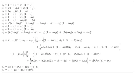
Figure 1.—Conditions under which a rare modifier that changes the frequency of sex with-out inbreeding (f⫽0) spreads within a popula-tion based on Equapopula-tion 10. Along the topmost curve, there are multiplicative fitness interactions within a locus (␫ ⫽ 0). For␴1 ⫽ 0.5, modifiers that increase the frequency of sex spread only in the shaded region, i.e., when ␫ is negative but weak. This region expands in less sexual popula-tions (␴1⫽0.1; dashed curve) and contracts in more sexual populations (␴1 ⫽ 0.9; thin solid curve). Other parameters are ␴2 ⫽ ␴1 ⫹ 0.01, r⫽1_⁄

2.

mine when evolution favors an increase in the frequency use to denote a modifier allele, m, that increases the frequency of sex (␴1ⱕ ␴2 ⱕ ␴3) or decreases it (␴1ⱖ of sexual reproduction given that sex involves selfing

or inbreeding (f ⬎0). The analysis indicates that a new ␴2ⱖ ␴3).

Equation 13 allows us to determine how the cutoff modifier allele spreads at a geometric rate only when

the following eigenvalue is greater than one: between regions in which sex is favored varies with

changing parameter values. For the following, I assume ␭f⬎0⫽1⫹ ␮

fd1

c2c4c8(␴2f⫹ ␴3(1⫺f))(c5c7(1⫺f)⫹c4sf)

that the modifier is directional and define␴2 ⫽ ␴1 ⫹ hM⌬␴and␴3⫽ ␴1⫹ ⌬␴, where⌬␴measures the homozy-gous effect of the modifier allele on the frequency of

⫹O(␮2_{). (12)}

sex andhM(0 ⱕ hM ⱕ 1) measures the dominance of

Invasion thus requires thatd1be positive. _{the modifier. From (13), it can be shown that}

Figures 2–4 illustrate the conditions under which a

i. d␪/dfⱕ 0. Higher rates of selfing/inbreeding de-modifier that increases the frequency of sex is able to

crease the cutoff, making it less likely that weakly spread. The evolution of sexual reproduction is favored

selected, partially recessive mutations favor sex (see in two regions. In region 1, selection is weak and

delete-Figure 3). rious mutations are recessive (bottom left-hand sides in

ii. d␪/d⌬␴ ⱖ0. Stronger modifiers increase the cutoff, Figures 2–4), and in region 2, selection is strong and

making it more likely that weakly selected, partially deleterious mutations are dominant (top right-hand

recessive mutations favor sex. sides in Figures 2–4).

iii. d␪/dhM ⬍ 0. More dominant modifiers decrease

In examining the figures, I noted that, for each

combi-the cutoff, making it less likely that weakly selected, nation of parameters, there was a value ofs, at which,

partially recessive mutations favor sex. In the spe-simultaneously, the curve delimiting region 1 crossed

cial case of a fully dominant modifier, the cutoff theh⫽0 axis and the curve delimiting region 2 crossed

goes to zero (Figure 2C). the h ⫽ 1 axis. At this exact point, called ␪, sex was

iv. d␪/d␴1 ⱖ 0. Higher rates of sex within the initial never favored, regardless of the dominance coefficient

population increase the cutoff, making it more (e.g., ␪ occurs at s ⫽ 0.31 in Figure 4). Because the

likely that weakly selected, partially recessive muta-leading eigenvalue equals one along these curves, I

de-tions favor sex (see Figure 2). termined the value of ␪ by setting h to either 0 or 1

v. d␪/dr ⫽ 0. The cutoff does not depend on the (the result was the same) in (12) and solving␭f⬎0 ⫽1

recombination rate. Although the cutoff does not fors, obtaining

change, it is possible to show that the region in which sex is favored to the left of the cutoff expands ␪ ⫽ (1⫺f)␴1␴3(␴3⫺ ␴2)

␴1␴3(␴3⫺ ␴2)⫹ ␴3(␴2⫺ ␴1)⫹f␴1(1⫺ ␴3)(␴3⫺ ␴2) .

in area for increasing recombination, while the re-(13) gion to the right of the cutoff decreases in area for increasing recombination (as seen in Figure 4). ␪, which marks the boundary between regions 1 and 2,

Thus, looser linkage makes it more likely that varies as a function of the frequency of sex (␴i, explored

weakly selected, partially recessive mutations favor in Figure 2) and the level of inbreeding (f, explored in

sex. Figure 3), but it is constant as a function of the rate of

recombination between the modifier and fitness loci (r, Next, let us consider the stability criterion for three explored in Figure 4). Note that the cutoff␪lies between cases of special interest. First, when selection is weak,

Figure2.—Conditions under which a modifier that changes the frequency of sex spreads within an inbreeding population. In A, the modifier is recessive (␴2 ⫽ ␴1; ␴3 ⫽ ␴1 ⫹ 0.01); in B, the modifier is additive (␴2⫽ ␴1⫹0.005;␴3⫽ ␴1⫹ 0.01); in C, the modifier is dominant (␴2⫽ ␴1⫹ 0.01;␴3⫽ ␴2). When sexual and asexual reproduc-tion are equally frequent (␴1 ⫽ 0.5), increased sex is favored within the shaded areas. Typically, there are two regions in which a modifier that increases the frequency of sex spreads: (1) Delete-rious mutations are weakly selected and partially recessive and (2) deleterious mutations are strongly selected and partially dominant. The boundary between the two regions (␪) is indicated on thex-axis for␴1⫽0.5. These regions shift to the left in less sexual populations (␴1 ⫽ 0.1; dashed curves) and shift to the right in more sexual populations (␴1⫽0.9; thin solid curves). Increasing the modifier’s level of dominance con-tracts the first region and expands the second region, to the point that the first region entirely disappears when the modifier is completely domi-nant (C). Other parameters aref⫽0.05,r⫽0.5.

␭sⰆ1⫽1⫹ ␮

f(1⫺f) (1⫺2h)(␴3⫺ ␴2)

(f⫹(1⫺f)h)(f␴2⫹(1⫺f)␴3)

⫹O(␮s,␮2_{). (14)}

⫹O(␮(1⫺f),␮2_{). (15)}

Thus, a rare modifier allele that causes more sex (␴3⫺ Thus, for weak selection, a modifier allele that increases

␴1 ⬎ 0) is always able to invade if inbreeding is high allocation to sexual reproduction spreads whenever

del-enough among the individuals that reproduce sexually eterious mutations are partially recessive (0ⱕh⬍1_⁄

2), as

(barring h ⫽ 0). Third, if the modifier introduces a long as the rare modifier is not fully dominant. Second,

small amount of sex (⌬␴ Ⰶ1) into a fully asexual popula-when sexual reproduction involves high levels of selfing

tion, the governing eigenvalue becomes (fnear 1), the governing eigenvalue becomes

␭␴1⫽0⫽1⫹ ␮

f␴2␴3 hs(f␴2⫹(1⫺f)␴3)

⫹O(␮2_,⌬␴2_{). (16)} ␭fⵑ1⫽1⫹ ␮

hs(␴3⫺ ␴1)

Figure3.—The effect of the inbreeding rate on the conditions under which a mod-ifier of sex spreads. The two regions in which sex is favored are shaded for interme-diate inbreeding levels (f⫽0.1), with their boundary occurring at ␪. These regions shift to the right in less inbred populations (f⫽0.0001; dashed curves) and shift to the left in more inbred populations (f⫽ 0.5; thin solid curves). The regions in which sex is favored depend only weakly onf, unless inbreeding is common. While the curves are drawn using Equation 12, which as-sumes that fⰇ ␮, nearly identical curves are generated by exact numerical calcula-tions of the eigenvalues with ␮ ⫽ 10⫺6_. Other parameters are␴1⫽0.5,␴2⫽ ␴1⫹ 0.005,␴3⫽ ␴1⫹0.01, andr⫽0.5.

Thus, a weak modifier allele is always able to invade an Simulation check: Deterministic simulations of the re-cursions were run using Mathematica 3.0 (Wolfram asexual population (barringh ⫽ 0). Strong modifiers

that cause a substantial amount of sex within an other- 1991) to confirm that the above stability analyses cor-rectly identified the conditions under which sex is fa-wise asexual population spread, however, only if

domi-nance (h) is sufficiently high. vored. The parameters chosen were identical to those

in Figures 1 and 2, withhandsset to every combination Although the above analysis assumes gametophytic

selfing,Uyenoyama andBengtsson (1989) obtained of {0.01, 0.1, 0.2, 0.3, . . . , 0.8, 0.9, 1.0} and with ␮ ⫽ 10⫺6_{. The frequencies ofAA,Aa, andaagenotypes were} similar results assuming sporophytic selfing and lethal

mutations (s⫽ 1). In the absence of selection, sporo- set to the mutation-selection balance described by (7). The frequencies ofMM,Mm, andmmgenotypes were set phytic selfing at rateb generates an inbreeding

coeffi-cient ofF ⫽ b/(2 ⫺ b) (Uyenoyama and Bengtsson top2

M(1⫺ f)⫹fpM, 2pMpm(1⫺ f), and p2m(1⫺ f)⫹fpm,

respectively, with the frequency of allelem(pm⫽1⫺pM)

1989), while gametophytic selfing at ratefresults inF⫽f.

Thus, to compare the two forms of selfing, I setf⫽b/ set to 0.001 and the selfing rate (f) set to 0 (for Figure 1) or 0.05 (for Figure 2). Linkage disequilibrium be-(2 ⫺ b). Both Equation 12 and their results indicate

that, whens ⫽1, sex is favored as long as his greater tween theM and A loci was initially set to zero. The simulations were run for 10,000 generations withf⫽0 than a threshold value (see right-hand edge of Figures

2–4). This threshold value differs quantitatively but not and for 1000 generations with f ⫽ 0.05, and the total change in the modifier frequency was scored. For every qualitatively between the two analyses.

In contrast to the case where inbreeding was absent, parameter combination examined except four cases where no appreciable change in modifier frequency these results indicate that modifiers that increase the

frequency of sex are positively selected when inbreeding occurred (all near the curves withF⫽0), the modifier rose in frequency when predicted by the regions de-is present for the most biologically relevant case of weak

selection and partial recessivity of deleterious muta- limited in Figures 1 and 2.

Evolutionary stable strategy: We turn now to the long-tions, as long as a rare modifier is not fully dominant.

Figure4.—The effect of recombination on the

conditions under which a modifier of sex spreads within an inbreeding population. The two regions in which sex is favored are shaded for an interme-diate recombination rate between the modifier and selected loci (r⫽ 0.1). Region 1 contracts and region 2 expands when the loci are more tightly linked (r⫽0.01; dashed curves), and the converse is observed for looser linkage (r⫽0.5; thin solid curves). Other parameters are␴1⫽0.5,

term evolution of the system and ask whether there is a level of sex at which the population will remain and be stable to invasion by any new allele that arises and modifies the frequency of sex. This level of sex repre-sents an evolutionary stable strategy (ESS; Maynard Smith1982). Because the strength of selection acting on the modifier is negligibly weak in the absence of inbreeding, we focus only on the case with inbreeding (analysis without inbreeding is available upon request). When inbreeding is present, we must determine whether a value of␴1exists (␴*1) that cannot be invaded by any modifier allele causing the frequency of sex to change to ␴2 in heterozygotes and␴3 in homozygotes from the eigenvalue (12). Let us begin with the border solutions (␴*1 ⫽ 0 or 1). From (16), an asexual popula-tion (␴*1 ⫽0) can be invaded by modifiers that intro-duce sex at sufficiently low rates. Thus, a fully asexual population is never an ESS. A population that is fully sexual (␴*1 ⫽ 1) is stable to invasion by any weak mod-ifier allele when inbreeding is common, specifically, when

f⬎[d3hs⫹r(1⫺hs)(2d3⫺(1⫺2h)s)

⫹s√h2_{⫺2hr(1⫺hs)(d}

3⫺2(1⫺h)2s)⫹r2(1⫺2h)2(1⫺hs)2]/[2d3r(1⫺hs) ⫹2hs(1⫺h)(1⫺hs⫹s)] ,

(17)

as illustrated in Figure 5. Numerical analyses suggest that, if the above condition holds and weak modifiers are unable to invade, then strong modifiers (␴2,␴3Ⰶ1) are also unable to invade.

Interestingly, full sexuality (␴*1 ⫽1) is the only ESS with alleleMfixed of this model with inbreeding. Any intermediate value of␴*1 can always be invaded by some weak modifier if we allow all possible levels of domi-nance for the modifier. This can be shown by noting that an intermediate ESS must satisfy both

Figure 5.—The ESS level of sex with inbreeding. For a

given level of inbreeding (f), complete sexuality (␴*1 ⫽1) is d␭f⬎0

d␴2

冨

⫽0 and d␭f⬎0 d␴3

冨

␴3⫽␴*1

⫽0 ,

an ESS when selection is sufficiently strong (to the right of the contours; Equation 17). For example, withf⫽1, complete sexuality is an ESS over the entire parameter range, while, whenf⫽0.1, it is an ESS only in the last region at the top right of the graph. To the left of the contours there is no ESS,

but these describe two different equations in one un-known (␴*1) that cannot be satisfied simultaneously.

as there are always some combinations of␴2and␴3that allow That this might be true can be gleaned from Figure 2. _{a modifier to invade. A shows the case with free recombination} Consider the case wheref⫽0.05,␴1⫽0.9,r⫽1⁄2,s⫽ between the modifier and fitness locus (r⫽1_⁄

2); B shows the 0.4, and h⫽ 0.097. This case falls on the solid line in case with complete linkage (r⫽0).

Figure 2B, indicating that a weak additive modifier that increases or decreases sex cannot invade. Figure 2A

indicates, however, that a weak recessive modifier that populations with both sexual and asexual reproduction. Instead, we predict that the level of sexuality should increases the frequency of sex could invade, and Figure

2C indicates that a weak dominant modifier that de- fluctuate up and down over evolutionary time,

de-pending on the exact sequence of modifier alleles that creases the frequency of sex could invade. Given that

there is no reason to believe that modifier alleles that appear within the population. Nevertheless, the long-term average level of sexuality will depend on the selec-alter the allocation to sexual and asexual reproduction

be more common over evolutionary time when domi- _⌽f⬎

0;sⰆ1⫽

兺

i⫽1

(␭f⬎0⫺1) nance (h) and selection coefficients (s) are both low or

both high.

⫽U(␴3⫺ ␴2)

f(1⫺f)(1⫺2h) 2(f⫹(1⫺f)h)(f␴2⫹(1⫺f)␴3) Genome-wide strength of selection: Here I estimate the

genome-wide strength of selection acting on a modifier

⫹O(sU,␮U). (19a)

of sex assuming free recombination between all loci. Con-siderLfitness loci scattered throughout the genome, with

As long as the modifier is not completely dominant and no linkage disequilibrium between them, as might be

as long as deleterious mutations are partially recessive expected if the fitness effects of each locus are

indepen-(0ⱕh⬍ 1_⁄

2), weak selection against deleterious

muta-dent and multiply together (Maynard Smith 1968;

tions favors the evolution of sex with a force that is propor-Eshel and Feldman 1970). The strength of indirect

tional to the genome-wide mutation rate times the effect selection acting on a modifier allele through its effects _{of the modifier (␴}

3⫺ ␴2) times the inbreeding coeffi-on segregaticoeffi-on at any coeffi-one locus may be defined asφ⬅

cient. The above calculations fail, however, to take into ␭ ⫺1, where␭is the leading eigenvalue. It can be shown

account the wide variation in dominance and selection that, if the modifier allele is rare and selection is weak,

coefficients among mutations. To make accurate predic-φ measures the asymptotic rate at which a modifier

tions regarding the effects of segregation on the evolu-changes in frequency:

tion of sex requires us to integrate over the joint distribu-tion ofhands. Although this distribution is unknown, φ⬇ p⬘m⫺pm

pMpm

. _{data from Drosophila suggest that a small percentage}

of deleterious mutations (ⵑ5%) are lethal, and these Under the above assumptions, each fitness locus has only tend to be more highly recessive (hⵑ 0.02–0.03) than a small and independent effect on the frequency of the mildly deleterious mutations (SimmonsandCrow1977;

modifier, so we may sum the φ over the number of CharlesworthandCharlesworth1999). Thus, it is

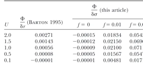
fitness loci (L) to get the genome-wide indirect effect worth asking whether the impact of relatively rare, lethal mutations outweighs the impact of mildly deleterious of selection on a modifier of sex (⌽).

mutations on the evolution of sex. The genome-wide In the absence of inbreeding, the genome-wide

indi-selective force on a modifier arising from such lethals rect selection on a rare modifier is

can be simplified by assuming a weak additive modifier

⌽f⫽0⫽

兺

L

i⫽1

⫺ ␮2_(␴

2⫺ ␴1) in Equation 12, yielding

⌽f⬎0;s⫽1⫽ ⫺Ulethal(␴2⫺ ␴1) ⫻ (1⫺2h⫹h2s)(␴2(1⫺2h⫹hs)⫺2hs)

h2_(s⫹ ␴

1(1⫺s))(s⫹ ␴2(1⫺s))(2hs⫹ ␴2(1⫺hs))

⫻ f((1⫺f)(1⫺h)␴1 ⫺h(1 ⫹f)) 2(h⫹ (1⫺h)␴1)(h⫹ (1⫺h)f␴1)

⫹O(␮3_{) (18a)}

⫹ O(⌬␴2_Ulethal,␮_{lethalUlethal). (19b)} (from Equation 10). For each locus, the values ofh,s,

and␮will differ. Thus, this sum depends on the joint _{Except in populations with very little sex (␴}

1 small), distribution of these parameters, which is unknown. As- _{lethal mutations that are highly recessive tend to select} suming, for the sake of argument, that there is little _{against sex, but given that lethals account for only a} variance in each parameter and that selection is weak, _{fraction of deleterious mutations, (19b) tends to} repre-the total strength of indirect selection on repre-the modifier _{sent a smaller selective force than (19a) does. For}

exam-becomes _{ple, if␴}

1⫽0.5,f⫽0.05,h⫽0.1 for weakly deleterious mutations, h ⫽ 0.02 for lethal deleterious mutations, ⌽f⫽0⬇⫺␮U(␴2⫺ ␴1)

(1⫺2h)2 2h2_␴

1␴2

⫹O(␮sU,␮2_U),

andUlethalis 5% of the total deleterious mutation rate, the strength of selection acting on a modifier arising (18b)

from lethal mutations is only 10% of that arising from weakly deleterious mutations. Thus the combined force whereU is the mutation rate per diploid genome per

generation (U⫽ 2L␮) and a bar over a parameter de- of many mild deleterious mutations and few lethal muta-tions still tends to favor the evolution of sex.

notes its average value. This genome-wide force selects

against sex but is exceedingly weak (proportional to The above discussion assumes that sex entails no di-rect fitness costs (e.g., costs associated with searching the per-locus mutation rate) unless mutations are very

nearly recessive, such that the denominator in (18a) is for and courting mates, producing males, etc.). We can incorporate such fitness costs, ␦, by multiplying the on the order of␮.

Much stronger selection on the modifier is observed terms in Equations 6 representing sexual reproduction by (1⫺ ␦) and renormalizing. To simplify the analysis, when inbreeding is present. For weak selection (sⰆ1;

tions. Modifier alleles now change in frequency in re- tion (22) harder to satisfy. This is because the cost of sex reduces the effective level of genetic mixing within sponse to two forces: the direct costs of sex (measured

by ⌿) and the indirect effects of altering segregation a population, causing the initial population to be similar to a more asexual population in which the advantages patterns at selected loci (measured byφper locus and

⌽per genome). Only if the net effect is positive (⌿ ⫹ of sex are greater. The above assumes, however, that the modifier is weak, so that the modifier alleles differ ⌽ ⬎0) will a modifier allele spread. To determine⌿,

the local stability analysis was performed by fixing the very little in the cost of sex imposed upon them; numeri-cal examples suggest that the costs of sex are less likely Aallele at the selected locus (i.e., by setting␮ ⫽0) and

by defining ⌿⬅␭ ⫺1, yielding to be counterbalanced by the benefits of segregation

for modifier alleles that cause large increases in the frequency of sex. The above also assumes that selection ⌿ ⫽ ⫺ ␦((1⫺f)(␴2⫺ ␴1)⫹f(␴3⫺ ␴1))

1⫺ ␦␴1

, (20)

at the fitness loci (s) is weak. With stronger selection, both the intrinsic costs of sex and the effects of sex on which is negative for a modifier that increases the

fre-segregation can select against modifiers that increase quency of sex. Equation 20 equals the difference

be-the frequency of sex (see Figures 2–4). Neverbe-theless, tween the cost of sex paid by the old and new modifier

this analysis indicates that the inclusion of substantial alleles and is small whenever the modifier only slightly

costs of sex is not fatal to the hypothesis that the conse-alters the frequency of sex. Next, mutations were

rein-quences of segregation might have shaped the evolution corporated into the model, and a stability analysis was

and maintenance of sex. performed near the mutation-selection equilibrium.

Directional selection:Quasi-linkage equilibrium (QLE):

The indirect effect of the modifier per locus was defined

Segregation could also provide an advantage to sex when asφ ⬅ ␭ ⫺ 1⫺ ⌿, which was summed across loci to

populations are adapting to new environments. Insight get the net indirect effect of the modifier, ⌽, again

into the dynamics of nonequilibrium populations can be ignoring variation in the parameters. In the absence of

gained using a method introduced byKimura(1965), inbreeding (f⫽0), ⌽is only on the order of the

per-known as a quasi-linkage equilibrium (QLE) analysis locus mutation rate and hence is negligible relative to

(seeBartonandTurelli1991). The critical assump-the costs of sex. With inbreeding, however, assump-the indirect

tion made in a QLE analysis is that genetic associations selective force on a modifier is

reach an approximate balance between the forces that generate associations (e.g., selection, drift, and inbreed-⌽␦⬎0;sⰆ1⫽U

1⫹ ␦

1⫺ ␦(␴3⫺ ␴2)

f(1⫺ f)(1⫺2h)

2(f⫹ (1⫺f)h)␴1 ing) and those that break them down (e.g., sex and recombination) as long as the forces breaking down ⫹O(sU,⌬␴2_U, ␮_{U), (21)}

associations are sufficiently strong. Under this condi-tion, genetic associations rapidly reach quasi-equilib-which differs slightly from (19a) because of the

assump-rium at every point along the allele frequency trajectory. tion of a weak modifier (reflected in the␴1term) and

To solve for the QLE level of association, one sets the because the cost of sex reduces the efficacy of sexual

change in each association to zero and solves for its reproduction in breaking down genetic associations

[re-quasi-equilibrium value as a function of the current flected in the (1⫹ ␦)/(1⫺ ␦) term]. Overall, the effects

allele frequencies. Throughout the following I use the of a modifier on segregation will overwhelm the costs of

central-moment association measures as defined in Bar-sex only if the sum of (20) and (21) is positive. For a

tonandTurelli(1991) andKirkpatricket al.(2002). modifier that increases the frequency of sex, this requires

These describe the gametic-phase linkage disequilib-that mutations be partially recessive (0ⱕh⬍1_⁄

2) and

rium (D ⫽ y1y4 ⫺ y2y3), the linkage disequilibrium be-U⬎2␴1␦(1⫺ ␦)((1⫺f)(␴2⫺ ␴1)⫹f(␴3⫺ ␴1))(f⫹(1⫺f)h)

(1⫺ ␦␴1)(1⫹ ␦)(␴3⫺ ␴2)f(1⫺f)(1⫺2h). tween alleles on homologous chromosomes, the

depar-ture from Hardy-Weinberg at locus A(the numerator (22)

ofFin Equation 1), the departure from Hardy-Weinberg at locus M, the association between a modifier allele Condition (22) indicates that a modifier that causes a

slight increase in the frequency of sex can invade despite and the departure from Hardy-Weinberg at the viability locus, the association between a viability allele and the a twofold cost of sex (␦ ⫽1_⁄

2) as long as the

genome-wide deleterious mutation rate (U) is high enough and/ departure from Hardy-Weinberg at the modifier locus, and the association between the departure from Hardy-or the frequency of sex (␴1) is initially low enough. As

an example, when f ⫽ 0.05 and h ⫽ 0.1, the current Weinberg at the modifier locus and the departure from Hardy-Weinberg at the viability locus. These seven asso-allocation to sexual reproduction must be ⬍ⵑ54% if

U⫽1 or 7% ifU⫽0.1 for sex to evolve. These calcula- ciation measures, along with the frequencies of the A and m alleles (pA and pm, respectively), provide nine

tions indicate that the advantages of segregation can be

strong enough within inbreeding populations to select independent equations that completely describe the dy-namics and can be used to replace the genotypic fre-for costly sex, especially when sex is currently rare.

QLE without inbreeding: To find the QLE without in- (pA,0near 0) to a high final frequency (pA,Tnear 1), the

above simplifies to breeding (f⫽0), it was assumed that selection is weak

[s ⫽ O(␰)] and that the modifier is weak [␴2 ⫽ ␴1 ⫹

⌬pm,total⬇⫺spMpm⳵␴

␴2 1

冦

1 2⫺

h(1⫺h) (1⫺2h)Log

冤

1⫺h

h

冥冧

O(␰) and ␴3 ⫽ ␴1 ⫹O(␰)], where␰is some small term (␰ Ⰶ1). The QLE values for each association measure were solved, keeping terms up toO(␰2_{), and then used}

The factor in braces is nearly quadratic in shape and to determine the change in frequency of the modifier falls from1_⁄

2ath⫽0 to 0 ath⫽1⁄2and then rises back allele (⌬pm⫽ p⬘m⫺pm). The resulting equation for the to1⁄₂ath ⫽ 1. Thus, the total strength of selection on

per-generation change in the modifier is the modifier (sm,total⫽ ⌬pm,total/(pMpm)) arising per

selec-tive sweep is⬍ ⫺⳵␴s/(2␴2

1) when inbreeding is absent. ⌬pm⫽ ⫺s2pMpm

⳵␴ ␴2 1

(1 ⫺2h)2_(p

Apa)2⫹O(␰4), (23) Consequently, the total amount of selection acting on

the modifier locusMamounts to less than one genera-tion’s worth of selection on locusA, unless sex is rare. where

Note, however, that the QLE approximation will break ⳵␴ ⫽(␴2⫺ ␴1)pM ⫹ (␴3⫺ ␴2)(1⫺pM). _{down if sex is so rare that selection builds genetic}

associ-ations faster than sex breaks them down. (The derivation of Equation 23 assumes that h is not

QLE with inbreeding: A similar QLE analysis was con-very near 1_⁄

2. For nearly additive beneficial alleles, see

ducted assuming that sexual reproduction occurs with Equation 31.) Equation 23 indicates that, under weak

inbreeding. The following equations for the change in selection, modifiers that increase the frequency of sex

the frequency of the modifier must be added to the are always selected against. To leading order ins,

Equa-above QLE results without inbreeding. Unless inbreed-tion 23 is identical to the per-generainbreed-tion change in the

ing levels are low [O(␰) or smaller], however, inbreeding modifier expected at mutation-selection balance (1⫺

causes a greater change in the modifier and so the ␭f⫽0from Equation 10) under the combined set of

as-previous terms may be neglected. Per generation, the sumptions: The modifier is weak, mis rare, and pA is

modifier allele changes in frequency by near the equilibrium described by Equation 7. Thus,

under directional selection as well as at a

mutation-⌬pm⫽ spMpm

ⵜ␴ ␴1

(1 ⫺2h)f(1⫺f)pApa⫹O(␰3), (27)

selection balance, weak selection on locusAgenerates indirect selection against a modifier allele that increases

where allocation to sexual reproduction as long as inbreeding

is absent.

ⵜ␴ ⫽(␴2⫺ ␴1)(1⫺ pM)⫹(␴3⫺ ␴2)pM.

How strong is this force? As the Aallele rises in

fre-quency frompA,0at time 0 topA,Tat timeT, the cumulative For this QLE approximation to be valid, sex must be

change in the modifier allele would be _{frequent relative to the rate of inbreeding (␴1 Ⰷ f);}

otherwise the genetic associations are slow to reach ⌬pm,total⬇

冮

T

t⫽0 ⫺s2_p

Mpm

⳵␴ ␴2 1

(1⫺2h)2_(p

Apa)2dt. (24) steady state. Equation 27 indicates that a directional

modifier allele that increases the frequency of sex will spread whenever h ⬍ 1_⁄

2 under weak selection. Again, Under the assumptions of weak selection and frequent

to leading order ins, Equation 27 is identical to the per sexual reproduction, we may approximate the

per-gen-generation change in the modifier expected at muta-eration change inpAby the differential equation

tion-selection balance (1⫺ ␭f⬎0from Equation 12) un-der the combined set of assumptions. There is, however, dpA

dt ⬇ p⬘A⫺pA ⬇spApag(pA), (25) a key biological difference: The requirement thathbe ⬍1_⁄

2implies that deleterious mutations must be partially where

recessivebut beneficial mutations must be partially domi-nantfor sex to be favored.

g(pA)⫽ (1⫺h)(1⫺ pA)⫹hpA.

Equation 27 may be integrated over a selective sweep Transforming the independent variable in Equation 24 _{using Equation 25 to rewrite time in terms of the allele} from time (t) to allele frequency (pA), using Equation _frequency,p

A, where nowg(pA)⫽(1⫺f)((1⫺h)(1⫺

25 and integrating, we get _p

A)⫹ hpA)⫹ f. The total change in the modifier per

generation is then ⌬pm,total⬇⫺spMpm⳵␴

␴2 1

⌬pm,total⬇ pMpm

ⵜ␴ ␴1

fLog

冤

冥

. (28)

⫻

冢

2 ⫺

h(1⫺h) (1⫺2h)Log

冤

g(pA,0) g(pA,T)

冥

冣

.

For a directional modifier that increases the frequency (26a)

of sex, Equation 28 is positive ath ⫽ 0, declines with increasingh, reaches 0 ath⫽1_⁄

Figure6.—The total change in frequency of a modifier allele that increases allocation to sexual reproduction over the course of a selective sweep. The plots scale the total change as ⌬pm,total/ (pMpm␦␴), which represents the selection gradient acting on the modifier, assuming a weak additive modifier (␴3⫽ ␴1⫹2␦␴). A is without inbreeding (f⫽0; using Equation 26a); B is with inbreeding (f⫽ 0.05; using the sum of Equations 26a and 28). The long dashed curves are the analytical results and the circles are the simulation results when sexual and asexual reproduction are equally frequent (␴1⫽0.5). The solid curves are the ana-lytical results, and the squares are the simulation results when sex is initially common (␴1⫽0.9). Other parameters are␴2⫽ ␴1⫹0.005,␴3⫽ ␴1⫹ 0.01,r⫽0.5,pA,0⫽0.001,pA,T⫽0.999,pM,0⫽0.999, ands⫽0.01. As selection becomes stronger, the analytical results become less accurate.

forh ⬎1_⁄

2. In the case where the beneficial allele rises served in simulations. Further simulations (available upon request) demonstrate, however, that the QLE pre-from a low initial frequency (pA,0near 0) to a high final

frequency (pA,Tnear 1), (28) becomes approximately dictions can be off by as much as a factor of five if either sor␴1 is set to 0.1.

As noted after Equations 23 and 27, the QLE results ⌬pm,total⬇2pMpmⵜ␴

␴1

f(1 ⫺f)

1⫹f (1⫺ 2h), (29) _{with directional selection are equivalent to those} ob-tained at a mutation-selection balance when selection where the approximation works best near h ⫽ 1_⁄

2 and

is assumed to be weak. Simulations were performed underestimates the change in the modifier for h near

to explore whether the results remain similar under zero or one. Equations 28 and 29 indicate that each

stronger selection. Without inbreeding, simulations in-selective sweep within a genome causes a modifier allele

dicate that the answer is “yes” (Figure 7A). With inbreed-that promotes sexual reproduction to rise in frequency,

ing, however, the conditions that favor sex at mutation-as long mutation-as beneficial alleles are weakly selected and

par-selection balance and under directional par-selection differ, tially dominant. Now the total amount of selection

act-especially as selection becomes stronger (Figure 7B). ing on the modifier depends not onsbut onfand will

The discrepancy diminishes when the simulations are be substantial when inbreeding rates are high.

allowed to run for longer while the a allele is rare, as Simulation check: The above QLE predictions were

is the case at mutation-selection balance. Nevertheless, compared to deterministic simulations, which were

per-the qualitative result remains that sex, with inbreeding, formed as described for the case of a mutation-selection

is favored when dominance levels are low and selection balance with the following exceptions. The A allele

is weak or when dominance levels are high and selection started at a frequency of 0.001, and the simulations were

is strong. run until A reached a frequency of 0.999. Mutations

were ignored. The initial frequencies ofAA,Aa, andaa genotypes were set to p2

A(1⫺f)⫹fpA, 2pApa(1⫺ f),

COMPARISONS TO OTHER MODELS AND

andp2

a(1⫺f)⫹fpa, respectively. Finally, weak selection

INTERPRETATION

(s⫽0.01) and high initial frequencies of sex (␴1⫽0.5

or 0.9) were assumed, as required for the QLE analysis The results derived above demonstrate that selection acts on a modifier of sex in complex ways. Some intuitive to be valid. Figure 6 illustrates that the QLE analysis