Comparing Analysis Methods for Mutation-Accumulation Data:
A Simulation Study
Aurora Garcı´a-Dorado
1and Araceli Gallego
Departamento de Gene´tica, Facultad de Biologı´a, Universidad Complutense de Madrid, 28040 Madrid, Spain Manuscript received December 29, 2002
Accepted for publication March 11, 2003
ABSTRACT
We simulated single-generation data for a fitness trait in mutation-accumulation (MA) experiments, and we compared three methods of analysis. Bateman-Mukai (BM) and maximum likelihood (ML) need information on both the MA lines and control lines, while minimum distance (MD) can be applied with or without the control. Both MD and ML assume gamma-distributed mutational effects. ML estimates of the rate of deleterious mutation had larger mean square error (MSE) than MD or BM had due to large outliers. MD estimates obtained by ignoring the mean decline observed from comparison to a control are often better than those obtained using that information. When effects are simulated using the gamma distribution, reducing the precision with which the trait is assayed increases the probability of obtaining no ML or MD estimates but causes no appreciable increase of the MSE. When the residual errors for the means of the simulated lines are sampled from the empirical distribution in a MA experiment, instead of from a normal one, the MSEs of BM, ML, and MD are practically unaffected. When the simulated gamma distribution accounts for a high rate of mild deleterious mutation, BM detects onlyⵑ30% of the true deleterious mutation rate, while MD or ML detects substantially larger fractions. To test the robustness of the methods, we also added a high rate of common contaminant mutations with constant mild deleterious effect to a low rate of mutations with gamma-distributed deleterious effects and moderate average. In that case, BM detects roughly the same fraction as before, regardless of the precision of the assay, while ML fails to provide estimates. However, MD estimates are obtained by ignoring the control information, detectingⵑ70% of the total mutation rate when the mean of the lines is assayed with good precision, but only 15% for low-precision assays. Contaminant mutations with only tiny deleterious effects could not be detected with acceptable accuracy by any of the above methods.
T
HE properties of mutations affecting fitness and its The Bateman-Mukai (BM) procedure, which has the component traits are relevant to many evolutionary advantage of simplicity, is more frequently used (see and conservation issues, and an important experimental Mukaiet al. 1972). It estimates a lower bound for the effort is currently being devoted to their understanding. rate of mutation affecting a fitness trait per gamete and A widely used procedure is the mutation-accumulation generation () and an upper bound for the correspond-(MA) design where, by relaxing natural selection as ing expected deleterious effect,E(s), using the trait’s much as possible, deleterious mutations are allowed to rates of increase in variance (⌬V) and decline in mean accumulate in replicate lines derived from a common, (⌬M) caused by mutation. The validity of these bounds genetically invariable, origin. This procedure provides is quite general, but their closeness to the true and information on both the rate and the effect of muta- E(s) values (and, therefore, their usefulness) decays as tions, which do not rely on the assumption of mutation- the variance of the deleterious effect increases. selection balance (see reviews byGarcı´a-Doradoet al. The second approach is a maximum-likelihood (ML) 1999;KeightleyandEyre-Walker 1999; andLynch one, requiring some assumptions on the distribution et al.1999; and recent experiments byVassilievaet al. of the deleterious effects (s). This method has been 2000; Chavarri´as et al. 2001 and Shaw et al. 2002. implemented byKeightley(1994), assuming a gamma-However, these inferences are indirect and require the distributed s or a constant deleterious effect (S). It use of statistical techniques whose properties depend searches for the mutation rate and the gamma parame-on many factors, such as the shape of the distributiparame-on ters (or theSvalue), maximizing the likelihood of the of mutational effects and the magnitude of the residual observed distribution of the means of the MA and con-errors. Basically, the following three methods have been trol lines. Here we concentrate on the more widely used used to analyze MA data. gamma alternative. The method has been extended to a reflected gamma distribution, where|s|is gamma dis-tributed buts has negative sign with some probability1Corresponding author:Departamento de Gene´tica, Facultad de
Bio-(Keightleyand Ohnishi1998). Under the more
re-logı´a, Universidad Complutense de Madrid, 28040 Madrid, Spain.
E-mail: [email protected] strictive assumption of constant deleterious effects, the
method has been further extended to analyze multigen- lines and control are assayed only once at the end of the MA period. The properties of the MD method are eration data (KeightleyandBataillon2000).
analyzed both using and not using the information pro-The third method is minimum distance (MD), and
vided by the control. To simulate the data, we use nor-it also requires the assumption of a distribution fors.
mally or nonnormally distributed sampling errors. To It has been implemented by Garcı´a-Dorado by assuming
check the robustness of the different estimation meth-either a reflected gamma or a mixed normal-gamma
ods against departures from the model assumed, we distribution fors(seeGarcı´a-Dorado1997). Here we
introduce mutations with small constant deleterious ef-concentrate on the reflected-gamma alternative. This
fects, not fitting within the gamma distribution. method searches for the mutational parameters (i.e.,
the mutation rate and the parameters of the reflected gamma) that minimize the Cramer-von Mises distance
MATERIALS AND METHODS between the observed and theoretically predicted
distri-bution of the line means, as is explained in the next The background accumulation model section.
For convenience, we consider a fitness trait that we denote MD results have generally been obtained conditional
viability and a set of isolated MA lines derived from a common on an estimate of⌬Vbut not necessarily on one of⌬M. isogenic strain. We assume that the number of deleterious This is of particular interest since this⌬Mis estimated mutations occurring per gamete and per generation is Poisson distributed with mean, so that 2Nnew single-copy deleteri-by comparison to a control population, and maintaining
ous mutations are expected to occur per generation in theN a reliable control (efficiently protected against both the
breeding individuals of each MA line. We consider nonsevere accumulation of deleterious mutations and the selection deleterious mutations that randomly drift in the MA lines due of advantageous ones) is loaded with pitfalls. ForFer- to their very low population size, so that any new mutation has
a final fixation probability 1/(2N). Therefore, MA individuals
na´ndezandLo´ pez-Fanjul(1996) Drosophila MA data,
sampled at generationtare expected to be homozygous for MD estimates characterized by low mutation rates and
Fxtmutations that occurred at generationx, whereFxtis the moderate average deleterious effects have been ob- probability of identity by descent at generation
t taking x tained regardless of whether or not the control informa- as the reference noninbred generation. Thus, considering tion is used. These MD estimates were similar to the mutations that occurred at all previous generations, MA
indi-viduals are expected to be homozygous forU⫽ Fc
tnew muta-corresponding BM ones (Garcı´a-Doradoet al.1998).
tions, whereFc
t ⫽兺x⬍tFxtis the “forward cumulated inbreed-Low rates and moderate effects were also obtained from
ing coefficient.” Since each mutation is assumed to be unique, MD analysis of Mukai’s classical MA data (Mukaiet al. individuals from different MA lines will be homozygous for 1972) if the large ⌬M observed was ignored. In that different mutations. Thus, the number of mutations accumu-lated per MA line at generationtis Poisson distributed with analysis, the MD estimate ofwas one order of
magni-meanU. The between-line genetic variance and overall viabil-tude lower than that of the BM, suggesting that the
ity mean at generationtare, respectively, large ⌬M observed by Mukai et al. (1972) could be
biased (Garcı´a-Dorado et al. 1998). However, it has 2
G⫽FctE(s2)⫽UE(s2), been argued that the MD method is unable to detect
t⫽ 0⫺FctE(s)⫽ 0⫺UE(s), mildly deleterious mutation and is strongly biased due
where0is the mean viability of the original isogenic strain, to sampling errors departing slightly from normality
before mutation accumulation. In general,Fc
t/tasymptotically
(Lynchet al.1999). approaches 1 for increasingt. In those experiments where a
Since MA experiments are extremely time- and work- single copy of the MA genome or chromosome is transferred consuming, it is of obvious practical interest to study per generation and line,Fc
tequals the numbertof MA genera-tions. Thus, in the following, we usetinstead ofFc
t for sim-the properties of sim-the above statistical techniques to
plicity. choose, in each case, the one extracting maximum
infor-mation from the data. For this purpose, several
simula-Simulating data tion studies have been carried out (Garcı´a-Dorado
1997;Keightley1998;Denget al. 1999). However, the To investigate the different estimation methods, we simu-relative merits of the different methods have not been lated sets of diploid lines that were evaluated once for viability, established. Furthermore, in the ML and MD studies after a given MA period during which deleterious mutations, completely sheltered from natural selection, fix at random. quoted above, data were simulated using the model
The numberiof deleterious mutations fixed in each line was assumed during estimation. Thus, the robustness of
always assumed to be Poisson distributed with averageU. For these methods to departures from the model has not each set of parameters considered, 10–12 MA data sets were been checked. simulated (see below), each consisting of 200 MA lines. For each data set, a control population, also consisting of 200 In this work we analyze MA-simulated data using BM,
lines, was simulated usingU⫽0. To check the robustness of ML, and MD methods to compare the relative merits
the MD estimation procedure, one pure and three contami-of the three approaches. We use reflected gamma-dis- nated models were analyzed (see below).
adjusted the simulated residual variance to give a quotient is a mixture of a gamma-distributed variable (sgamma) and con-stantstinyvalues, and the total deleterious mutation rate isU⫽ Q⫽ 2G/2
R⫽20 [where2G⫽UE(s2) is the genetic
between-Upure⫹Utiny. For each MA line simulated for the pure model line variance], although a smaller quotient (Q⫽2) was also
U⫽0.5,␣ ⫽2 case, a tiny contaminated line was derived, its used.
viability being computed asvT⫽ v ⫹0.0025 itiny, where itiny
“Pure” model:In this “pure” model, the homozygous
delete-was sampled from a Poisson distribution with meanUtiny⫽10. rious effect of each mutation (s) was gamma distributed with
We used the2
Rcomputed for the pure model, but theQvalue shape parameter␣and scale parameter, so that the
deleteri-was virtually unaffected after including the genetic variance ous effect had expected valueE(s)⫽ ␣/and the expected
contributed by the tiny class. quadratic effect isE(s2)⫽ ␣(␣ ⫹1)/2. Thus, the average
viability of each line was computed as
Analyzing simulated data v⫽1⫹R⫺
兺
s,Moments method estimates including BM estimates:For each where兺srepresents the sum of effects overi(the number of
MA data set, we computed the mean,v, and variance,V(v), independent deleterious mutations accumulated in the line,
of the observed average viabilityvover the 200 MA lines. The sampled from a Poisson distribution with meanU), andRis the
increase in between-line variance⌬Vand the decline in mean sampling error, which was sampled from a normal distribution
viability⌬M, due to mutation accumulation, were computed as with mean zero and variance2R. The simpler and equivalent
procedure used involves sampling兺sfrom a gamma distribu- ⌬V⫽V(v)⫺ 2
R (2)
tion with shape parameteri␣and scale parameter. We
arbi-⌬M⫽vc⫺v, (3) trarily used the scale parameter value () givingE(s)⫽0.1/
U. The residual variance was established as stated above,i.e.,
wherevc stands for the mean viability of the corresponding control. In real MA experiments, 2
R is usually estimated
2
R⫽U␣(␣ ⫹1)/(Q2). (1)
through ANOVA from within-line repeated measurements with very many degrees of freedom (often on the order of For the (U⫽0.5,␣ ⫽2) case, 10 new data sets of 10 MA-control
thousands), its sampling error being minor compared to that data were simulated assuming reflected-gamma-distributed
ef-of the estimates ef-of the between-line component ef-of the vari-fects. This means that their absolute value is gamma
distrib-ance. Here, to avoid the simulation of within-line replicate uted but the sign is randomly assigned, each mutation being
measurements, we assume that2
Ris known without error. advantageous for viability (s⬍0) with probabilityPa.
Note that⌬Mand⌬VestimateUE(s) and UE(s2),
respec-“Residual contaminated” model:In this model, the
simu-tively, but they are not per-generation rates. The lower-bound lated sampling errorRwas nonnormally distributed, but was
estimate for U and upper-bound estimate for E(s) can be randomly sampled from a set of residual errors estimated from
calculated asUBM⫽ ⌬M2/⌬VandE(s)BM⫽ ⌬V/⌬M(Mukai theFerna´ndezandLo´ pez-Fanjul(1996) Drosophila viability
et al.1972). These bounds are denoted BM estimates. MA data, in which viability was assayed as the percentage of
MD estimates:This method uses the information contained adults emerging from the eggs laid by a single female. The
in the empirical distribution functionFnof a sample of size mean viability of each MA line was obtained by averaging over
n, and it has been shown to be usually more robust than 12 females (4 females per line and generation over three
maximum likelihood to departures from underlying assump-consecutive generations). Deviationsdof each individual
mea-tions (Woodwardet al. 1984;Caoet al. 1995). sure from the average of its MA line and generation were
Basically, a model is assumed, and the theoretical distribu-computed and joined into a single large pool. To obtain the
tion functionFof the sampled variablev(the mean viability residual errorRcorresponding to the mean viability of each
assayed in each of thenMA lines) is derived as a function simulated MA line,nε⫽3d-values were sampled and averaged,
of a vector of parameters . The empirical and theoretical and the resulting R was scaled to give the required 2G/2
R distributions are compared using a distance measure. We use quotient,i.e.,2
R⫽U␣(␣ ⫹1)/(Q2). the Cramer-von Mises distance. In general, the distance
be-“Mild contaminated” model:In this model, an additional
tween distributionsF1andF2is defined as random number (imild) of mildly deleterious mutations, with
constant effectsmild⫽0.025, was simulated to accumulate in the W2(F1,F2)⫽
冮
∞
⫺∞
[F1(v)⫺F2(v)]2dF2(v). lines. In the case where U ⫽ 0.5, ␣ ⫽ 2, for each “pure”
model MA line, a mild contaminated MA line was derived,
The MD estimator ofis defined as the value of this parame-with viabilityvM⫽v⫹0.025imild, whereimildwas sampled from
ter’s vector, which minimizesW2(Fn,F
). The basic idea is to a Poisson distribution with meanUmild⫽10. Thus, the total
estimate the “true” value ofas the one making the assumed deleterious mutation rate isU⫽Upure ⫹Umild, whereUpure ⫽
model closest to the sampling information given by the empiri-0.5 is the Uvalue used in the pure model. This gives U ⫽
cal distribution (a general introduction to MD estimation can 10.5, which, for a 50-generation MA experiment, corresponds
be found inTitteringtonet al.1985). to ⫽0.21,E(s)⫽ 0.033, in agreement with BM estimates
A simple expression to evaluate the Cramer-von Mises dis-from the particular Mukai et al. (1972) data set that were
tanceW2(Fn,F
) from an empirical distribution in a size n analyzed also using MD (seeGarcı´a-Doradoet al.1998). The
sample to a theoretical one, given byWoodwardet al.(1984), distribution of the mutational deleterious effectsis a mixture
is of a gamma-distributed (sgamma) variable and constantsmild val-ues, mixed in the proportionsUpure/U:Umild/U, respectively. We
W2
n⫽
1 12n⫹
兺
n
i⫽1
冤
F(vi)⫺i⫺0.5 n
冥
2 , used the2
Rcomputed for the pure model, so that theQvalue, including the mild contaminant class, is 24 or 2.4, instead of
20 or 2. wherenis the sample size (the number of MA lines in our
This distance has been found to perform well in a number the empirical standard error of ⌬Min the MA data. Thus, MD estimates ofU,␣, andPa[and, therefore, ofE(s)] were of situations (ParrandSchucany1988).
We compute the distance from the empirical distribution constrained to give a⌬Mestimate within a two-standard-error interval around the empirical estimate obtained using the of our simulated experimental data to that expected under
the pure model stated above with reflected-gamma-distributed control.
MD analysis assuming Pa⫽0: This is similar to the control-effects. In computing the expected distributions, we introduce
⌬V⫽UE(s2), estimated from Equation 2, as a known constant. ignored (CI)-MD analysis withP
aset at zero. Thus, Cramer-von Mises distances are computed through a bidimensional This prevents huge computation effort and minimization
problems associated with the handling of too many parame- grid, each (U,␣) pair in the grid determining a⌬Mvalue.
ML estimates: These were obtained using a C program ters. This simplification is justified by the fact that reliable
estimates of⌬Vcan usually be obtained through ANOVA from kindly supplied by P. D. Keightley, who has implemented the method as explained in Keightley (1998). The basic experimental data. For our simulated data, ⌬Vis estimated
by subtracting the true residual variance from the observed mutational model is very similar to the one assumed in MD, although some differences must be pointed out. The main variance of the MA lines’ mean viability.
“Control-ignored” MD analysis:This is the more general analy- one is that the program needs both a sample of MA lines and a sample of control lines. Estimates maximize the joint sis, where the control is assumed to be lacking or unreliable.
Thus, no estimate of the viability decline UE(s) based on likelihood of both samples and are therefore dependent upon the viability decline that would be estimated from comparison Equation 3 is available. The three parameters, ⫽(U,Pa,␣),
are directly estimated through MD. Given the available ⌬V between MA and control lines (Equation 3). We have followed the procedure as described inKeightley’s (1998) simulation estimate, these parameters determine E(s2) and, therefore,
determine,E(s), and⌬M⫽UE(s). study, which assumes Pa ⫽ 0, and we have maximized the profile likelihood against the shape parameter, as suggested We use a Fortran MD program (by A. Garcı´a-Dorado, from
a previous version byGarcı´a-DoradoandMarı´n1998) that by the author. This gives global ML estimates for the whole set of parameters (ML-W),0,2R, U, ␣, and, determining is available from the corresponding author. Since the
distribu-tion of the means of the lines expected under the assumed E(s),E(s2),⌬M, and⌬V. To obtain results more directly com-parable to our MD estimates (ML-C), we repeated the analysis, model is not analytically tractable, the program replaces it, for
each ⫽(U,Pa,␣) considered, with a distribution empirically introducing2
Ras a known constant. This also required us to introduce0as a constant equaling the observed control mean computed from 104simulated means. The program searches
vc, which should have a negligible effect on the estimates, as the minimum distance in a grid forU,Pa, and␣as specified
ML-W estimates for0were in excellent agreement withvc. by the user. Checking a grid is a standard searching method,
Another important difference is that maximization is not car-particularly on rough surfaces where the simplex algorithm
ried out by systematic screening of a grid, the simplex algo-could be trapped on local optima. The search is as follows.
rithm being used instead. As suggested by Keightley, we used For each (U,Pa) pair, the distance is computed for all the␣
different [U, E(s)] starting points in the runs to prevent esti-values in the grid, and the minimum distance is saved, together
mates corresponding to local maxima. In several cases, the with the corresponding␣value. This process is reiterated for
likelihood monotonically increased as the shape parameter eachPavalue in the grid, and the minimum distance value is
decreased toⵑ␣ ⫽0.1, which was associated with very large saved, together with the corresponding (␣,Pa) pair. This was
U values. When the likelihood continued to increase forU repeated for all theUvalues considered in the grid, giving a
values up toU ⫽50, we classified the data set as giving no profile of the distance (minimized with respect to␣andPa)
global estimates. againstU, where the overall minimum must be identified.
Mean square errors:For each parameter, the mean square ForUand␣, we started with a grid fromt/20 to 10t, where
error (MSE) of individual estimates was computed as the
vari-tis the corresponding true parameter value. For each of these
ance between replicate parameter estimates plus the squared parameters, the initial width of the grid steps wast/20. The
bias of the over-replicate average estimate. This gives the MSE grid covered Pavalues from 0 to 0.1, with initial step width
of estimates based on single MA data sets and, therefore, would 0.0025. For all parameters, step width increased after each
apply to estimates from single MA experiments. step by 2% of the parameter value at that cell of the grid.
When, occasionally, minimum distance values corresponded
to parameter values close to the grid edge, the grid was moved Simulated parameters and their biological meaning accordingly. When MD estimates had been obtained using
this standard protocol, checking thinner grids just allowed The simulations are intended to test the properties of the the minimum to be more precisely located within the cell estimation methods under plausible mutational parameter corresponding to the previous minimum, but gave no solution values and experimental conditions. The mutational parame-in different regions. ters were chosen to allow comparison with published ML simu-“Control-determined” MD analysis:The procedure is analogous lation results (see Table 5 in Keightley1998). Four basic to the previous control-ignored analysis, except that the viabil- cases were considered, defined by the combinations of twoU ity decline (⌬M) isdeterminedfrom the comparison between (0.5, 5) and two␣(0.5, 2) values.
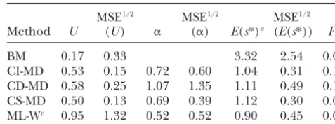
of the deleterious mutations, the deleterious effect is more TABLE 1
than mild (s⬎0.05). The case [U⫽ 5, ␣ ⫽0.5] could be
Pure model results for case 1
interpreted as at⫽25 MA experiment with ⫽0.2, where
ⵑ90% of the detectable deleterious mutations have only mild
MSE1/2 MSE1/2 MSE1/2 deleterious effects (s⬍0.05). These two cases are
approxi-Method U (U) ␣ (␣) E(s*)a (E(s*)) Fb mately representative of typical published estimates of viability
mutational parameters in Drosophila (seeGarcı´a-Doradoet
BM 0.17 0.33 3.32 2.54 0.00
al.1999), and they are more extensively explored.
CI-MD 0.53 0.15 0.72 0.60 1.04 0.31 0.17 As we use the scale parameter value () giving E|s|⫽
CD-MD 0.58 0.25 1.07 1.35 1.11 0.49 0.17 0.1/U, the average deleterious effect was 0.2 in the two cases
CS-MD 0.50 0.13 0.69 0.39 1.12 0.30 0.08 withU⫽0.5 and 0.02 in the two cases withU⫽5. However,
ML-Wc 0.95 1.32 0.52 0.52 0.90 0.45 0.00 because selection was absent, the magnitude of deleterious
effects is irrelevant to mutation accumulation. Since we setQ⫽
Estimates (averaged over replicates), and the square root 20 [whereQ⫽ 2G/2
Rand2G⫽tE(s2)], the scale forsis fixed
of their MSE, were obtained using different estimation meth-to giveE(s2)⫽Q2
R/t. In a real experiment,2R⫽ 2e/nε, where
ods on MA data simulated using the pure model withU ⫽ nεis the number of individuals assayed per line, and2eis the
0.5,␣ ⫽0.5, andQ⫽20. nongenetic variance of the fitness trait studied. Thus, using the
a|s|relative to the true expected simulated value. standard definition of mutational heritability (h2
m⫽ E(s2)/ b
Fraction of samples that failed to provide a global mini-(22e)), we obtain 2
R⫽ E(s2)/(2nεh2m), which implies 2G/
mum for the distance or a global maximum for the likelihood.
2
R⫽2nεth2mandnε⫽Q/(2th2m). c
Estimates were obtained by Keightley (1998) from 10 Ferna´ndezand Lo´ pez-Fanjul (1996) obtainedQ ⫽2.12
simulated MA lines and controls and are included here for for egg-to-adult viability after 105 MA generations, andQ ⬇
comparison. 3.6 was obtained for competitive viability in theMukaiet al.
(1972) data set (t⫽40) that has been analyzed by MD. We usedQ⫽20 (as assumed in mostKeightley1998 simulations) andQ⫽2 as reasonable bounds on the likely value ofQ.
coming can be due to the limited precision of the⌬M estimate but is partially overcome if the MD estimate of Numbers of replicates
⌬Mis allowed to vary two standard deviations around the For each case analyzed, 10 data sets were simulated, each empirically estimated⌬M. Thus, the control-supported consisting of 200 MA lines and 200 control lines. An exception
(CS)-MD analysis is a good choice to incorporate reli-is the caseU⫽0.5,␣ ⫽0.5,Q⫽20 (the first case we analyzed)
able empirical information on⌬M. for which two additional data sets were simulated after two
analyses failed to produce global MD estimates. For the re- On the whole, MD showed no bias for U or E(s*) maining cases no additional data were simulated to replace estimates. One exception is the case withU⫽ 5, ␣ ⫽ MD failures. Overall, 152 data sets were simulated, each subject 0.5, where an underestimate for
Uand an overestimate to several analyses as shown in the tables. Some additional
forE(s*) were obtained, the bias being always smaller ML-W estimates were obtained fromKeightley(1998, see
than those observed for BM. Furthermore, the caseU⫽ Table 5) and also correspond to 10 replicates (each with 200
MA and 200 control lines) per parameter set. 5,␣ ⫽ 0.5 with Q ⫽ 2 is the only one where CS-MD estimates had MSE smaller than that of the CI-MD, for bothUandE(s). This is not surprising, as largeUand RESULTS
smallQrender the distribution of the means of the MA lines more similar to a normal curve, masking the high
Pure model data: Results of different estimation
kurtosis of the distribution of effects and increasing the methods (BM, MD, and ML) from pure model
simu-relevance of the information about ⌬M. In any case, lated data are given in Tables 1–5. ML-W estimates
ob-the bias was always relatively small. tained byKeightley(1998) are included for
compari-For all the pure model cases where no advantageous son. To allow direct comparison with Keightley’s ML-W
mutations were simulated (those in Tables 1–4), MD results, we refer to the estimated expected absolute
ef-estimates forPa averaged 0.02. For cases with Q⫽ 20, fect on the trait (Eˆ|s|⫽ ␣ˆ/ˆ , where the hat stands for
90% of analyses gave Pa ⬍ 0.05, but with Q ⫽ 2 this estimation), relative to the true expected value (E(s*)⫽
dropped to 78% (results not shown). Empirical stan-Eˆ|s|/E|s|). For cases simulated usingPa⫽0, very similar
estimates were obtained forE(s) andE|s|. dard deviations were of the order of the corresponding BM underestimatedUand overestimatedE(s*). The estimates. Table 5 allows us to compare estimates for biases were smaller for ␣ ⫽ 2 than for ␣ ⫽ 0.5, as the caseU⫽0.5,␣ ⫽2,Q⫽20 for MA data simulated expected since the BM bounds became closer to the with Pa ⫽ 0 or Pa⫽ 0.1. The quality of BM estimates true parameter with decreasing coefficient of variation decreases with Pa ⬎ 0, as expected. MD estimates for Pawere reasonable but had large standard deviations, ofs, which is equal to 1/
√
␣in the gamma distribution.indicating thatPavalues ofⵑ0.05 can pass undetected MD estimates were generally less biased and had
in an MD analysis. The MSEs of MD estimates for U, smaller MSE than BM estimates, the difference being
␣, and E(s*) obtained by assuming no advantageous larger for small␣, as expected. The control-determined
mutations [Pa ⫽ 0 (PA0)-MD in Table 5] were not (CD)-MD analysis was not usually the best MD
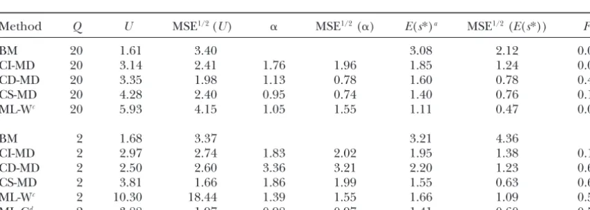
TABLE 2
Pure model results for case 2
Estimation
method Q U MSE1/2(U) ␣ MSE1/2(␣) E(s*)a MSE1/2(E(s*)) Fb
BM 20 0.34 0.20 1.54 0.69 0.00
CI-MD 20 0.46 0.10 2.34 1.01 1.05 0.19 0.00
CD-MD 20 0.55 0.14 2.47 2.16 0.93 0.25 0.10
CS-MD 20 0.50 0.13 1.88 0.76 0.97 0.19 0.00
ML-Wc 20 0.65 0.30 1.66 0.91 0.87 0.25 0.00
BM 2 0.36 0.19 1.37 0.61
CI-MD 2 0.41 0.17 3.80 2.58 1.12 0.24 0.10
CD-MD 2 0.70 0.86 2.56 1.70 0.81 0.92 0.10
CS-MD 2 0.46 0.24 3.78 2.46 1.10 0.32 0.10
ML-Wc 2 0.67 0.44 3.89 5.20 0.90 0.36 0.10
ML-Cd 2 1.93 4.32 3.04 3.52 0.83 0.46 0.00
Estimates (averaged over replicates), and the square root of their MSE, were obtained using different estimation methods on MA data simulated using the pure model withU⫽0.5 and␣ ⫽2.
a|s|relative to the true expected simulated value.
bFraction of samples that failed to provide a global minimum for the distance or a global maximum for the likelihood.
cEstimates for the case2G/2
R⫽20 are fromKeightley(1998) and also correspond to 10 simulated MA lines and controls.
dEstimates were obtained from our 10 simulated MA lines and controls using the true original mean and
2
Ras a known parameter.
for samples simulated withPa⫽0 and were larger when estimatePashould be preferred whenever there is uncer-tainty of whetherPais zero.
the samples had been simulated usingPa⫽0.1.
Further-more, when data were simulated using Pa ⫽ 0.1, the ML analysis showed a tendency to overestimate U. This seems to be due to a few very large estimates, analysis assumingPa⫽0 often produced no global
esti-mates. Thus, the general analysis allowing the user to despite the fact that the maximum was not searched for
TABLE 3
Pure model results for case 3
Method Q U MSE1/2(U) ␣ MSE1/2(␣) E(s*)a MSE1/2(E(s*)) Fb
BM 20 1.61 3.40 3.08 2.12 0.00
CI-MD 20 3.14 2.41 1.76 1.96 1.85 1.24 0.00
CD-MD 20 3.35 1.98 1.13 0.78 1.60 0.78 0.40
CS-MD 20 4.28 2.40 0.95 0.74 1.40 0.76 0.10
ML-Wc 20 5.93 4.15 1.05 1.55 1.11 0.47 0.00
BM 2 1.68 3.37 3.21 4.36
CI-MD 2 2.97 2.74 1.83 2.02 1.95 1.38 0.10
CD-MD 2 2.50 2.60 3.36 3.21 2.20 1.23 0.60
CS-MD 2 3.81 1.66 1.86 1.99 1.55 0.63 0.60
ML-Wc 2 10.30 18.44 1.39 1.55 1.66 1.09 0.50
ML-Cd 2 3.88 1.97 0.98 0.97 1.41 0.60 0.50
Estimates (averaged over replicates), and the square root of their MSE, were obtained using different estimation methods on MA data simulated using the pure model withU⫽5 and␣ ⫽0.5.
a|s|relative to the true expected simulated value.
bFraction of samples that failed to provide a global minimum for the distance or a global maximum for the likelihood.
cEstimates for the case2G/2
R⫽20 are fromKeightley(1998) and also correspond to 10 simulated MA lines and controls.
dEstimates were obtained from our 10 simulated MA lines and controls using the true original mean and
2
TABLE 4 true parameter value”) is 5.95 times larger than that for CS-MD. However, Keightley’s ML program and our MD Pure model results for case 4
program do not allow the comparison of both methods under identical conditions. The ML program maximizes MSE1/2 MSE1/2 MSE1/2
the joint likelihood of the MA and control samples, Method U (U) ␣ (␣) E(s*)a (E(s*)) Fb
allowing the user to specify0and2
Ras known values
BM 3.33 1.74 1.52 0.57 0.00
(ML-C analyses). Then, the estimate for ⌬M is condi-CI-MD 4.97 1.6 2.15 1.80 1.00 0.30 0.00
tioned on, but not determined by, the assumed0value. CD-MD 6.56 2.36 3.20 3.61 0.85 0.29 0.10
The MD program uses only the MA sample, although CS-MD 7.06 2.92 2.30 2.16 0.80 0.36 0.00
we can incorporate information from the control mean ML-Wc 7.70 6.73 2.98 3.65 0.87 0.33 0.10
(vc) to bound the⌬Mestimate or to set this at a given Estimates (averaged over replicates), and the square root
constant (CS or CD alternatives). Since in the MD analysis of their MSE, were obtained using different estimation
meth-reported here we have introduced the true2
Ras known, ods on MA data simulated using the pure model withU⫽5,
␣ ⫽2, andQ⫽20. the fair comparison is that between ML-C (where2 Ris set a|s|relative to the true expected simulated value.
at its true value and0 is set atvc) and a MD alternative bFraction of samples that failed to provide a global
mini-that incorporates information aboutvcwithout determin-mum for the distance or a global maxidetermin-mum for the likelihood.
ing a fixed⌬M. One such alternative (not necessarily the cEstimates were obtained by Keightley (1998) from 10
best one) is the CS-MD analysis using a 2-SE interval simulated MA lines and controls and are included here for
around⌬M. Relative MSE1/2averaged over cases in Tables comparison.
2 and 3 gives 4.51 for ML-C estimates ofUand 0.39 for CS-MD ones, so that average relative MSE1/2 for U is 11 times larger for ML-C than for CS-MD estimates. U⬎50. Thus, one of the ML-C analyses in Table 2 gave Removing an outlier ML-C estimate givingU⫽ 13, the U ⫽ 13, and one ML-W analysis in Table 3 gaveU ⫽ average relative MSE1/2forUis just 4.6 times larger for 42, these cases being insensitive to the starting position ML-C than for CS-MD estimates. MSE1/2’s for E|s| using in the search algorithm. This could be ascribed to the ML or CS-MD were roughly similar on average.
finding of maxima in regions where the likelihood pro- Although for a fair comparison with the MD analysis file is too flat, which might be due to the use of the of our simulated data the appropriate choice is ML-C, simplex algorithm to maximize the likelihood. Again, the difference between ML-W and ML-C was negligible the exception is the case U ⫽ 5, ␣ ⫽ 0.5 (Table 4), when they were computed for the same data sets. where ML-W overestimatesE(s*) and, after the outliers All this suggests that, when the analyzed data match are removed, underestimatesU, as occurred in the MD the model assumed in the MD or ML analysis, MD allows analysis. good estimation in the absence of a control assay and ML estimates for U had MSEs larger than those ob- that differences between ML and MD estimates could tained using CI- or CS-MD estimation (Tables 1–4). For be due to differences in the number of estimated param-example, the average over all ML estimates in Tables 1–4 eters, the nature of the data used (MA and controlvs.
only MA data), and/or the searching algorithms. of the relative MSE1/2 (i.e., the average of the “MSE1/2/
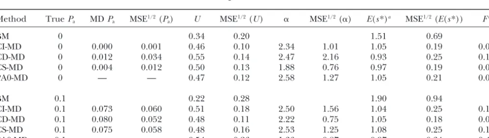
TABLE 5
Effect of thePavalue on the estimates
Method TruePa MDPa MSE1/2(Pa) U MSE1/2(U) ␣ MSE1/2(␣) E(s*)a MSE1/2(E(s*)) Fb
BM 0 0.34 0.20 1.51 0.69
CI-MD 0 0.000 0.001 0.46 0.10 2.34 1.01 1.05 0.19 0.00
CD-MD 0 0.012 0.034 0.55 0.14 2.47 2.16 0.93 0.25 0.10
CS-MD 0 0.004 0.012 0.50 0.13 1.88 0.76 0.97 0.19 0.00
PA0-MD 0 — — 0.47 0.12 2.58 1.27 1.05 0.21 0.00
BM 0.1 0.22 0.28 1.90 0.94
CI-MD 0.1 0.073 0.060 0.51 0.18 2.50 1.56 1.04 0.25 0.10
CD-MD 0.1 0.080 0.052 0.48 0.11 2.22 0.75 1.05 0.18 0.00
CS-MD 0.1 0.075 0.058 0.48 0.16 2.53 1.25 1.08 0.25 0.10
PA0-MD 0.1 — — 0.54 0.26 1.36 0.87 0.97 0.34 0.40
Estimates (averaged over replicates), and the square root of their MSE, were obtained using different MD estimation methods on MA data simulated using differentPavalues (pure model withU⫽0.5,␣ ⫽2, andQ⫽20).
a|s|relative to the true expected simulated value.
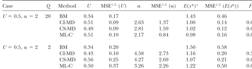
TABLE 6
Estimates for residual contaminated data
Case Q Method U MSE1/2(U) ␣ MSE1/2(␣) E(s*)a MSE1/2(E(s*)) Fb
U⫽0.5,␣ ⫽2 20 BM 0.34 0.17 1.43 0.46
CI-MD 0.51 0.09 2.63 1.37 1.00 0.14 0.00 CS-MD 0.49 0.09 2.81 1.59 1.02 0.12 0.00 ML-Cc 0.51 0.10 2.17 0.84 0.98 0.16 0.00
U⫽0.5,␣ ⫽2 2 BM 0.34 0.20 1.50 0.58
CI-MD 0.43 0.10 4.58 2.73 1.16 0.20 0.30 CS-MD 0.56 0.25 4.27 2.69 1.07 0.21 0.00 ML-Cc 0.50 0.37 3.26 2.26 1.22 0.50 0.00
Estimates (averaged over replicates), and the square root of their MSE, were obtained using different estimation methods on MA data simulated using the residual contaminated model for the two more representa-tive parameter sets.
a|s|relative to the true expected simulated value.
bFraction of samples that failed to provide a global minimum for the distance or a global maximum for the likelihood.
cEstimates were obtained from our 10 simulated MA lines and controls using the true original mean and
2
Ras known parameter.
Both ML and MD showed a trend to moderately over- was more likely to occur under large U and small Q, when the distribution of the trait mean in the lines is estimate␣, although, in all cases, the true parameter value
was included within two standard deviations around the expected to be closer to normality and, therefore, less informative.
corresponding estimate. Therefore, individual estimates
are not expected to significantly differ from the true Effect of nonnormal residual errors: The empirical distribution of the per-vial random deviations (d) had parameter values (note that the standard deviation
be-tween replicate estimates would correspond to the stan- skewness coefficient⫺0.47. This distribution and that forR(fornε⫽3) significantly departed from normality
dard error of individual estimates obtained in a single
data set or experiment). For both MD and ML analyses, (p⬍0.1%).
Table 6 gives results of BM, MD (CI and CS), and theU andE(s*) estimates were largely insensitive to␣
above some threshold value around 10 or 20. It should ML-C analyses on data simulated following the residual contaminated model, for the two more representative be remembered that both the kurtosis coefficient and
the coefficient of variation of a gamma distribution as- cases. All but one of the estimates (BM, MD, or ML) showed smaller MSE than those obtained under the ymptotically decrease with increasing␣, so that large␣
differences (or large MSE for ␣ estimates) can be analogous pure model, irrespective of the U, ␣, or Q values used to simulate the data. Although we do not scarcely relevant for large ␣values. In a few data sets,
the ML profile plotted against ␣ increased up to the have an explanation for this unexpected result, it may be due to sampling error, as there happened to be no maximum value we used to build the ML profile (␣ ⫽
20). For these cases, a constant-effect model (equivalent outliers in the case of ML-C, which partly explains the lower MSE.
to␣ ⫽∞) showed a slightly larger maximum likelihood
than the␣ ⫽20 gamma model showed, but the estimates Detection of mutations with small deleterious effect:
With gamma-simulated deleterious effects, the case U⫽ forUandE(s) remained the same under both models
(gamma or constant effects). These data sets were used 5, ␣ ⫽0.5 implies a high rate of mutation with mild deleterious effects (Us⬍0.05⫽4.34). CI-MD as well as both to compute the average ML estimates for UandE(s*)
but are excluded in the computation of the average␣ ML analyses detects more than half of these (Table 3). On average, MD detectedⵑ70% of the simulated delete-estimate.
A problem common to both ML and MD analyses is rious mutation rate, ML gave overestimates due to out-lierUvalues, and BM estimated a mutation rateⵑ30% that, on occasion, they do not provide a global
maxi-mum for the likelihood (or a global minimaxi-mum for the of the simulated one. Both ML and MD estimates of the average effect were more accurate than BM estimates. distance), corresponding to a set of parameter
esti-mates. This occurred with similar frequencies under CI- When constant-effect mildly deleterious mutations were added to the U ⫽ 0.5, ␣ ⫽ 2 pure model case MD, CS-MD, ML-W, or ML-C, but in different data sets.
It was more common in CD-MD analysis. In those occa- (mild contaminated model), both the BM and the CI-MD analyses underestimateUand overestimateE|s| (Ta-sions, the distance profile decreased (or the likelihood
TABLE 7
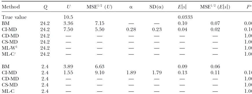
Estimates for mild contaminated data
Method Q U MSE1/2(U) ␣ SD(␣) E|s| MSE1/2(E|s|) Fa
True value 10.5 0.0333
BM 24.2 3.36 7.15 — — 0.10 0.07 0.00
CI-MD 24.2 7.50 5.50 0.28 0.23 0.04 0.02 0.10
CD-MD 24.2 — — — — — — 1.00
CS-MD 24.2 — — — — — — 1.00
ML-Wb 24.2 — — — — — — 1.00
ML-Cc 24.2 — — — — — — 1.00
BM 2.4 3.89 6.63 0.09 0.06
CI-MD 2.4 1.55 9.10 1.89 1.79 0.13 0.11 0.10
CD-MD 2.4 — — — — — — 1.00
CS-MD 2.4 — — — — — — 1.00
ML-C 2.4 — — — — — — 1.00
Estimates (averaged over replicates) for the different parameters and the square root of their MSE from MA data simulated using the mild contaminated models for U⫽ 0.5 and␣ ⫽2 are shown (SDs are given instead of MSE in the case of␣, as the expected␣value is not defined for the mild contaminated model).
aFraction of samples that failed to provide a global minimum for the distance or a global maximum for the likelihood.
bEstimates, including those of the original average and2R, obtained from our 10 simulated MA lines and controls.
cEstimates obtained from our 10 simulated MA lines and controls using the true original mean and2 Ras known parameter.
irrespective of the data precision (i.e., for bothQ⫽24 mates, which depend upon the control average and, therefore, upon the control-based ⌬M estimate. The andQ ⫽ 2.4), although it estimates an average effect
(E(s)⫽0.10) that is very different from the mild con- fact that no estimates are found whenUE(s) is forced to its true value suggests that no gamma distribution taminant effect (E(s)⫽0.025), from the average effect
of the uncontaminated gamma distribution (E(s)⫽0.2), both reasonably fits the gamma contaminated distribu-tion and produces the true overallUE(s) value. and from the true average of the contaminant-gamma
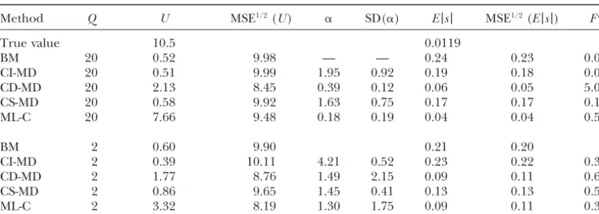
mixed distribution (E(s) ⫽ 0.0333). In contrast, the For the tiny contaminated model (Table 8), BM, CI-MD, and CS-MS did not allow us to detect the additional quality of MD estimates depends upon the data assay
precision. For large Q, CI-MD estimates were clearly rate of tiny mutations, irrespective of the assay precision. Estimates constrained to the observed⌬M(CD-MD or better than BM estimates. Besides showing considerably
smaller MSE, CI-MD detectedⵑ71% of the total muta- ML-C) account for larger fractions of the tiny-contami-nant class when assay precision is large, suggesting that tion rate and gave good estimates of the average
deleteri-ous effect. Although the constant-effect mild contami- gamma distributions with low␣may account better for tiny contaminant effects than for mild effects. However, nants are not modeled by the gamma distribution, CI-MD
estimated a gamma distribution where the frequency of although ML-C estimates ofUandE|s|are reasonable whenQ⫽20, the difference between methods is scarcely the mild-effect class accounts forⵑ50% of the
contami-nant “mild” mutations, and this was attained making relevant due to the very large MSE1/2values. These values were about as large as or larger than the true parameter. no use of the control-based ⌬M estimate. Due to the
assumption of gamma-distributed effects, this MD detec- Therefore, estimates do not significantly differ from zero, from the true value, or from the estimate obtained tion of a fraction of mild contaminant mutations was
obtained at the expense of overestimating the rate of using an alternative method. Furthermore, about one-half the cases provided no global estimates.
moderately deleterious mutation (see Figure 1). With low Q, CI-MD becomes even less efficient than BM, detecting only ⵑ15% of the total mutation rate, BM
DISCUSSION and MD estimates for U being of the same order of
magnitude. Surprisingly, when the control-based ⌬M For pure model simulated data, both ML and MD esti-mates for the total mutation rate (U) and the average estimate was incorporated (i.e., in CD or CS-MD
analy-sis) none of the samples provided global point estimates deleterious effect (E|s|) were less biased than BM esti-mates, as expected. CI-MD was among the better choices, for the parameters (i.e., no global minimum for the
obtained MSE values for ML estimates of Uthat were slightly smaller than those for BM estimates (see cases evaluated at generations 0 and 80 in Table 2 from KeightleyandBataillon2000). Thus, a ML analysis based on a simpler, although less appropriate, model may work better. This suggests that the common occur-rence of outliers in estimates ofUobtained by ML under the gamma model may be due to difficulties in maximiz-ing over too many parameters and/or in the search algorithm used in the programs.
Both ML and MD analyses gave reasonable estimates for the shape parameter ␣, although these estimates were highly variable with large ␣values, exhibiting an upward bias and high MSE. However,U andE(s) esti-mates were very insensitive to variation in ␣once␣ is large. This could be ascribed to the fact that the shape of the gamma distribution becomes quite stable to varia-tion in␣when when␣is large.
For pure model data, the precision of the estimates is not greatly affected by the precision with which the trait mean is assayed (Q ⫽ 2
G/2R). However, the proba-bility of finding MD or ML global estimates with Q ⫽ 20 is, on average, about four times larger than that with Figure 1.—Expected number of mutations accumulated Q⫽ 2.
per line plotted against deleterious effect (grouped in 0.05
For ML estimates, asymptotic 95% support limits can width classes) for the “mild contaminated” model.
be computed on the basis of a drop in natural log likeli-hood of two from the maxima in the likelilikeli-hood profiles (see Keightley 1994). The distribution of the Cramer-von Mises distance (W2) between the empirical (Fn) and information. To incorporate the control-based estimate
of the mutational rate of viability decline (⌬M), CS-MD the true distribution (F) does not depend onF
when-everFis continuous (i.e., it is distribution free), but only
estimates should be preferred to CD-MD ones, since the
latter are associated with larger MSE and with a larger on the sample sizen. Since, forn⬎20, the probability of a distanceW2⬎0.46 isⵑ0.05 (Scott2000), the set of proportion of distance profiles showing no minimum.
Although the MD power to estimate the rate of favorable parameter values associated withW2⬍0.46 define a 95% credible interval, analogous to that defined by the ML mutation (Pa) is poor, it is convenient to simultaneously
estimate this parameter to prevent any bias in the esti- support limits. This can be straightforwardly computed from the distance profile. In both cases (ML and MD), mates of␣,U, andE(s). This result is model dependent,
and we have not checked the behavior of our MD esti- credible intervals are very wide, often being of infinite length. However, it should be noted that these credible mates in cases where favorable effects are not obtained
from a reflected-gamma distribution.Shawet al.(2002) intervals are not standard confidence intervals, but in-tervals of parametric values that could not be rejected have recently published a ML alternative for a model
where favorable mutations are simulated by displacing in a goodness-of-fit test. Standard confidence intervals do not depend on the distribution of the W2 distance a gamma distribution of deleterious effects. Simulation
showed that the method is efficient when the displace- itself, but on the distribution of the MD estimates (theˆ value that minimizesW2) as a function of the true parame-ment is known. Therefore, information on the
distribu-tion of favorable mutadistribu-tions for fitness traits (which are ter value (). Unfortunately, the distribution of MD estimates is unknown, although it can be approached not necessarily favorable for overall fitness) is required
to choose the more appropriate estimation model. using bootstrap. Analogously, a confidence interval for ML estimates would not depend on the distribution of Pure model ML estimates occasionally gave large
out-lier U values, causing MSE1/2 and SD for U up to 10 the likelihood itself, but on the distribution of the ML estimates. If, for a given true, MD (or ML)ˆ estimates times those for MD estimates and considerably
ex-ceeding the BM ones. As ML is asymptotically efficient have a high probability of being close to, confidence intervals should be small. However, W2 could still be under some regularity conditions (Van der Vaart
1998, pp. 65 and 120), larger SD values were unex- relatively small (or the likelihood relatively high) for parameter values well outside the confidence interval, pected. However, it should be noted that Keightley and
TABLE 8
Estimates for tiny contaminated data
Method Q U MSE1/2(U) ␣ SD(␣) E|s| MSE1/2(E|s|) Fa
True value 10.5 0.0119
BM 20 0.52 9.98 — — 0.24 0.23 0.00
CI-MD 20 0.51 9.99 1.95 0.92 0.19 0.18 0.00
CD-MD 20 2.13 8.45 0.39 0.12 0.06 0.05 5.00
CS-MD 20 0.58 9.92 1.63 0.75 0.17 0.17 0.10
ML-C 20 7.66 9.48 0.18 0.19 0.04 0.04 0.50
BM 2 0.60 9.90 0.21 0.20
CI-MD 2 0.39 10.11 4.21 0.52 0.23 0.22 0.30
CD-MD 2 1.77 8.76 1.49 2.15 0.09 0.11 0.60
CS-MD 2 0.86 9.65 1.45 0.41 0.13 0.13 0.50
ML-C 2 3.32 8.19 1.30 1.75 0.09 0.11 0.30
Estimates (averaged over replicates) for the different parameters and the square root of their MSE from MA data simulated using the tiny contaminated models forU⫽0.5 and␣ ⫽2 (SDs are given instead of MSE in the case of␣, as the expected␣value is not defined for the tiny contaminated model).
aFraction of samples that failed to provide a global minimum for the distance or a global maximum for the likelihood.
that the asymptotic validity of ML errors (as well as the evaluation of a reliable control population (see Equa-tion 3) and that this might explain why CI-MD mutaEqua-tion ML asymptotic efficiency) depends on specific
assump-tions that are not trivial (Van der Vaart1998, pp. 65 rates estimated from the Mukai et al. (1972) data by ignoring the control information were only 8% of the and 120) and have not been checked even under the
pure model. Even if those assumptions were met, the BM estimates obtained using such⌬M(Garcı´a-Dorado et al.1999; Lynchet al. 1999). However, for the pure validity of MD or asymptotic ML credible intervals
de-pends on the variable being drawn from the distribution model with U ⫽ 5, ␣ ⫽ 0.5, and E(s) ⫽ 0.02 (which gives a mild mutation rate of Us⬍0.05 ⫽ 4.35), CI-MD assumed by the model. All this considered, errors or
confidence intervals based on bootstrapping, which are average estimates forUs⬍0.05(2.35 or 2.18 forQ⫽20 or Q⫽2, respectively) were larger than the BM bounds for more directly interpretable, should be preferred if the
corresponding computational effort can be undertaken. totalU(1.61 or 1.68 forQ⫽20 orQ⫽2, respectively). Furthermore, the rate of mean decline (⌬MCI-MC) pre-It would be worth exploring the properties of
bootstrap-ping in a future study. dicted from CI-MD is fairly accurate (94 and 90% of the simulated decline forQ⫽20 orQ⫽2, respectively). Using sampling residuals estimated from Drosophila
viability assays (instead of normally distributed ones) On the other hand, it has been noted (Garcı´a -Dorado1997) that a high rate of mutations with “small” did not have an appreciable effect on the estimates and
their MSEs (BM, MD, or ML), even when the residual deleterious effects, not fitting the gamma distribution assumed fors, could pass undetected in a CI-MD analy-variance was large (Q ⫽ 2) and only nε ⫽ 3
single-female sampling errorsd were averaged per MA line sis. To check this possibility, MA data were simulated using mild contaminated or tiny contaminated models, (d, estimated fromFerna´ndezandLo´ pez-Fanjul1996
data). This result suggests that MD estimates based on where the distribution of deleterious effects departed from a gamma distribution due to a very common class the Ferna´ndez and Lo´pez-Fanjul data (Garcı´a-Dorado
1997) are unlikely to be biased due to nonnormal resid- of deleterious mutations with constant small effect. It must be noted that even the continuity assumption is uals, asnε⫽12dvalues were averaged in those data to
assay the viability of each line. Thus, due to the central violated in this contaminated model.
For the mild contaminated model, BM detected only limit theorem, they should have a distribution closer to
a normal curve. However, this conclusion cannot be ⵑ35% of the deleterious mutation rate, and the CD-MD or ML-C methods, constrained to produce exactly extrapolated to residuals with other unknown
nonnor-mal distributions, and strongly asymmetric distributions the observed change in the mean relative to the control, usually failed to produce global estimates for all the may induce estimation bias.
It has been proposed that detecting common deleteri- parameters. In contrast, a substantial fraction of mild contaminants is detected by CI-MD (i.e., in the absence ous mutations with small effect requires an estimate
were assayed with high precision (Q⫽20). In this case, fore, the optimal MA period depends on the mutation rate.
CI-MD analysis detects 71% of the simulated mutation
In the absence of a priori information on the true rate, estimates a gamma distribution of s close to the
deleterious mutation rate, it could be convenient to true mild contaminant-gamma mixed distribution
(Fig-assay the trait more than once during the MA experi-ure 1), and accounts for more than half of the
muta-ment, until estimates can be obtained with reasonable tional decline in mean. With low precision data (Q ⫽
precision. Incorporating data from multiple genera-2), CI-MD becomes even less efficient than BM,
de-tions in an ML framework has proven to be more effi-tecting only ⵑ15% of the deleterious mutation rate.
cient than incorporating data from single-generation Even then, BM and CI-MD estimates are of the same
ML for a constantsmodel (KeightleyandBataillon order (UBM/UCI-MD⫽ 2.5). This suggests that the large
2000). However, the gain in precision should be differences between these estimates found forMukaiet
weighed against the increased experimental effort re-al.(1972) data (UBM/UCI-MD⫽13) should not be ascribed
quired for repeated evaluation. A multigeneration ML to CI-MD missing mild deleterious effects not fitting into
method for a gamma-s model has been developed by the gamma distribution (Garcı´a-Doradoet al. 1998).
Shawet al.(2002). Although the procedure is cumber-The above results show the convenience of checking
some, it might be worth studying the relative efficiency the agreement between the CI-MD-estimated UE(s)
of a multigeneration analysis. value and a⌬Mestimate on the basis of comparison to
We have found that single-assay data, analyzed by CI-a reliCI-able control, which would support the vCI-alidity of
MD and CS-MD, can provide accurate information if the MD estimates. This is particularly useful for
low-the trait is assayed when most lines have accumulated precision data. Even when the MA means have been
a small number of deleterious mutations. This requires assayed with low precision, the findings of CD-MD
esti-MA lines and control (if available) being assayed as mates and their agreement with the CI-MD ones, as was
precisely as possible at the end of the MA period. These the case in the analysis of the Ferna´ndez and
Lo´pez-CI-MD and CS-MD estimates have relatively small MSEs Fanjul MA data (Garcı´a-Dorado 1997), suggest that
and are relatively robust against contamination with mu-the gamma model provides an adequate description of
tations of mild deleterious effects. ML can also be used the distribution of deleterious effects, including mild
if a reliable control assay is available, but some criterion ones. Finally, if CS-MD estimates can be obtained, they
should be developed to indicate whether the ML surface appear to be the best way to incorporate control
infor-is too flat, in which case the parameter estimates should mation into the analysis.
be ignored. Bootstrap errors can be obtained for MD No method, however, allowed reliable detection of a
or ML estimates. If both MD and ML fail to provide contaminant class of mutations with tiny effects.
Al-global estimates, BM bounds should be computed. though ML appeared to obtain reasonable average
esti-We are indebted to P. D. Keightley for kindly providing his ML
mates when the trait is assayed with high precision (Q⫽
program and to J. F. Crow, C. Lo´pez-Fanjul, and S. Otto for useful
20), individual estimates were highly variable, giving discussions of the manuscript. This work was supported by grant PB98-MSE1/2about the true parameter value being estimated.
0814-C03-01 from the Ministerio de Educacio´n y Cultura, Spain.
This confirms the view that MA experiments should not be intended to investigate mutations with extremely small effects (Garcı´a-Dorado 1997; Keightley and
LITERATURE CITED
Eyre-Walker1999).
Cao, R., A. CuevasandR. Fraiman, 1995 Minimum distance
den-Our conclusions refer to the analysis of data obtained
sity-based estimation. Comput. Stat. Data Anal.20:611–631.
from a single assay of a fitness trait in a MA experiment. Chavarrı´as, D., C. Lo´ pez-Fanjul and A. Garcı´a-Dorado,
2001 The rate of mutation and the homozygous and
heterozy-Denget al. (1999) found that BM estimates from a single
gous mutational effects for competitive viability: a long-term
ex-assay in 10-generation MA experiments achieved about periment with
Drosophila melanogaster. Genetics158:681–693.
the same quality as those from longer MA experiments. Deng, H.-W., J. LiandJ.-L. Li, 1999 On the experimental design and data analysis of mutation accumulation experiments. Genet.
However, this conclusion depends on the particular
mu-Res.73:147–164.
tational parameter values used in those simulations giv- Ferna´ndez, J., andC. Lo´ pez-Fanjul, 1996 Spontaneous mutational ing relatively large rates of mean decline, which can be variances and covariances for fitness-related traits inDrosophila
melanogaster.Genetics143:829–837.
efficiently estimated after a short MA period. On the
Garcı´a-Dorado, A., 1997 The rate and effects distribution of
viabil-other hand, ML and MD make use of the information ity mutation in Drosophila: minimum distance estimation. Evolu-contained in the observed shape of the distribution of tion51:1130–1139.
Garcı´a-Dorado, A., andJ. M. Marı´n, 1998 Minimum distance
esti-the means of esti-the linesf(v), which approaches normality
mation of mutational parameters for quantitative traits.
Biomet-as the expected number of mutations accumulated per rics54:1097–1114.
line (U⫽t) increases. After sufficiently long MA peri- Garcı´a-Dorado, A., J. L. Monedero and C. Lo´ pez-Fanjul, 1998 The mutation rate and the distribution of mutational
ef-ods,f(v) becomes virtually normal and uninformative.
fects of viability and fitness inDrosophila melanogaster.Genetica
At that time, neither ML nor MD global estimates are 102/103:255–265.
Garcı´a-Dorado, A., C. Lo´ pez-Fanjul and A. Caballero, 1999
There-Properties of spontaneous mutations affecting quantitative traits. Parr, W. C., andW. R. Schucany, 1988 Minimum distance and robust estimation. J. Am. Stat. Assoc.75:616–624.
Genet. Res.74:341–350.
Keightley, P. D., 1994 The distribution of mutation effects on Scott, W. F., 2000 Tables of the Cramer-von Mises distributions. Commun. Stat. Theory Methods29:227–235.
viability inDrosophila melanogaster.Genetics138:1315–1322.
Keightley, P. D., 1998 Inference of genome-wide mutation rates Shaw, F. H., C. J. GeyerandR. G. Shaw, 2002 A comprehensive model of mutations affecting fitness and inferences forArabidopsis
and distributions of mutation effects for fitness traits: a simulation
study. Genetics150:1283–1293. thaliana.Evolution56:453–463.
Titterington, D. M., A. F. M. SmithandU. E. Markov, 1985
Statis-Keightley, P. D., andT. M. Bataillon, 2000 Multigeneration
maxi-mum-likelihood analysis applied to mutation-accumulation ex- tical Analysis of Finite Mixture Distributions. John Wiley & Sons, New York.
periments withCaenorhabditis elegans.Genetics154:1193–1201.
Keightley, P. D., andA. Eyre-Walker, 1999 Terumi Mukai and Van Der Vaart, A. W., 1998 Asymptotic Statistics. Cambridge Univer-the riddle of deleterious mutation rates. Genetics153:515–523. sity Press, Cambridge, UK.
Keightley, P. D., andO. Ohnishi, 1998 EMS-induced polygenic Vassilieva, L. L., A. M. HookandM. Lynch, 2000 The fitness mutation rates for nine quantitative characters inDrosophila mela- effects of spontaneous mutations inCaenorhabditis elegans.
Evolu-nogaster.Genetics148:753–766. tion54:1234–1246.
Lynch, M., J. Blanchard, D. Houle, T. Kibota, S. Schultz, Woodward, W. A., W. C. Parr, W. R. SchucanyandH. Lindsley, 1999 Spontaneous deleterious mutation. Evolution 53: 645– 1984 A comparison of minimum distance and maximum likeli-663. hood estimation of a mixture proportion. J. Am. Stat. Assoc.79:
Mukai, T., S. I. Chigusa, L. E. MettlerandJ. F. Crow, 1972 Muta- 590–598. tion rate and dominance of genes affecting viability inDrosophila