Essays in Development and
Transition Economics
Inaugural-Dissertation
zur Erlangung des Grades
Doctor oeconomiae publicae (Dr. oec. publ.)
an der Ludwig-Maximilians-Universität
München
2005
vorgelegt von
Sitki Utku Teksöz
Referent:
Prof. Stephan Klasen, PhD.
Korreferent:
Prof. John Komlos, PhD
Essays in Development and
Transition Economics
Submitted to the Department of Economics
In partial fulfilment of the requirements for the degree of
Doctor oeconomiae publicae (Dr. oec. publ.)
at the Ludwig-Maximilians University, Munich
2005
by
Sitki Utku Teksöz
Supervisor:
Prof. Stephan Klasen, PhD.
Co-supervisor:
Prof. John Komlos, PhD
List of Tables
Table 2.1: Equilibrium by Scenario and Numerical Illustration
Table 2.2.a and b: Ordinary Least Squares: Gross and Net FDI Inflows Table 2.3: Total Variance Explained, Data on Corruption by the WEF 2003 Table 2.4: Coefficient Matrix, Data on Corruption by the WEF 2003
Table 2.5: OLS,Component 2: Grand Type of Corruption
Table 2.6.a and b: Ordinary Least Squares and Weighted Least Squares: Gross and Net FDI Inflows
Table 2.7.a and b: Ordinary Least Squares: Gross and Net FDI Inflows Table A.2.1: Description of the Data Used in the Study
Table A.2.2: Principal Components Used in the Study Table 3.1: Institutions in the Augmented Solow Model
Table 3.2: Direct and Indirect Contributions of Institutions to Per Capita Income Table 3.3: Institutional Effects on Labour and Capital Productivities
Table A.3.2.1: Descriptive Statistics Table A.3.2.2: First Stage Regressions
Table A.3.2.3: Institutions in the Augmented Solow Model (OLS)
Table A.3.2.4: Institutional Effects on Labour and Capital Productivities (OLS) Table 4.1: Average life satisfaction scores and percentiles by country
Table 4.2: Satisfaction equations (WVS wave four)
Table 4.3: Satisfaction equations with macroeconomic variables
Table 4.4: Satisfaction equations with macroeconomic and reform variables, Transition Sample
Table 4.5: Life Satisfaction through Time
Table 4.6: Satisfaction equations with two way fixed effects Table A.4.1: Description of the Data Used in the Study
List of Figures
Figure 1.1: The Link between Corruption, Capital Flows and Financial Crises Figure 2.1: Average Gross FDI and Corruption
Figure 2.2: Average Net FDI and Corruption
Figure 3.1: Output and the residual: growth accounting Figure 3.2: Output and the residual: the combined model Figure 3.3: Institutions and the residual: the combined model Figure 4.1: Real GDP Growth Transition Countries
Figure 4.2: Income vs Life Satisfaction
Acknowledgements
Chapter 1
Introduction
Della Porta and Vanucci (1999) start their book Corrupt Exchanges with this remarkable comment: “Corruption is one of the most acute expressions of triumphant democracy’s unresolved problems.” (p.4). Corruption is no doubt a multidimensional phenomenon, and this statement fails to do justice to the complex nature of the problem at hand. One should also add that corruption is neither a problem specific to our age, nor to triumphant democracy for that matter.1
Now that we know that corruption is a widespread and endemic problem, can it be rooted out? Theoretically, this may be possible. However, in how far this route of action would be desirable is subject to debate. Rooting out corruption completely has its own trade-offs. Certainly, corruption imposes sizeable costs on society. On the other hand, fighting corruption is also costly. One of the standard tools of the economics profession, the cost and benefit analysis, might dictate that fighting corruption fails to cover the resources spent and opportunities lost along the way after a certain point, i.e. there might be declining marginal returns to scale in fighting corruption. Hence, Klitgaard (1988) argues that the optimal level of corruption is not zero (pp.24-25).
We have already started talking about corruption, but the crucial question is: What is corruption actually? How do we define it? Defining corruption precisely is a challenge. It is indeed very difficult to reach a definition that is wide enough in its coverage, abstains from value judgements, and at the same time serves analytical
1
purposes. The most widespread definition of corruption among economists is as follows: “Corruption is the misuse of public power for private benefit.”2
Although it sounds rather straightforward, this definition suffers from a few shortcomings. For instance, the term “misuse” implies a deviation from the formal duties of a public position. Yet, a legal definition of this term fails to cover informal rules, the public’s expectations, codes of conduct etc. Moreover, the definition assumes implicitly the presence of a clear distinction between the public and the private spheres, which need not always be the case in every single country. What is more, the concept of private benefit is not always easy to lay down clearly in the complicated cases whereby what is exchanged is not necessarily cash, but rather intangible substances such as power, status, or a future promise. However, it needs to be recognised that what is offered here is a working definition that renders a coherent analysis of corruption possible. Furthermore, this definition of corruption is endorsed by international financial institutions (IFIs) such as the World Bank and the IMF, and non-governmental organisations (NGOs) such as Transparency International.3
What must be clear from the definition above is that corruption is a state-society relationship. At the international level, globalisation has increased opportunities for collusive and concealed transactions between foreign private actors and host governments. Some examples are multinational companies being engaged in buying concessions, monopolies, etc.; kickbacks being offered in handing out contracts and/or loans; development aimed projects made unnecessarily expensive due to excessive spending resulting from unnecessary travels, and purchase of new computers; and numerous fringe benefits for local officials. In general, when the discretion that the public servants enjoy is considerable, and the regulations are non-transparent such that these officials can not easily be held accountable for their deeds, corruption becomes more likely. According to Andvig and Fjeldtad (2000), the problem common to all of these cases mentioned above is that corruption tends to
2
Senturia, J A., “Corruption, Political” Encyclopaedia of the Social Sciences, vol. 4 (New York: Crowell-Collier-Macmillian, 1930-1935). However, similar definitions are common to most economists and policy makers.
3
levy hidden costs on public services and blurs the distinction between the public and private spheres.
To clarify the concept of corruption, Tanzi (1995, pp.161-162) defines the arm’s length principle, which dictates that personal or other relationships should play no role regarding economic decisions. His approach to defining corruption is heavily influenced by the Weberian legal-rational paradigm of public office, organised on the basis of rational procedures and universal principles, granting no room for personal motives. Corruption is, then, defined as failure to respect the distinction between public and private, or alternatively to break the arm’s length principle, hence creating fertile ground for the seeds of corruption. However, this notion of public office is not immune to criticism, either. First of all, it was stated that public office is a western concept which need not find its exact equivalent in other societies. The second point regarding Weberian influenced conceptions of corruption is that legal procedures are not necessarily rational.4
The obvious conclusion is that a discussion of the definitions of corruption is not actually a fruitful one. Indeed, corruption is a difficult concept to define, yet an easy one to recognise. Johnston (1989, pp.92) summarises this point elegantly:
Despite the fact that most people, most of the time, know corruption when they see it, defining the concept does raise difficult theoretical and empirical questions. We are unlikely ever to arrive at a single definition, which accurately identifies all possible cases. Moreover, if a significant proportion of the population regard a person, process, or regime as corrupt, or if they believe that corruption is inevitable in their daily lives, that is an important social and political fact, whatever an analyst might say about the situation.
For the purposes of the present study, the distinction between grand corruption and petty corruption needs to be clarified. Grand corruption, also known as political corruption, is the type of corruption observed at the highest levels of political authority. Grand corruption involves the corruptness of the decision-making segments of the society, as in cases where politicians exploit their positions for private gain, e.g., by receiving kick backs from the contracts that the state hands out, or the embezzlement of large sums from the public resources.5
4
See Andvig and Fjeldstad (2000, pp.65-66). 5
The definition of petty corruption follows straight from that of grand corruption. Also known as bureaucratic corruption, petty corruption is corruption at the public administration level, rather than at the decision-making end of politics. This is the lower level corruption that a typical citizen experiences in daily life, as in when they have to pay bribes in their encounters with public servants either to receive a service, or to escape from punishment. The difference between the two forms of corruption may not always be evident in real life situations as these could be mutually reinforcing in a pyramid of upward extraction. However, on the analytical level, the distinction lies in the fact that petty corruption is a deviation from written rules, or implicit codes of conduct, whereas the extent of grand corruption exceeds this by far. Grand corruption covers abusing, sidestepping, ignoring or tailoring laws and regulations to secure private gain.6
There are certainly many methodologies that could be employed to analyse corruption. Perspectives from political science, psychology, sociology and anthropology all provide important insights for analysis. The advantage of putting this topic in an economic framework enables us to take a step away from fatalistic and moralistic explanations about the phenomenon, and to treat it in a value neutral manner. Given the policy implications, it probably would not be an overstatement to say that an understanding of the economic treatment of this problem will be central to keeping a firm stand on this very slippery ground. For instance, one tends to associate corruption somehow with a lack of morals or ethics, or by the breaking of the laws in the everyday usage of the term. However, as far as the economic analysis is concerned, there are strong differences between the terms “corrupt”, “illegal”, “unethical”, and “immoral”, hence they can not be used interchangeably. That is, not all illegal transactions are corrupt and vice versa. The same argument holds for unethical and immoral transactions, too.7 To tie up this discussion with the words of Rose-Ackerman (1999, p.xi): “Cultural differences and morality provide nuance and subtlety, but an economic approach is fundamental to understanding where corrupt incentives are the greatest and have the biggest impact.”
Chapter II of this manuscript presents a predominantly empirical analysis of the relationship between corruption and foreign direct investment (FDI). The empirical
6
See Andvig and Fjeldstad (2000, p.19). This point also strengthens the earlier caveat about the dangers of relying only on the criteria of deviation from formal legal rules in order to define corruption. 7
work on corruption goes back to the seminal paper of Mauro (1995), which concludes that corruption is harmful for growth, and that this channel mainly operates through its negative impact on investment.8 There are already a number of studies on the impact of corruption on FDI (Habib and Zurawicki, 2001 and 2002; Wei and Wu, 2001; Smarzynka and Wu, 2000, etc.). By now, it can be stated that corruption has a negative impact on foreign direct inflows. To put the study into a big picture, one needs to think of the linkages in Figure 1.1.
Figure 1.1 The Link between Corruption, Capital Flows and Financial Crises
The broad argument can be summarised as follows: The presence of corruption in a country distorts the composition of capital flows against foreign direct investment, and in favour of more volatile forms of capital flows such as portfolio investments and bank loans as depicted by the first arrow in the flow chart in Figure 1.1. The argument then follows that such a volatile composition of capital flows that is relatively weak on FDI increases the likelihood of currency/financial crises, as depicted by the second arrow. This latter link is relatively well-researched (Frankel and Rose, 1996; Radelet and Sachs, 1998; Rodrik and Velasco, 1999). Hence, we turn our attention to the former link in chapter II.
The novelty of the analysis in chapter II is to take an in-depth look into the survey data on corruption in order to differentiate between different types of
8
By virtue of being the first empirical treatment of corruption, this paper has also said the final word on the long-lasting debate on whether corruption greases the wheel (see Leff (1964) and Huntington (1968) for example), or it is sand in the wheels (see Myrdal (1968)).
Corruption
A particular composition of capital flows (relatively light on FDI)
corruption. Running a principal components analysis with the data on the available seven subcomponents of corruption, two principal components are retained, pertaining to the level of corruption (component 1) and to the type of corruption (component 2). This approach solves the problem of multicollinearity and allows us to distinguish between the grand and petty types of corruption. The chapter concludes that between petty and grand corruption, foreign investors are deterred more by the latter type of corruption. The chapter also offers theoretical reasoning why this might be the case and ends with policy implications.
Moving from chapter II to III, we turn our attention away from the specific field of corruption, which is but one of the manifestations of institutional failure, and focus on the institutions and growth linkages. To explain the basics of this argument, let us first start with a definition of institutions. North (1990) defines institutions as the rules of the game –both formal rules, informal rules (norms) and their enforcement characteristics. That is, institutions define how the game is played. Hence, the concept of institutions is an abstract, yet crucial one to explain the differences cross-country income levels.
Neoclassical growth theory in the vein of Solow predicts conditional convergence, i.e. conditional on initial starting point, countries are expected to converge to their steady state growth levels. However, what we observe empirically is the vast differences in per capita income levels across countries. The theory has explained the non-convergence of the poor countries to the rich ones with the differences in their total factor productivity (TFP). However, this only transformed the question to what drives the differences in TFP across nations? Solow’s explanation stating that it is the technology that drives these differences, hence the total factor productivity has also been known as the Solow residual.
and hence the non-convergence. In other words, this strand of literature turned Solow’s argument in favour of technology on its head and offered an alternative explanation, namely that it is the institutions that matter.
However, saying that institutions matter is actually not saying much. In order to further the envelope in this field of research, we need to take a closer look into how institutions matter. Obviously, institutions are not factors of production themselves; hence they do not produce anything. Their contribution must work though the factors of production by making them more(less) productive.
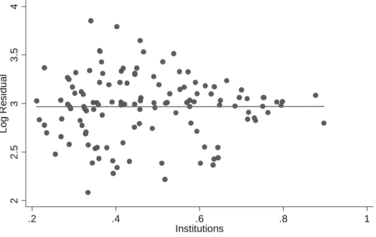
In order to gain further insights into this topic, Chapter III takes Hall and Jones (1999) –one of the earliest contributions to the strand of institutions literature- as a starting point. Using the same data and econometric methodology, we augment their reduced-form regressions so as to include the factors of production, i.e. human and physical capital, and the interactions between institutions and these factors of production. The results are fascinating. First of all, inserting the factors of production into the regression, we notice that the institutions variable –although still significant- loses its magnitude drastically. Secondly, once we allow for the interaction between institutions and the factors of production, the significance of the institutions term vanishes entirely. We call this the moderating effect of institutions (as opposed to a direct effect). Finally, the chapter concludes that by doing the exercise described above, what was called the Solow residual is purged down to a typical random econometric residual.
measures of life satisfaction. This line of research has picked up recently among economists in what is called the economics of happiness.9
Having recognised that the traditional utility and welfare theories have to make a lot of compromises in their assumptions to be able to present a coherent theory, the novelty of the economics of happiness research agenda is to set out by asking the individuals about their perceived life satisfaction (happiness) instead of trying to infer the same information from their consumption patterns. As such, this approach is bound to generate a complementary –perhaps even superior- information on well-being. Possibly, the most noteworthy implication of the discussion above is that although the concept of life satisfaction (happiness) is not necessarily one and the same with the concept of utility, it could be considered as a valid proxy that would yield valuable insights into the topic. By stepping out of the traditional reluctance of the economics profession to attempt to measure utility directly, economics of happiness also opens one of the fundamental areas of economic theory to empirical research.
Having clarified the links of chapter 4 with the economic theory, our aim in this chapter is to provide a systematic analysis of life satisfaction in transition countries, which has not been attempted at this breadth before. Using data from the World Values Surveys, we compare and contrast the experience regarding the correlates of life satisfaction in transition countries with that in the sample of non-transition countries. In other words, we are testing whether the stylised facts that are derived from earlier studies in economics of happiness also hold for the transition countries. Our a priori expectation is to find some differences, given that the transition process from command economy to market capitalism has been a devastating experience for the peoples of these countries. In fact, our findings emphasise that there are indeed several noteworthy differences in the case of the transition countries. First and foremost concerning the individual level correlates of life satisfaction, the most important difference appears to be in the field of self-employment. Accordingly, the self-employed are notably happier in the transition countries, whereas this pattern is reversed in the case of non-transition countries. This is possibly related to the new opportunities of entrepreneurship that the transition process has created.
9
The next step in this chapter is to enrich the analysis by adding macro level variables, such as GDP per capita, inflation, unemployment rate and the Gini coefficient as a measure of inequality, to the econometric specification. Among the results that stand out is the role of inequality. Inequality seems to be particularly disliked in the post-communist societies, which appears not to be the case in the non-transition countries according to the results of our econometric model. A potential explanation for this result is the heritage of the socialist system where equality was one of the most pronounced values.
The role of reforms in the transition process is also a question of interest, especially from a practical policy point of view. This issue is tacked in the relevant section by taking a close look at the reforms as measured by the EBRD transition indicators. Finally, the paper pools the available data from earlier years of the transition period and investigates how happiness has evolved over time for a smaller sample of countries where more than two data points were available. Obviously, the period in question is too short to discern any strong trends in happiness in the sense of time series econometrics, however we were able to detect preliminary evidence in the form of a V-shaped curve, whereby the average levels of perceived happiness dipped in mid-1990s as opposed to the initial years of transition, and as the evidence from late 1990s-early 2000 suggests, they have bounced back, although very few countries report average happiness levels above the values reported in early 1990s. Finally, the chapter concludes by policy recommendations.
These three essays were written separately, yet the common theme to all of them is an emphasis on the institutional setting. The first essay does this in a narrow field of application, namely corruption. The second essay tackles a bigger question, namely the linkages between the institutional environment and growth. Finally, the common thread between these two essays and the last essay in this manuscript is the analysis of the role of reforms in the transition context and relates them to the context of happiness. After all, what better research question can one think of for an aspiring economist, whose ultimate professional goal should be to help foster happiness? On this note, we conclude this section with the words of Jeremy Bentham: “Create all the happiness you can create; remove all the misery you are able to remove.”10
10
PART I
Chapter 2
Between Two Evils:
Grand versus Petty Corruption
2.1 Introduction
It is not uncommon to hear international investors proudly mentioning how corruption functions in their countries of operations facilitating how they conduct their businesses. For instance, under the Suharto regime in Indonesia, investors would just go “top down”, involving a high-ranking Suharto crony and being safe thereafter from any further corrupt requests11. As opposed to this, they also tend to complain that corruption in some other countries is extremely arduous and time consuming. It is this difference that this paper is about. We will recourse both to theoretical reasoning, and empirical tests using the data on FDI and corruption to investigate the validity of such arguments.
It is by now a well established empirical regularity that corruption has negative consequences for the economy. For instance, it asserts an adverse impact on the ratio of investment to GDP, (Mauro 1995 and 1997, Campos, Lien and Pradhan 1999, Brunetti, Kisunko and Weder 1997: 23 and 25; Brunetti and Weder 1998; Gymiah-Brempong 2002). There is equally strong support for the hypothesis that corruption lowers the growth rate of GDP, (Mauro 1997; Tanzi and Davoodi 2001; Leite and
11
Weidmann 1999: 24; Poirson 1998: 16; Pellegrini and Gerlagh 2004; Méon and Sekkat 2003; Gymiah-Brempong 2002). The main channel through which this happens is through lowering capital accumulation; hence it is not surprising that some studies generate insignificant results once investment is controlled for (Mauro 1995; Mo 2001). Among further areas of economic activity where corruption has a significant adverse are productivity (Lambsdorff 2003a), government services and health care, (Gupta, Davoodi and Tiongson 2001) the composition of government expenditures, (Mauro 1998 and 1997; Gupta, Davoodi and Alonso-Terme 2002; Gupta, de Mello and Sharan 2000) and tax revenues (Friedman, Johnson, Kaufmann and Zoido-Lobaton 2000; Tanzi and Davoodi 2001).
The adverse impact of corruption on foreign direct investments (FDI) is also well established. Although Alesina and Weder (1999) report an insignificant relationship, it must be taken into account that first, the authors use data prior to the 1995’s considerable increase in FDI and second, they use a variable by ICRG that measures the political instability due to corruption. This variable depends not only on levels of corruption, but also on the population’s intolerance towards corruption.12 Other papers clearly support the hypothesis that corruption lowers FDI, (Wei 2000a and b, Smarzynska and Wei 2000; Wei and Wu 2001; Habib and Zurawicki 2001 and 2002). Lambsdorff (2003b) shows that overall capital inflows of a country deteriorate due to corruption.
However, the extent to which the impact of various types of corruption may differ has hardly ever been treated empirically so far. Corruption may surface under a variety of guises, such as embezzlement of public funds in public utilities, extortion of speed money in exchange for getting business permits/licences, commissions to parliamentarians to influence the content of the legislation and bribery in public contracts. It is plausible to expect that these actions are likely to have separate consequences.
The only difference in types of corruption that has been the subject of research lately relates to predictability and opportunism. The World Bank (1997: 34) argued: "There are two kinds of corruption. The first is one where you pay the regular price and you get what you want. The second is one where you pay what you have agreed
12
to pay and you go home and lie awake every night worrying whether you will get it or if somebody is going to blackmail you instead." This idea was implemented in a survey by the World Bank and the University of Basel by asking for the predictability of corruption (i.e. absence of opportunism) as well as the overall levels of corruption prevailing in a country. This survey aimed to measure not only whether the costs of corruption are known in advance, but also whether after the (corrupt) payment, the service is delivered as promised. World Bank (1997) investigates the impact of these two variables on the ratio of investment to GDP in a sample of 39 industrial and developing countries. Accordingly, for a given level of corruption, countries with more predictable and less opportunistic corruption enjoy higher investment rates. Further support for this approach is to be found in the work of Campos, Lien and Pradhan (1999), where it is concluded that the nature of corruption also matters in analysing its economic consequences. Lambsdorff (2003b: 237) confirms that besides the levels of corruption, opportunism –defined as to what extent a briber can be confident that the bribee will deliver the promised services once the payment is made- reduces a country’s annual capital inflows.
voluntary decision where investors play an active role in negotiations. This means that they are in better control over the outcome. Section 2.7 presents further tests related to governance indicators and shows that the results of the analysis are robust to their inclusion. Finally, Section 2.8 interprets the results from the point of view of their policy implications, and concludes.
2.2 Theoretical Underpinnings
There are theoretical reasons to expect that international investors are deterred by corruption. Corruption has been shown to inspire cumbersome regulation, and to give incentives to public servants to create artificial bottlenecks. Red tape undoubtedly affects international investors adversely. For instance, Djankov et al. (2000: 47) shows the rates of market entry to fall with increasing levels of corruption.
Akin to a standard adverse selection problem, whereby the wrong type of individuals are selected due to informational asymmetry, e.g. as in the case of people of ill-health buying health insurance, corruption also leads to the selection of the wrong firms, that is, those that are more willing or have better capacity to offer and conceal bribes. In a setting where the advantages from “know-how” would be offset by the absence thereof with respect to “know-who”, investors would definitely be less eager to enter the new market. Furthermore, corruption brings with it the problem of enforcement, which among other things requires trust, (Lambsdorff 2002a). However, it is not necessarily easy for newcomers to instil the same levels of trust as would be readily available at the local level. Further distortions may arise if bribers have the leverage to ask public servants to harass their competitors, (Bardhan 1997: 1322). Local firms are likely to have an edge over their international competitors in arranging such impediments. Due to what may be called ‘local capture’, FDI flows would be distorted towards the home market in case of high levels of corruption. Hence, especially gross FDI inflows would suffer from corruption crowding out international investors. A priori, it is reasonable to expect net FDI inflows to be affected less by corruption because local investors may opt for seizing local (corrupt) opportunities rather than invest abroad. This hypothesis will be tested in sections 2.4 and 2.6.
Noh 1994; Charap and Harm 2000). Once investments are sunk, they become prey to extortion. This comes about mainly because kleptocrats are neither motivated nor constrained to honour their commitments, (Ades and Di Tella 1997: 1026; Mauro 1995). Governments with a reputation for corruption find it difficult to commit to effective policies and to convince investors of their achievements. Corruption therefore deters investors because it goes along with a lacking respect for law, Lambsdorff (2003b).13
So far, we have discussed the potential impact of corruption in a broad perspective. It is yet to be seen, which type of corruption is more detrimental for investors. Corruption may infect a variety of different government functions, all of which may be of different relevance in the eyes of an international investor. Data on corruption in different government functions are available for 1) obtaining export and import permits, 2) getting connected to public utilities (e.g., fixed line telephony, or power grid), 3) annual tax payments, 4) awarding public contracts, 5) dealing with loan applications, 6) influencing the making of laws and policies, regulations, or decrees and 7) influencing judicial decisions. Although this list is far from exhaustive, it captures the essential areas of interface between the public and the private sector.
As will be shown subsequently, corruption in access to public utilities, tax assessments and loan application presents a rather petty type of corruption. In contrast, corruption in public contracts laws and polices and judicial decisions is of a rather grand type. Grand and petty corruption differ in their impact on investors in two major respects.
Arguments related to the organisation of corruption: Petty corruption is
typically defined as the everyday, street-level type of corruption that involves small payments, speed money and tips to relatively low ranking officials. Needless to say, these payments are particularly time consuming, imposing additional costs on investors. For instance, Kaufmann and Wei (1999) document that high levels of corruption are positively associated with the time managers spend with bureaucrats in interpreting rules and regulations. This issue appears particularly relevant for petty
13
corruption.14 Extortion may also be classified as petty corruption. Public office holders may charge additional amounts over and above the official fee for providing certain services. This could be complemented by harassment or further delays unless a payment is made. It might be argued that if corruption is organised as a voluntary arrangement between a briber and a bribee, it might profit the parties involved whilst hampering the third party interests. By contrast, since extortion is beyond the control of the investors and does not entail voluntary engagement, it requires further organizational safeguards and calculations. As such, a country’s reputation for extortion can easily crowd out investment. On the other hand, a reputation for collusion might be lesser of an evil for investors, as it signals credible commitment. Our argument is along the lines of Shleifer and Vishny (1993), who posit that monopolized (grand) corruption should be preferred by investors as opposed to a sequence of requests for petty bribes by decentralized units. While grand corruption would resemble a one-stop-shop, decentralized bribe takers would individually act as monopolists and thus tend to overgraze the market.
Let us take a look at the Shleifer and Vishny argument from a formal theoretical perspective. Consider the objective function of the bureaucrats as a simple profit function in the sense of revenues minus costs. The revenues come from the price they charge for the entitlements. This price should, of course, be an official and transparent fee that covers the bureaucratic costs involved in processing the application in an ideal world. This should be public knowledge and investors should be able to factor this into their cost calculations in advance. Yet, in the world that is not free of corruption, we visualise the revenue of the bureaucrat from this transaction as a percentage of the total amount invested. In other words, the bureaucrat asks t percent of the total investment in order to provide the investor with the required entitlement. She also incurs some costs in this process. The presence of these costs has nothing to do with administrative costs, but it rather stems from the necessity of obfuscating the payments, i.e. concealing the bribe. This is necessary because there is no country in the world, which does not condemn corruption as a
14
criminal activity.15 Assuming that these costs are a positive fraction of the extorted bribes, we can write the cost function as follows:
C =c⋅tiX where 0<c<1
Hence, the profit function of the bureaucrats can be written as revenues minus costs:
, ) 1
( c t X X
ct X
ti − i = − i
=
∏ (2.1)
where X is the amount invested.
Let us also assume that the amount invested is inversely proportional to the amount of the money extorted away from the investor by bureaucrats to deliver the licenses. Let A be the total amount that the investor is prepared to tie to his project. In the absence of bribes, A would be the total amount that he would have invested. Hence, the actual amount invested can be formalised as:
) 1
(
1 = −
= n
i i
t A
X (2.2)
where n is the total number of licences required to start a new investment.
Now, we will consider two broad scenarios. The first one will be the joint profit maximisation of the n departments, which issue the licences. Imagine, for instance, the presence of a strong kleptocrat that dictates the price of the bribes to each department. The second scenario will be one where each department tries to extort the maximum amount in the form of bribes without taking into account the bribes charged by other departments. We will analyse the implications of these two scenarios in terms of the level of investment. The former scenario is that of a top-down type of corruption, and this can easily be mapped into grand type of corruption. Similarly, the latter scenario is one where there is a disorganised competition for bribes. This can be interpreted as a setting where petty corruption prevails.
Scenario 1: Grand Corruption (Joint “Profit” Maximisation of n Departments) Inserting (2.2) into (2.1) yields the following profit function:
15
) 1 ( ) 1 ( 1 = − − = ∏ n i i
iA t
t
c (2.3)
At this stage, we introduce symmetry in the amount of bribes. This comes about because of the presence of a central figure, e.g. a kleptocrat that sets the optimal level of bribes taking into account the joint profit maximisation nature of the problem. Hence, plugging in ti=t in (2.3)
) 1 ( ) 1 ( ] ) 1 ( ) 1 [( nt A t c Ant c A c t − − = ∏ − − − = ∏ ) )( 1
( c t nt2
A − −
=
∏ (2.4)
This is the objective function to be optimised with respect to level of bribes
0 ) 2 1 )( 1 ( − − = = ∂ ∏ ∂ nt c A
t (2.5)
Solving this optimisation problem for t (level of bribes), and calculating the resulting investment and profits leads to an optimal level of bribes in the case of grand corruption at the amount of:
n t
2 1
= (2.6)
which in turn leads to investment and profit levels of:
2 ) 2 1 1 ( ) 1
( X A
n n A nt A
X =
− = − = (2.7) n A c A n c A t c 4 ) 1 ( 2 2 1 ) 1 ( 2 ) 1 ( ∏= − − = − =
∏ (2.8)
Scenario 2: Petty Corruption (Decentralised/Disorganised “Profit” Maximisation of n Departments)
Our starting point is again the objective function defined as equation (2.3). However, a slight modification is necessary in equation (2.2) so as to reflect the change in the nature of the competition for bribes explained above. In this case:
j i
n
i
i t n t
t ( 1)
1
− + = =
in the light of which equation (2.2) could be rearranged as follows:
) ) 1 ( 1
( ti n tj A
X = − − − (2.2’)
What this all means is that in the absence of a central bribe-setter, each department attempts to maximise its own bribe revenue. Therefore, it takes other n-1 departments’ actions into account by including the term tj in its calculations. However, in each department’s calculation this variable is assumed to be independent of ti and is treated as a constant.
The profit function now becomes:
) ) 1 ( 1 ( ) 1
( −c tiA −ti − n− tj
=
∏ (2.3’)
The optimisation process yields the following first order condition: 0 ] ) 1 ( 2 1 [ ) 1 ( − − − − = = ∂ ∏ ∂ j i i t n t A c
t (2.5’)
Given the nature of the problem, we introduce symmetry now. Hence, we plug in t=ti=tj in equation (2.5’). This reflects the fact that the optimisation problem laid out above has been solved n times by n departments and each department arrives at the same optimal level of t.
0 ] ) 1 ( 2 1 [ ) 1 ( − − − − = = ∂ ∏ ∂ t n t A c ti 1 1 0 )] 1 ( 1 [ ) 1 ( + = = + − − = ∂ ∏ ∂ n t n t A c
From equation (2.6’), it follows that: 1 ) 1 1 1 ( ) 1 ( + = + − = − = n A X n n A nt A X (2.7’) 2 ) 1 ( ) 1 ( ) 1 ( ) 1 ( 1 ) 1 ( + − = ∏ + + − = ∏ n A c n A n
c (2.8’)
The results can be summarised in a tabular form as follows:
Table 2.1: Equilibrium by Scenario and Numerical Illustration
Scenario1: Grand Corruption Scenario 2: Petty Corruption
Bribes: t 1/2n 1/(n+1)
Investment: X A/2 A/(n+1)
Profit: ∏ (1-c)A/4n (1-c)A/(n+1)2
Numerical Illustration: c=1/2; A=4800; n=4
Bribes: t 1/8 1/5
Investment: X 2400 960
Profit: ∏ 150 96
It may be argued that this exercise is an oversimplification of the actual phenomenon. However, it serves the purpose of illustrating our point in a relatively simple setting. Evidently, for all n>1, the value of the bribes is lower, moreover total investment and profits are higher in scenario 1, namely grand corruption.16 This gives us a testable hypothesis for the empirical section of the paper: Other things being equal, foreign investors would prefer grand corruption to petty corruption in host countries, where they invest.
Fraudulent opportunities stemming from grand corruption: A cobweb of
investments abroad surrounded with the secrecy of corrupt deals could also generate adverse incentives for investors to boost their own income at the expense of defrauding their firm or their shareholders. Alesina and Weder (1999) argue that corruption may even attract FDI if investors form an ‘inner circle’ to profit from corrupt
16
opportunities. 17 Investment decisions, therefore, may take into account the differences in opportunities generated by grand and petty corruption. Petty corruption tends to be beyond the immediate control of decision makers, whereas the opposite holds true for grand corruption. Winston (1979: 840-1) argues that the risk associated with corruption increases with the number of transactions, the number of people involved, the duration of the transaction and the simplicity and standardization of the procedure. Since the risk does not depend on the value of a transaction, Winston argues that public servants therefore bias their decision in favour of capital intensive, technologically sophisticated and custom-built products and technologies since these generate larger kickbacks. The same logic can be applied to the case of fraudulent investors. Grand corruption provides an efficient base for such fraudulent behaviour. Another reason for investors to be less averse to grand corruption is due to the possibility of exchanging political support in return for enforcing corrupt agreements. For example, during the tenure of former Prime Minister Benazir Bhutto, many private power companies were awarded contracts to sell power to the state Water and Power Development Authority. But the government’s main anti-corruption agency maintained that kickbacks had been paid to bureaucrats and politicians in securing these deals. The new government in place initiated a wholesale renegotiation of the old contracts, cutting the electricity unit price by 30 percent. But, the International Monetary Fund and the World Bank (whose loans to private power companies would sour in case of a price cut) warned the Pakistani government that unilaterally cutting electricity unit rates would seriously lower investor’s confidence. In order to exert pressure on the government, multilateral donors postponed loan agreements.
A related example comes from Indonesia, where, due to charges of corruption, the government's utility authority PLN cancelled its contracts to obtain power from large power plants built by joint ventures with large foreign companies. In this case, relatives of Suharto had been given shares of the operations, raising suspicions of kickbacks and inflated prices for electricity. But foreign delegations of export credit insurers exerted pressure on the Indonesian government to honor the old contracts. It was argued that ”[t]he future investment climate will be shaped by a long-term resolution ... that protects the fundamental rights of investors. ... [Default] will impair
17
Indonesia and our ability to work with you in the future”.18 Such political pressure cannot be organized in the frequent cases of petty corruption, rendering them less attractive.
Corruption in public utilities and loan applications, on the other hand, often involves extortion as there is a clear official service that is demanded. Payments to officials might be made in order to avoid harassment and delay, and in some cases to avoid the official fee. Although there are exceptions to the rule, petty corruption generally necessitates time consuming negotiations over prices, and frequent confrontation with requests as well as additional organizational requirements.
Public contracts, however, are less likely to involve extortion of the type described above. In this type of activity, private firms are free to make their own calculus as to whether to pay bribes or not. Corruption in access to public utilities often happens after investors have incurred sunk costs, whereas corruption in public contracts arises ex ante during the tender, in other words, before investors have committed their resources. At the same time, corruption in areas such as public contracts, laws and policies and judicial decisions tends to be of the grand type. The counterparties deciding on laws, policies and public contracts tend to be higher ranking officials. Investors would be directly involved in the negotiation process and may grab the opportunities to pocket part of the payment.
In sum, two types of corruption are of relevance for our analysis: A petty type of corruption, which is cumbersome to organize, especially in fields such as public utilities and loan applications. The second sort of corruption is the grand, political type related to government policymaking and judicial decisions. The latter is much easier to organize and offers fraudulent opportunities for investors.
18
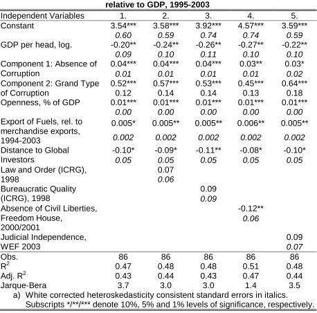
2.3 Data Description
We employ two dependent variables for this study. The first is the gross FDI inflows as a percentage of GDP for the period 1995 to 2003. The annual dollar value of FDI are from the IMF International Financial Statistics, divided by the 2000 GDP in current US dollars from the World Development Indicators database. The second dependent variable is the net FDI inflows as a percentage of GDP for the period 1994 to 2002. The source for this variable is the World Development Indicators 2004.
We delete Luxembourg from the sample of countries since it is an obvious outlier. Theoretically only positive values are possible for gross FDI data. However, if FDI already calculated in previous periods are withdrawn, in some cases negative values may arise. The data on FDI are dealt with in logarithmic form. Due to some observations that are close to or below zero, we add the constant value 0.01 percent of GDP to the gross data prior to taking the logarithm. Similarly, we add one to the net FDI data before taking the logarithm.
Data on subcomponents of corruption for 102 countries in our sample comes from the World Economic Forum’s (WEF) Global Competitiveness Report 2003/04. These variables are constructed as the average responses for each country (of mostly more than 50 business executives per country) from survey questions asking the respondents the following questions:
1. In your industry, how commonly would you estimate that firms make undocumented extra payments or bribes connected with export and import permits? (1 = common, 7 = never occurs)
2. In your industry, how commonly would you estimate that firms make undocumented extra payments or bribes when getting connected to public utilities (e.g., telephone or electricity)? (1 = common, 7 = never occurs)
3. In your industry, how commonly would you estimate that firms make undocumented extra payments or bribes connected with annual tax payments? (1 = common, 7 = never occurs)
4. In your industry, how commonly would you estimate that firms make undocumented extra payments or bribes connected with public contracts (investment projects)? (1 = common, 7 = never occurs)
(1 = common, 7 = never occurs)
6. In your industry, how commonly would you estimate that firms make undocumented extra payments or bribes connected with influencing laws and policies, regulations, or decrees to favour selected business interests? (1 =
common, 7 = never occurs)
7. In your industry, how commonly would you estimate that firms make undocumented extra payments or bribes connected with getting favourable judicial decisions? (1 = common, 7 = never occurs)
We also use further data from the same survey for the absence of Legal Political Donations (WEF 2003; “To what extent do legal contributions to political parties have a direct influence on specific public policy outcomes? 1 = very close link between donations and policy, 7 = little direct influence on policy”), Judicial Independence (WEF 2003; “The judiciary in your country is independent from political influences of members of government, citizens, or firms: 1= No heavily influenced, 7= Yes, entirely dependent), Public Trust in Politicians (WEF 2003 “Public trust in the financial honesty of politicians is 1 = very low, 7 = very high”) and the extent of bureaucratic red tape (WEF 2003 “How much time does your firm’s senior management spend dealing/negotiating with government officials (as a percentage of work time)? 1 = 0%, 2 = 1–10%, 3 = 11–20%, 8 = 81–100%”).
Further explanatory variables used in the study are openness (the sum of imports and exports of goods and services relative to GDP; data from the World Development Indicators, average for 1996-2002), Population (data for 2001 from the World Development Indicators), export of fuels relative to merchandise exports (World Development Indicators, average 1994-2003), growth of GDP (World Development Indicators, average 1990-1995), the share of Protestants (La Porta et al. 1999 and CIA Factbook – where the latter provided only qualitative descriptions a quantitative estimate has been provided by the authors) and distance to global investors (the sum of the distance to Chicago and that to Frankfurt. Data on latitude and longitude are from the CIA Factbook and the distances are calculated according to spherical trigonometry).
provides us with a variable of opportunism in corrupt deals. Further variables of interest employed in this paper are Bureaucratic Quality, and Law and Order from the International Country Risk Guide 1998 and Absence of Civil Liberties from the Freedom in the World publication of the Freedom House. See data appendix for descriptive statistics.
2.4 Data Reduction: Principal Component Analysis
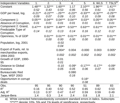
Table 2.2a and b report the results of the regressions to establish the simple link between corruption and FDI. The cross-section regressions model is specified in the following way:
(
)
0 1 2ln FDI GDPi i+0.001 =β β+ Absence corruption_ i+β Xi+εi,
where i is the country subscript. X is a vector of control variables, i is a vector of corresponding coefficients and i is a random error term. We start with a simple
specification where further explanatory variables are disregarded. Accordingly, we only control for GDP per capita to capture the decreasing returns to scale in wealthy countries that drives capital transfers towards developing countries and emerging markets.
Table 2.2.a shows that the absence of corruption in public utilities has the strongest positive impact on FDI, whereas the impact of absence of corruption in law and policies and in judicial decisions is much lower. This initial reduced form evidence is in line with the theoretical arguments presented above.
Table 2.2.a Ordinary Least Squares, a)
Dependent Variable: Average Annual Gross FDI inflows relative to GDP, logged, 1995-2003
Independent Variables
1. 2. 3. 4. 5. 6. 7
2.94*** 3.58*** 3.33*** 2.90*** 2.85*** 2.74*** 2.74*** Constant
0.55 0.60 0.59 0.56 0.57 0.55 0.55
-0.01 -0.20* -0.11 0.03 -0.02 0.06 0.08 GDP per head, log.
0.08 0.10 0.09 0.08 0.09 0.07 0.07
0.17** Absence of
Corruption, Export and Import
0.07
0.35*** Absence of
Corruption, Public Utilities
0.09
0.26*** Absence of
Corruption, Tax Payments
0.08
0.11* Absence of
Corruption, Public Contracts
0.07
0.19** Absence of
Corruption, Loan Applications
0.08
0.091 Absence of
Corruption, Laws and Policies
0.06
0.04 Absence of
Corruption, Judicial Decisions
0.05
Obs. 95 95 95 95 95 95 95
R2 0.09 0.19 0.15 0.07 0.09 0.06 0.05
Adj. R2 0.07 0.17 0.13 0.05 0.07 0.04 0.03
Jarque-Berab) 0.7 1.3 0.9 0.9 1.3 0.7 0.7
a) White corrected heteroskedasticity consistent standard errors in italics.
Subscripts */**/*** denote 10%, 5% and 1% levels of significance, respectively.
Table 2.2.b Ordinary Least Squares, a)
Dependent Variable: Average Annual Net FDI inflows relative to GDP, logged, 1995-2002
Independent Variables 1. 2. 3. 4. 5. 6. 7
1.00** 1.79*** 1.53** 0.92* 1.00* 0.77 0.77 Constant
0.50 0.51 0.50 0.53 0.54 0.50 0.52
-0.05 -0.26*** -0.18** -0.005 -0.08 0.02 0.04 GDP per head, log.
0.07 0.08 0.07 0.09 0.07 0.07
0.16** Absence of
Corruption, Export and Import 0.07 0.36*** Absence of Corruption, Public Utilities 0.08 0.28*** Absence of Corruption, Tax Payments 0.07 0.11 Absence of Corruption, Public Contracts 0.07 0.21** Absence of Corruption, Loan Applications 0.08 0.09 Absence of
Corruption, Laws and Policies 0.07 0.05 Absence of Corruption, Judicial Decisions 0.06
Obs. 95 95 95 95 95 95 95
R2 0.06 0.17 0.13 0.05 0.07 0.04 0.03
Adj. R2 0.04 0.15 0.11 0.02 0.05 0.02 0.01
Jarque-Berab) 0.5 2.2 0.8 0.5 0.7 0.5 0.3
c) White corrected heteroskedasticity consistent standard errors in italics. Subscripts */**/*** denote 10%, 5% and 1% levels of significance, respectively.
d) The Jarque-Bera measures whether a series is normally distributed by considering its skewness and kurtosis. The assumption of a normal distribution can be clearly rejected for levels above 6
Although the second component has an Eigenvalue clearly below the Kaiser criterion of 1, we believe it represents valuable information and is not just noise. First, the overall perceived level of corruption comes out quite strongly in the results mainly due to the similar phrasing of all questions. Had questions been asked for differences in types of corruption, the second component would most likely to obtain a higher Eigenvalue.19 Second, this analysis is replicable for both 2002 or the 2004 data by the WEF, that is, the second factor derived here is qualitatively similar across these years, emphasising the robustness of the findings.
Table2.4 presents the coefficients for the two components.
The interpretation of the first component as the overall absence of corruption is a straightforward matter, especially given that all the factor loadings have the same sign. Component 2 is orthogonal to the first component and relates to the particular
19
In this respect the Kaiser criterion is not invariant to matrix operations, such as substituting corruption in public utilities by the difference of this type of corruption to that in government programs.
Table 2.3: Total Variance Explained, Data on Corruption by the WEF 2003
Initial Eigenvalues
Total % of Variance Cumulative %
Component 1 6.333 90.464 90.464
Component 2 0.325 4.640 95.105
Table 2.4: Coefficient Matrix, Data on Corruption by the WEF 2003
Extraction method: Principal Component Analysis
Component 1 Component 2
Absence of Corruption, Export and Import .972 .059 Absence of Corruption, Public Utilities .930 .306
Absence of Corruption, Tax Payments .965 .100
type of corruption. On the one hand, corruption in public contracts, government policymaking and judicial decisions share the same negative sign for component 2. On the other hand, corruption in exports and imports, public utilities, tax payments and loan applications share a positive sign. The strongest difference in factor loadings is observed between corruption in government policymaking and corruption in public utilities.
High values of the component 2 indicate the prevalence of corruption in laws and policies, in judicial decisions and public contracts. It is plausible to think of these as forms of grand corruption. By contrast, low values of the component 2 point at the prevalence of corruption in public utilities and loan applications (and to a lesser extent in tax payments and in obtaining export and import permits). Hence lower values of this component capture petty corruption which necessitates cumbersome organizational efforts.
To illustrate how this component functions, let us think of a hypothetical situation where grand corruption is rampant and there is almost no petty corruption. The original corruption variable from the survey assigns the value 1 to cases where corruption is common and 7 to those where it never occurs. Hence, in the case of grand corruption, absence of corruption in public contracts, laws and policies and judicial decisions will all receive low values from respondents, say 1, and the rest will get high values indicating that corruption never occurs in these fields, say 7. Then, the second component will yield:
Component 2 = (.059*7)+(.306*7)+(.100*7)+(-.146*1)+(.223*7)+(-.273*1) + (-.269*1) =4.128
Similarly, in the opposite situation whereby petty corruption is rampant and there is no grand corruption, the same component will yield:
Component 2 = (.059*1)+(.306*1)+(.100*1)+(-.146*7)+(.223*1)+(-.273*7) + (-.269*7) = -4.128
interpreted as the relative importance of grand corruption as opposed to petty corruption. It must be said, however, that this variable is related exclusively to the relative importance of grand versus petty corruption, and disregards the levels of corruption. Hence, in the subsequent regression analysis, we will control for the absolute level of corruption with the component 1, and the relative importance of the type of corruption using component 2.
Besides making a novel interpretation of the data possible, another sizeable benefit derived from this data reduction exercise is that by imposing orthogonality condition on the components, we get rid of the multicollinearity problem, which would otherwise cast doubt on the validity of our estimates in our subsequent regressions.
2.5 Analysis of the Components
In order to better understand what these components imply, we run a series of OLS regressions in Table 2.5. Accordingly, respondents of the World Economic Forum survey perceive South America, Central America and the Caribbean and Eastern Europe including countries of the Former Soviet Union to fall prey to grand corruption. Particular examples to be mentioned here are Argentina, Bolivia, Ecuador, El Salvador, Guatemala, Nicaragua, Peru, Philippines, Slovak Republic and Venezuela. On the other hand, petty corruption is perceived to prevail in Africa. The countries with the lowest values for component 2 are Bangladesh, Cameroon, Egypt, Gambia, Ghana, Morocco, Tunisia and Zambia.
Columns 3-5 present further evidence in favour of our interpretation that component 2 is measures the type of corruption. Using further variables from the same data source, column 3 shows that component 2 decreases with public trust in politicians, with the absence of legal political donations to influence public decisions and with bureaucratic red tape. The negative sign supports our interpretation because the case of grand corruption would be associated with legal political donations, involve little trust in politicians and not depend on bureaucratic red tape.
Table 2.5. OLS, a)
Dependent Variable: Component 2: Type of Corruption
Independent Variables 1. 2. 3. 4. 5.
0.36*** 0.30 1.21** 0.15 1.24
Constant
0.04 0.35 0.47 0.29 0.75
-0.006 0.04 0.10*** -0.02 GDP per head, log.
0.03 0.03 0.04 0.09
-0.19*** -0.18* -0.15* Dummy variable, Africa
0.06 0.10 0.09
0.27*** 0.30*** 0.10 Dummy variable, Eastern
Europe and Former Soviet Union
0.08 0.09 0.08
0.69*** 0.70*** 0.44*** Dummy variable, South
America 0.12 0.12 0.12
0.44*** 0.45*** 0.20 Dummy variable, Central
America and Caribbean 0.11 0.12 0.12
-0.07 -0.07 -0.050 Dummy variable,
Asia 0.10 0.10 0.08
-0.18*** -0.20** Opportunism in corrupt deals
0.06 0.08
0.65 Grand – petty corruption
0.43 -0.10**
Absence of Legal Political
Donations, WEF 2003 0.05
-0.08** Public Trust in Politicians,
WEF 2003 0.04
-0.20** Bureaucratic Red Tape,
WEF 2003 0.08
Obs. 101 99 99 55 31
R2 0.51 0.52 0.64 0.11 0.17
a) White corrected heteroskedasticity consistent standard errors in italics. Subscripts */**/*** denote 10%, 5% and 1% levels of significance, respectively.
corruption. Nevertheless, this index obtains the expected sign supporting our interpretation, although it fails to reach conventional levels of significance possibly due to the restricted sample.
2.6 The Type of Corruption and FDI
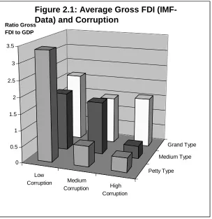
Figure 2.1 presents in three-dimensional space the average gross FDI inflows relative to GDP , the overall level of corruption (component 1), and the type of corruption (component 2). As expected, when the level of corruption is low, its type is of little relevance for FDI. However, in the case of high corruption, grand corruption might be more desirable than petty corruption as it is associated with higher levels of FDI.
Figure 2.2 presents exactly the same exercise for the case of the net FDI inflows figures. The insights from this figure are also similar. In fact, the punch line from the first figure, i.e. that in high levels of corruption there is a clear tendency that grand corruption as opposed to middle and low-level corruption supports FDI, where the type loses relevance, becomes even stronger.
Low
Corruption Medium
Corruption High Corruption
Petty Type Medium Type
Grand Type
0 0.5 1 1.5 2 2.5 3 3.5 FDI to GDP
Figure 2.1: Average Gross FDI (IMF-Data) and Corruption
After presenting this visual evidence, we now incorporated the two components into the regressions on gross FDI in Table 2.6.a. Our strategy to set up the regressions is inspired by the approach of Habib and Zurawicki (2001 and 2002). The regressions are set up parsimoniously in order to focus on the impact of the two components on FDI. Both components are significantly, as shown in column 1. By construction, absence of corruption (component 1) ranges between 15 and 45 with a standard deviation of 7.5. Based on this column, a one-standard deviation increase in the absence of corruption increases the logarithm of the ratio of gross FDI to GDP by 0.33. In other words, it increases gross FDI by one third. Component 2 has a standard deviation of 0.4. Increasing component 2 (grand corruption as opposed to petty corruption) by one standard deviation20, leads to a surge in the logarithm of the ratio of gross FDI to GDP by 0.3, which corresponds to an increase of roughly 35%.
These basic results remain unaffected by the inclusion of further control variables. On the basis of Mauro (1995) results indicating that corruption’s impact on growth materialises through the channel of investment, we included two potential variables that emanate from growth theory, namely the domestic savings rate and the
20
For example, by decreasing absence of corruption in public utilities by 1.3 (on a scale from 1 to 7) or by increasing absence of corruption in government programs by 1.4 (on a scale from 1 to 7).
Low
Corruption Medium
Corruption High Corruption
Petty Type Medium Type
Grand Type
0.5 0.7 0.9 1.1 1.3 1.5 1.7 Ratio Net FDI to GDP
population growth rate. Using data from the World Development Indicators, we tested, these variables, yet they were insignificant without affecting other coefficients. Hence, the results are not reported in the table. A country’s level of integration to the world economy is one of the important factors to explain the FDI it receives. This can be proxied by openness, the sum of import and exports relative to GDP. This variable obtains the expected positive impact (column 2, Table 2.6.a).21
FDI statistics tend to be biased towards smaller countries. This is because in larger countries, sizeable investment flows take place within the borders, and as such are not recorded as FDI. For instance, investments originating from California to New York are not classified as FDI, whereas those from Portugal to Spain are. To account for this bias we control for the (logarithm of) population. This variable obtains the expected sign, yet missing conventional levels of significance, (column 3, Table 2.6.a). Given that the same result is also replicated in other specifications, we exclude this variable from subsequent regressions.
It is often argued that resource rich countries attract more FDI simply because of higher returns to investment. To proxy for this, we include a variable on the export of fuels relative to merchandise exports. Indeed, the variable is significant and carries the expected sign. In order to control for the possibility that the FDI we observe in our period of interest might be motivated by high growth rates preceding the period of investment decision, we control for the average GDP growth between 1990 and 1995. Yet, the variable is insignificant, as shown in column 3.
The location of a country is expected to play a key role in investment decisions. The distance to major markets is especially crucial if the foreign investors aim to use the host country as an export base. We expect that the more distant is a country to the USA and Western Europe, the less likely it is to attract incoming FDI. We use spherical trigonometry to calculate the distance to major markets, in our case, the distance to Chicago, USA and to Frankfurt am Main, Germany. Accordingly, the data on distance can take on a maximum value of =3.14 for distance to one major market. Given that we are adding up the distance to Chicago and that to Frankfurt, the values are bounded to be below 2 . The highest value in this calculation was obtained by New Zealand with 5.0. Other South East Asian countries as well as
21