† Corresponding author
DOI: 10.18488/journal.aefr/2015.5.4/102.4.693.708
ISSN(e): 2222-6737/ISSN(p): 2305-2147
© 2015 AESS Publications. All Rights Reserved. 693
FINANCIAL
CRISIS
AND
FINANCIALIZATION
ACUITY
ON
THE
DIVERSIFICATION BENEFITS OF COMMODITIES: A STOCHASTIC ASSET
ALLOCATION FRAMEWORK
Velappan Shalini
1†--- Krishna Prasanna P
21
Doctoral Scholar, Department of Management Studies Indian Institute of Technology Madras Adayar, Chennai, Tamil
Nadu India
2Associate Professor, Department of Management Studies Indian Institute of Technology Madras Adayar, Chennai, Tamil
Nadu India
ABSTRACT
This research investigates the portfolio diversification benefits of commodities in the backdrop of
uncertainty caused by the financial crisis, increased Financialization and speculation in
commodity markets. Portfolios are formed out of varied asset classes comprise of equity, bond,
infra structure, commodity spot & futures indices and sectoral indices such as agri, metals and
energy sectors over a period 2005-2013. It employed stochastic mean-conditional value at risk
(CVaR) optimization model. CVaR quantifies downside risk and helps to minimize extreme losses.
The ex-post stability of the results and the robustness of the model are validated through back
testing. Different performance measures such as Sharpe ratio, modified Sharpe ratio with
conditional value at risk, opportunity cost and maximum draw down are employed to compare the
results of multi asset portfolios. The results support the evidence of the diversification benefit in
commodity futures indices than in spot indices. It also highlighted the significance of Agri
commodities in offering portfolio diversification than energy and metal commodities. The
diversification benefit of later are found to be reduced with the advent of financial crisis. It also
provides empirical evidence that the diversification benefits of energy and metal commodities were
reduced during the financial crisis and this can be attributed to the observed increase in
Financialization and cross-asset market integration during the crisis period.
© 2015 AESS Publications. All Rights Reserved.
Keywords
:
Commodity spot and futures indices, Energy, Metal and agri, Diversification benefits, Financial crisis,Financialization, Conditional value at risk portfolio optimization, India.
Asian Economic and Financial Review
ISSN(e): 2222-6737/ISSN(p): 2305-2147© 2015 AESS Publications. All Rights Reserved. 694
JEL Classification:
G01, G11, C61.Contribution/ Originality
This study uses new estimation methodology to evaluate the diversification benefit of commodity by addressing the uncertainty in the asset returns, the time varying nature of
correlation-covariance structure and extreme distribution losses, by modelling through scenario based Mean - CVaR (Conditional Value at Risk) stochastic optimization.
1. INTRODUCTION
With the advent and growth of alternative investment houses such as pension funds, hedge funds and exchange traded funds, the evaluation of portfolio diversification benefits has caught the
attention of contemporary researchers. Commodities serve as an effective inflation hedge and offer diversification benefits because of low or negative correlation with conventional assets like stocks and bonds. This key idea was challenged by the recent evidence of cross market co-integration and
an increased correlation across asset markets followed by financialization and the financial crisis (Nissanke, 2012; Silvennoinen and Thorp, 2013). Hence, this paper studies the diversification
benefits of commodities in an asset allocation framework.
Recent literature documented the diversification benefits and proposed that including
commodities in a portfolio of conventional assets leads to enhanced return and risk trade-off and better portfolio performance (Jensen et al., 2002). Moreover the diversification benefits of commodities were arguably limited to upswings in the commodity markets. He also found that the property of low and negative correlation did not hedge the risk of equity markets during a bearish
phase. Daskalaki and Skiadopoulos (2011) argued against the diversification benefits of including commodities in a portfolio.
While research studies in commodity markets that have examined diversification benefits
using portfolio theory are limited (Chong and Miffre, 2010), these studies have also focused only on a single commodity index, which leads to biased results as commodities possess a high degree
of heterogeneity which a single index fails to capture (Erb and Harvey, 2006). Further, asset allocations were made in a static mean variance framework (Daskalaki and Skiadopoulos, 2011).
You and Daigler (2013) observed volatile risk and return characteristics in the ex-ante and ex-post portfolio performance and reported that these are caused by time varying returns. The recent
environment of uncertainty caused by the financial crisis emphasizes the need to devise and employ methods that circumvent the extreme fluctuations in the asset returns distribution.
This study adds to the previous body of work and analyzes the diversification benefits using stochastic asset allocation setting focusing on downside risks and extreme losses rather than use a
static Markowitz mean-variance framework (Markowitz, 1952). Since commodity markets are heterogeneous, the diversification benefits of multiple sectors such as energy, metals and agriculture have been investigated in the present study rather than analyzing only a single
© 2015 AESS Publications. All Rights Reserved. 695 The novelty of this study is that it analyzes the diversification benefits of commodities by taking into account the uncertainty in the asset returns, the time varying nature of
correlation-covariance structure and extreme distribution losses, by modelling through scenario based Mean - CVaR (Conditional Value at Risk) stochastic optimization. In addition, sectoral indices, both spot and futures, for energy, metals and agriculture were used as the means by which investors can
access commodity asset classes. The out of sample performance and stability of the results was assessed by rolling estimation of Mean - CVaR portfolio optimization and back-testing. The
performance of the portfolios augmented with commodities and the portfolios with only conventional asset classes were examined by different performance measures. These measures
include the conventional Sharpe ratio, the modified Sharpe ratio with CVaR and draw down at risk. An opportunity cost based on the incremental performance of the commodity portfolio with the
conventional portfolio has also been examined over the time periods to provide better insights into the relative outperformance with respect to changing market dynamics.
The rest of this paper is organized as follows: Section 2 describes the data; Section 3 describes
the methodology; the results are discussed in Section 4 and Section 5 concludes the paper.
2. DATA
The Indian commodity exchange, named the Multi Commodity Exchange (MCX), was started
in 2003, but historical trade data is available only since July 2005.The data period for this research spans from July 2005-December 2013, which includes both the bullish and the bearish periods. The
sample period covers the 2008 financial crisis; the 2010 sovereign debt crisis, and also the commodity boom periods and increased Financialization times. Thus, the data facilitates the
examination of the effect of all these important events in a commodity asset allocation decision. The data includes the spot index of the Multi Commodity Exchange referred as MCXS Comdex and its sub-indices, MCXS Energy, MCXS Metal and MCXS Agri. The futures indices of the Multi
Commodity Exchange (MCX) such as MCX Comdex and its sub-indices, MCX Energy, MCX Metal and MCX Agri were also included for this analysis. The above data was sourced from the MCX, which is India’s largest and one of the world’s prominent commodity exchanges.
Conventional equity investments have been represented by monthly returns from CNX Nifty
50, which is a benchmark index of the National Stock Exchange. CNX Infra index was included to proxy infrastructure asset movements. The T-bill index of Clearing Corporation of India Limited
(CCIL) represents the impact of bond market investments.
Descriptive statistics of the data are given in Table 1 and the results of correlation matrix are
given in Table 2. CNX Nifty 50 index as well as MCX -Metal were found to be assets with higher returns. However, the volatility of equity returns was observed to be higher than that of metals.
Median value of all the assets was higher than the mean values, indicating that actual returns were higher than the mean value across the sample periods. Further, negative skewness in the asset returns indicated higher negative returns compared to positive returns. The infra index had highest
© 2015 AESS Publications. All Rights Reserved. 696 The correlation matrix (Table 2) proves the diversification benefits of adding different asset
classes to portfolio in order to minimize the systematic risk related to a specific market. Assets with
either negative or lower correlation provide the desired diversification benefits. Only T-bill returns representing bond investments had a negative correlation with all the assets. Equity index had a significant positive correlation with all the commodity indices except with metals and agri indices.
While metals had a negative significant correlation, agri spot and futures indices had lower insignificant positive correlation. Infrastructure index had a low positive or negative correlation
with all the assets except Nifty 50. This indicates that a combination of Nifty, metals, agri and T-bill would optimize diversification benefits.
Table-1. Descriptive statistics of sample assets
Notes: This table shows the descriptive statistics of average monthly log return of various asset classes such as Comdex futures, Energy futures, Metal futures, Agri futures, Comdex spot, Energy spot, Metal spot, Agri spot, Mibor, T-Bill, Nifty 50 and Infra indices. Study period is from July 2005 to December 2013.
Table-2. Correlation matrix across the assets
Notes: This table shows the correlation matrix of average monthly log return of various asset classes such as Comdex futures, Energy futures, Metal futures, Agri futures, Comdex spot, Energy spot, Metal spot, Agri spot, Mibor, T-Bill, CNX Nifty 50 and CNX Infra indices. Study period ranges from 2005 July to 2013 December. ** and * indicates that correlation is significant at 0.01and 0.05 confidence level.
3. METHODOLOGY
In this research study Mean-CVaR portfolio optimization has been deployed to evaluate the
© 2015 AESS Publications. All Rights Reserved. 697 1997). CVaR maximizes the conditional expected portfolio returns below a pre-specified low percentile of the distribution and minimizes anticipated losses in turbulent market times.
Let I={1,2,3,....,n} be the investment asset sets and the rate of returns for each individual asset
i is represented by a random vector r= (r1,....,rn).The decision variable defining the portfolio proportion of different financial instruments is represented by the decision vector x=(x1,....,xn). The
returns of each portfolio x is the sum of individual instruments in the portfolio, scaled by its proportions xj. The expected returns on portfolio is given by
∑
The mean rate of return for the portfolio x is given by
∑
Considering J scenarios with probabilities θj, where j=1,....,J assumption is made that for each
random variable its realization under scenario j is known. The probability of scenario
generation J historical periods as equally probable scenarios and θj =1/J, j=1,...,J, then the
realization of portfolio returns, is given by
∑
∑
∑
equals to
∑
Objective function:
∑
subject to
(7)
∑
© 2015 AESS Publications. All Rights Reserved. 698 where, , returns of the asset is random and is the return of i-th scenario j, j=1,....,J. The vector
of asset returns y= r= (r1,....,rn) is random. The risk constraint , in optimization problem equation (9) for a specified probability level can be read as
∑ ( ) ∑
where, f(x,y) is the loss function for each x and induced by y is a random variable and measures the corresponding VaR for a specified .
For each monthly observation T in the data set, the rolling window K was used in the portfolio weight calculations, where K T. The weights of asset allocation were estimated by minimizing
the CVaR at any given point t, t T from previous K observations. The out-of-sample realized return over the period [t, t+1] was observed from the estimated weights at time t. This process was repeated until the end of the sample period by excluding the earliest one and integrating the next
period return. This study has 96 monthly observations, T= 96 rolled over a window of size K=24. Three alternative measures such as Sharpe ratio (Sharpe, 1964), opportunity cost Simaan (1993)
and conditional drawdown Krokhmal et al. (2002) at risk were employed to compare the performance of the resulting Mean- CVaR optimal portfolios with and without commodities.
4. RESULTS AND DISCUSSIONS
This section discusses the out-of-sample results obtained from the Mean-CVaR optimized portfolios constructed with both conventional assets and commodities. Tables 3 and 4 present the
results of the Mean-CVaR portfolio optimization for different rolling windows. A conventional portfolio comprises of Nifty 50, T-Bill and CNX Infra indices. The commodity portfolio was augmented with additional commodities indices and sub-indices, both spot and futures
independently. Alternative performance measures such as the Sharpe ratio, the modified Sharpe ratio, conditional drawdown at risk, and opportunity cost for the respective rolling window
estimation are given in these tables.
Table-3. Commodity diversification benefits with MCX Comdex spot
Portfolio performance measures
Rolling Window 12 Rolling Window 18 Rolling Window 24
Conventional Asset class Expanded Asset class Conventional Asset class Expanded Asset class Conventional Asset class Expanded Asset class Sharpe ratio(SR)
SR_SD 2.17 1.05 2.20 2.09 2.13 2.02
SR_CVaR 11.96 11.39 20.98 19.01 32.25 10.26
CDaR
Minimum 0.0015 0.0012 0.0030 0.0030 0.0030 0.0022 1st quad 0.0027 0.0023 0.0032 0.0030 0.0032 0.0034 Median 0.0038 0.0023 0.0035 0.0030 0.0035 0.0045
© 2015 AESS Publications. All Rights Reserved. 699
Mean 0.0035 0.0026 0.0035 0.0034 0.0035 0.0040
3rd quad 0.0045 0.0035 0.0037 0.0037 0.0037 0.0050 Maximum 0.0053 0.0037 0.0039 0.0043 0.0040 0.0054 Opportunity
returns/losses
Minimum -0.0239 -0.0265 -0.0165
1st quad -0.0062 -0.0178 -0.0051
Median 0.0000 -0.0134 -0.0011
Mean 0.0019 -0.0111 -0.0022
3rd quad 0.0128 -0.0039 0.0000
Maximum 0.0392 0.0024 0.0071
Notes: This table reports the performance measures such as Sharpe ratio, conditional drawdown at risk (CDaR) and opportunity returns/losses of Mean-CVaR optimized portfolio with conventional assets-Nifty 50 and Tbill and portfolio augmented with Comdex spot indices and sub-indices namely, MCXS Comdex, MCXS Energy, MCXS Metal and MCXS Agri. Monthly observation are used in out of sample back-testing approach of Mean-CVaR optimization for three different rolling windows of sample size, 12, 18, 24.
Commodity spot for a rolling window 12 Commodity spot for a rolling window 18
Commodity spot for a rolling window 24
Graph-1. Relative out-performance of portfolio with commodity spot Vs conventional asset class
Notes: This graph indicates the excess returns or losses of an optimal portfolio formed in the Mean-CVaR framework with and without commodities. The returns/losses are calculated from the opportunity investment cost given in equation (14). The percentage of relative loss is given in the x-axis and the time period is given in the y-axis. The positive percentage indicates that the Mean-CVaR optimal portfolio with commodities outperformed the Mean-CVaR optimal portfolio without commodities and vice-versa.
© 2015 AESS Publications. All Rights Reserved. 700 MCXS Metal and MCXS Agri) and the relative out-performance is given in Graph1. The
augmented portfolio returns represented by the Sharpe ratio were not higher than
conventional portfolios.
Both the portfolios appeared to offer similar returns. However, commodity portfolio risk was lower for a rolling window of 12 and 18 months. This indicates that the inclusion of
commodity spot provides diversification, by marginally reducing risk rather than increasing returns.
On comparison of opportunity returns and losses, a 12 month rolling window offered a better performance. Graph 1 presents the excess returns or losses of an optimal portfolio
formed in the Mean-CVaR framework with and without commodities.
The positive percentage indicates that the Mean-CVaR optimal portfolio with
commodities outperformed the Mean-CVaR optimal portfolio without commodities and vice-versa. This graph also supports the fact that portfolios with commodities rebalanced with an investment window of 12 months and provided relatively better results.
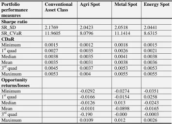
Table 3.1 presents the diversification benefits of including each of the three commodities - agri, metal and energy assets for a rolling window of 12 months.
Table-3.1. Diversification benefits individual commodity spot
Portfolio performance measures
Conventional Asset Class
Agri Spot Metal Spot Energy Spot
Sharpe ratio
SR_SD 2.1769 2.0423 2.0518 2.0441
SR_CVaR 11.9605 8.0796 11.1414 8.6315
CDaR
Minimum 0.0015 0.0012 0.0018 0.0015
1st quad 0.0027 0.0035 0.0026 0.0021
Median 0.0038 0.0035 0.0041 0.0038
Mean 0.0035 0.0031 0.0038 0.0036
3rd quad 0.0045 0.0037 0.0053 0.0053
Maximum 0.0053 0.004 0.0055 0.0055
Opportunity returns/losses
Minimum -0.0292 -0.0274 -0.0351
1st quad -0.0166 -0.0154 0.0258
Median -0.0126 0.013 -0.0243
Mean -0.0101 -0.0898 -0.0165
3rd quad -0.190 -0.000 -0.0003
Maximum 0.0109 0.012 0.0026
© 2015 AESS Publications. All Rights Reserved. 701 Commodity metal spot for a rolling window 12 Commodity energy spot for a rolling window 12
Commodity agri spot for a rolling window 12
Graph-2. Relative out-performance of portfolio with individual commodity spot Vs conventional asset class Notes: This graph indicates the excess returns or losses of an optimal portfolio formed in the Mean-CVaR framework with and without commodities. The returns/losses are calculated from the opportunity investment cost given in equation (14). The percentage of relative loss is given in the x-axis and the time period is given in the y-axis. The positive percentage indicates that the Mean-CVaR optimal portfolio with commodities outperformed the Mean-CVaR optimal portfolio without commodities and vice-versa.
The risk return profile of portfolios presented in Table 3.1 explains that individual commodity
sectors do not offer higher returns as compared to conventional portfolios and the relative out-performance is given in Graph 2. Agriculture commodities offer lower risk and a combination of
agri and metals spot offers a moderate risk return profile.
Table 4 presents the Mean-CVaR optimized weightage of conventional portfolios. The
conventional asset portfolios were made out of bond, equity and infrastructure indices. Since a Mean-CVaR optimization model minimizes the downside risk for risk-averse investors, bonds had
higher weightages than equity markets in the conventional portfolio. The infrastructure index had asset allocation only in 2009. The weights reported here were for a rolling window of 12. The first portfolio was formed in July 2006 and the same year had 6 portfolios, while the rest of the years
had 12 portfolios every year. The weightages of monthly portfolios are averaged yearly and the results are presented in this table for brevity.
Table 5 presents the Mean-CVaR optimized weightages of portfolios augmented with 7 different spot commodities. The iterative weightages allotted to each asset are given for each model
in the table. These portfolios comprised of bond, equity, and infrastructures indices along with their respective commodity indices. Each model represents a different combination of assets for
© 2015 AESS Publications. All Rights Reserved. 702 It was found that the agri index had higher weightage followed by metal and energy spot respectively. It is noteworthy that commodities were given allocation by the optimizer only after
the 2008 financial crisis period.
The MCXS Comdex spot received minimal weightage when all sectoral indices were added. This indicates that commodities possess heterogeneity and adding a single commodity is not
beneficial when compared to adding multiple assets. The results of Table 5 further highlights the continuous allocation of agri spot from 2007-2014. Energy spot also received allocation but its
weightage was low when compared to agri and metal spots. Metal spot was found to have allocated only during 2008-2011.
Table-4. Portfolio Compositions: Conventional Asset class
Assets/Year 2006 2007 2008 2009 2010 2011 2012 2013
Bond 0.71 0.74 0.757 0.784 0.778 0.787 0.755 0.699
Equity 0.29 0.26 0.24 0.20 0.22 0.21 0.24 0.3
Infrastructure 0.014 0.003 0.001
Notes: The weights of respective Mean-CVaR optimized portfolios of conventional assets are presented in this table. The monthly weights are averaged to get yearly portfolio weights for better understanding.
Table-5. Portfolio Compositions: Commodity spot and their combinations Model 1: MCX Comdex spot
Assets/Year 2006 2007 2008 2009 2010 2011 2012 2013
Bond 0.710 0.788 0.729 0.716 0.686 0.730 0.765 0.695
Equity 0.290 0.21 0.26 0.25 0.3 0.24 0.22 0.29
Infrastructure 0.001 0.014 0.003 0.001 0.002
COMDEX spot 0.001 0.002 0.001
Agri spot 0.001 0.002 0.015 0.010 0.012 0.006 0.002
Metal spot 0.004 0.002 0.003 0.007 0.002
Energy spot 0.003 0.006 0.003 0.009
Model-2. Agri Spot
Assets/Year 2006 2007 2008 2009 2010 2011 2012 2013
Bond 0.71 0.729 0.689 0.726 0.757 0.774 0.728 0.779
Equity 0.29 0.27 0.3 0.24 0.23 0.2 0.26 0.21
Infrastructure 0.001 0.014 0.003 0.001 0.001
COMDEX spot 0.007 0.003 0.013 0.003 0.008
Agri spot 0.001 0.003 0.016 0.011 0.010 0.004 0.002
Model-3. Metal Spot
Assets/Year 2006 2007 2008 2009 2010 2011 2012 2013
Bond 0.78 0.75 0.769 0.711 0.704 0.735 0.702 0.79
Equity 0.22 0.25 0.22 0.27 0.29 0.25 0.29 0.2
Infrastructure 0.001 0.015 0.003 0.001 0.001
COMDEX spot
0.003 0.002 0.007 0.003 0.009
© 2015 AESS Publications. All Rights Reserved. 703 Model-4. Energy Spot
Assets/Year 2006 2007 2008 2009 2010 2011 2012 2013
Bond 0.7 0.7 0.691 0.781 0.798 0.783 0.742 0.726
Equity 0.3 0.3 0.3 0.2 0.2 0.2 0.25 0.26
Infrastructure 0.001 0.015 0.003 0.001 0.002
COMDEX spot
0.006 0.003 0.012 0.001 0.005
Energy spot 0.002 0.002 0.002 0.007
Notes: The weights of respective Mean-CVaR optimized portfolios of conventional assets with commodity spot in different iterations are presented in this table. The monthly weights are averaged to get yearly portfolio weights for better understanding.
The impact of the inclusion of commodity futures together with conventional assets was
investigated and Table 6 presents the results of portfolios which included four commodity indices (MCX Comdex, MCX Energy, MCX Metal and MCX Agri).
Table-6. Commodity diversification benefits with MCX Comdex futures
Portfolio Rolling Window 12 Rolling Window 18 Rolling Window 24
performance
Conventional Expanded Conventional Expanded Conventional Expanded
Conventional Asset class Expanded Asset class Conventional Asset class Expanded Asset class Conventional Asset class Expanded Asset class measures
Asset class Asset class Asset class
Asset
class Asset class
Asset class Sharpe
ratio 2.08 2.17 2.20 2.21 2.11 2.13
SR_SD 5.44 11.96 20.98 24.54 7.07 32.25
SR_CVaR
CDaR 0.0015 0.0015 0.0030 0.0006 0.0030 0.0005
Minimum 0.0027 0.0018 0.0032 0.0007 0.0032 0.0026 1st quad 0.0038 0.0020 0.0035 0.0012 0.0035 0.0048 Median 0.0035 0.0048 0.0035 0.0016 0.0035 0.0047 Mean 0.0045 0.0051 0.0037 0.0021 0.0037 0.0068 3rd quad 0.0053 0.0139 0.0039 0.0034 0.0040 0.0088 Maximum
Opportuniy
return loss -0.0195 -0.0116 -0.0174
Minimum -0.0012 0.0000 -0.0023
1st quad 0.0040 0.0041 0.0000
Median 0.0099 0.0088 0.0027
Mean 0.0245 0.0139 0.0111
3rd quad 0.0591 0.0402 0.0267
Maximum
Notes: This table reports the performance measures such as Sharpe ratio, conditional drawdown (CDaR) and opportunity returns/losses of Mean-CVaR optimized portfolio with conventional assets-Nifty 50 and Tbill and portfolio augmented with Comdex future indices and sub-indices namely, MCX Comdex, MCX Energy, MCX Metal and MCX Agri. Monthly observations are used in out of sample back-testing approach of Mean-CVaR optimization for three different rolling windows of sample size, 12, 18, 24.
It was found that the optimal portfolio with commodity futures as an alternative investment set
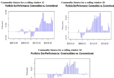
© 2015 AESS Publications. All Rights Reserved. 704 Commodity futures for a rolling window 12 Commodity futures for a rolling window 18
Commodity futures for a rolling window 24
Graph-3. Relative out-performance of portfolio with commodity futures Vs conventional asset class
Notes: This graph indicates the excess returns or losses of an optimal portfolio formed in the Mean-CVaR framework with and without commodities. The returns/losses are calculated from the opportunity investment cost given in equation (14). The percentage of relative loss is given in the x-axis and the time period is given in the y-axis. The positive percentage indicates that the Mean-CVaR optimal portfolio with commodities outperformed the Mean-CVaR optimal portfolio without commodities and vice-versa.
Opportunity excess returns of augmented portfolios were positive in most of the cases
suggesting that a premium needs to be paid by conventional asset portfolios to equalize the utility earned from portfolios made up of commodities.
The reduction in the weightage of energy and metal indices in the portfolio signals increased
financialization in these commodity sectors that reduced diversification benefits in the recent years. Contemporary research (Nissanke, 2012) deliberated that financialization was increased
substantially in commodity markets in the post crisis period since 2008 as commodities offered higher returns compared to other assets. These findings support the evidence of increased market
integration and reduced diversification benefits of alternative asset classes, viz. commodities during the crisis period.
Table 6.1 presents the diversification benefits of including individual commodity futures with the conventional assets for a rolling window of 12 months. Commodity futures, when added
individually, fail to generate higher Sharpe ratio than conventional assets. Diversification benefits lie in the combination of one or more commodity sectors. It was found that commodity portfolios exhibited time-varying nature in the relative outperformance (Graphs 3 and 4). During 2008 and
© 2015 AESS Publications. All Rights Reserved. 705 Table-6.1. Diversification benefits individual commodity futures
Portfolio performance
measures
Conventional Asset class
Agri Futures Metal Futures Energy
Futures Sharpe ratio
SR_SD 2.1769 2.0356 2.1175 2.0938
SR_CVaR 11.9605 5.6372 4.7236 5.2676
CDaR
Minimum 0.0015 0.0011 0.0012 0.0011
1st quad 0.0027 0.0016 0.0021 0.0015
Median 0.0038 0.003 0.0023 0.0016
Mean 0.0035 0.0042 0.0048 0.0044
3rd quad 0.0045 0.0043 0.0066 0.0066
Maximum 0.0053 0.0111 0.0118 0.0110
Opportunity returns/losses
Minimum -0.0165 -0.0177 -0.0208
1st quad -0.0094 -0.00 -0.0058
Median 0 0.0060 0
Mean -0.00207 0.0059 0.0041
3rd quad 0.0017 0.0146 -0.000003
Maximum 0.0186 0.0367 0.00164
Notes: This table reports the performance measures such as Sharpe ratio, conditional drawdown (CDaR) and opportunity returns/losses of Mean-CVaR optimized portfolio with conventional assets-Nifty 50 and Tbill and portfolio augmented with Comdex future indices and sub-indices namely, MCX Comdex, MCX Energy, MCX Metal and MCX Agri individually. Monthly observations are used in out of sample back-testing approach of Mean-CVaR optimization for rolling window 12.
Commodity metal futures for a rolling window 12 Commodity energy futures for a rolling window 12
Commodity agri futures for a rolling window 12
© 2015 AESS Publications. All Rights Reserved. 706 The weightages of Mean-CVaR optimization model for portfolios with commodity futures are given in Table 7. In Model 8 the conventional asset portfolio was augmented with all commodity
futures indices such as MCX futures, agri futures, metal futures and energy futures. Models 9 to 14 represent alternative combinations of various commodities. All the observations made in the spot analysis were further confirmed in the futures analysis regarding the continuous allocation of
agricultural sector in all the years. Energy futures received lower allocation compared to agri, and metals futures was allocated only during 2008-2011. However, the weightages of commodity
futures indices were relatively higher than commodity spot indices. The higher allocation to agri commodities can be substantiated from the correlation matrix given in Table 2, which indicates low
insignificant correlation with conventional assets. These results support the theory that bond markets are considered as the safe investments and highlight the emerging significance of agri
commodities in portfolio allocation. Though the weightages allotted to commodities were lesser in comparison to the conventional assets, it was found that commodity futures offered diversification benefits and help the investors to have better risk-return trade-off (Graph 3 and 4).
Table-7. Portfolio Compositions: Commodity futures and their combinations
Model-5. MCX Comdex futures
Assets/Year 2006 2007 2008 2009 2010 2011 2012 2013
Bond 0.79 0.707 0.747 0.675 0.714 0.67 0.694 0.761 Equity 0.21 0.29 0.24 0.29 0.25 0.30 0.28 0.22
Infrastructure 0.001 0.013 0.003 0.001 0.004
COMDEX futures
0.002 0.007
Metal futures 0.004 0.018 0.028 0.008 0.002
Energy futures 0.002 0.004 0.001 0.001 0.006 0.004 0.012 Agri futures 0.001 0.003 0.001 0.013 0.016 0.001
Model-6. Agri Futures
Assets/Year 2006 2007 2008 2009 2010 2011 2012 2013
Bond 0.72 0.769 0.707 0.731 0.682 0.765 0.778 0.700
Equity 0.28 0.23 0.28 0.24 0.29 0.21 0.2 0.29
Infrastructure 0.001 0.014 0.001 0.003 0.001
COMDEX futures 0.009 0.014 0.027 0.010 0.002 0.008
Agri futures 0.001 0.002 0.001 0.011 0.015 0.001
Model-7. Metal Futures
Assets/Year 2006 2007 2008 2009 2010 2011 2012 2013
Bond 0.79 0.8 0.738 0.766 0.744 0.785 0.744 0.71
Equity 0.21 0.2 0.25 0.2 0.22 0.20 0.25 0.28
Infrastructure 0.001 0.013 0.003 0.001
COMDEX futures
0.006 0.004 0.009 0.004 0.001 0.009
© 2015 AESS Publications. All Rights Reserved. 707 Model-8. Energy Futures
Assets/Year 2006 2007 2008 2009 2010 2011 2012 2013
Bond 0.79 0.768 0.75 0.722 0.682 0.714 0.772 0.731
Equity 0.21 0.3 0.24 0.25 0.29 0.27 0.22 0.25
Infrastructure 0.001 0.014 0.001 0.003 0.001 0.004 COMDEX
futures
0.005 0.014 0.027 0.011 0.003
Energy futures
0.002 0.003 0.003 0.003 0.012
Notes: The weights of respective Mean-CVaR optimized portfolios of conventional assets with commodity futures in different iterations are presented in this table. The monthly weights are averaged to get yearly portfolio weights for better understanding.
Diversification benefits were observed in commodity futures portfolios. The results are in sync
with the findings of Belousova and Dorfleitner (2012) and You and Daigler (2013). The diversification benefits of commodities are not uniform to all sectors across all time periods. Agri
futures, though not a standalone asset class, offers diversification benefits when combined with energy and metal futures respectively. The investment horizon has an impact on the portfolio
diversification benefits offered by commodities.
5. CONCLUSIONS
This study investigated the diversification benefits of commodities in the backdrop of the
uncertainty caused by the financial crisis and increased Financialization and speculation in the commodity markets. Extending the existing studies which employed static mean-variance optimization models this study deployed the stochastic Mean-Conditional Value at Risk
optimization framework. This model accounts for the uncertainty in the returns caused by different market conditions, the changing correlation nature between the assets and conditional value at risk
dynamics. Out-of-sample performance of the realized optimal portfolio across the asset classes was evaluated. The results indicate that the diversification benefits of commodities are more
pronounced with commodity futures than in spot markets. Metal and agri sectors were found to be offering better diversification compared to energy sector. The empirical results also provide
evidence that diversification benefits reduced during the financial crisis as cross asset markets were more integrated.
6. ACKNOWLEDGEMENT
The authors would like to gratefully acknowledge University Grants Commission, India and
DAAD, Germany for the support and fund provided by them to assist this research. The authors would like to acknowledge Prof. Hans Ziegler and Prof. C. Rajendran for their inputs during
research discussion.
REFERENCES
Belousova, J. and G. Dorfleitner, 2012. On the diversification benefits of commodities from the perspective of
© 2015 AESS Publications. All Rights Reserved. 708
Birge, J.R. and F.V. Louveaux, 1997. Introduction to stochastic programming. Ney York, Berlin, Heidelberg:
Springer Series on Operations Research.
Chong, J. and J. Miffre, 2010. Conditional correlation and volatility in commodity futures and traditional asset
markets. The Journal of Alternative Investments 12(3): 061--075.
Daskalaki, C. and G. Skiadopoulos, 2011. Should investors include commodities in their portfolios after all?
New evidence. Journal of Banking & Finance, 35(10): 2606-2626.
Erb, C.B. and C.R. Harvey, 2006. The strategic and tactical value of commodity futures. Financial Analysts
Journal, 62(2): 69-97.
Jensen, G.R., R.R. Johnson and J.M. Mercer, 2002. Tactical asset allocation and commodity futures. The
Journal of Portfolio Management, 28(4): 100-111.
Krokhmal, P., J. Palmquist and S. Uryasev, 2002. Portfolio optimization with conditional value-at-risk
objective and constraints. Journal of Risk, 4(2): 43--68.
Markowitz, H., 1952. Portfolio selection. The Journal of Finance, 7(1): 77--91.
Nissanke, M., 2012. Commodity market linkages in the global financial crisis: Excess volatility and
development impacts. Journal of Development Studies, 48(6): 732-750.
Sharpe, W.F., 1964. Capital asset prices: A theory of market equilibrium under conditions of risk. The Journal
of Finance, 19(3): 425-442.
Silvennoinen, A. and S. Thorp, 2013. Financialization, crisis and commodity correlation dynamics. Journal of
International Financial Markets, Institutions and Money, 24(0): 42 - 65.
Simaan, Y., 1993. What is the opportunity cost of mean-variance investment strategies. Management Science,
39(5): 578-587.
You, L. and R.T. Daigler, 2013. A markowitz optimization of commodity futures portfolios. Journal of
Futures Markets, 33(4): 343-368.
BIBLIOGRAPHY
Cheung, C.S. and P. Miu, 2010. Diversification benefits of commodity futures. Journal of International
Financial Markets, Institutions and Money, 20(5): 451-474.
Gorton, G. and K.G. Rouwenhorst, 2004. Facts and fantasies about commodity futures (10595). Technical
Report, National Bureau of Economic Research.
Rockfeller, T. and S. Uryasev, 2002. Conditional value-at-risk for general loss distribution. Journal of Banking
& Finance, 26(7): 1443-1471.
Simaan, Y., 1993. Portfolio selection and asset pricing—three-parameter framework. Management Science,
39(5): 568-577.