P
roblems
in
a
Fi
nancial
M
athematical
M
odel
Yasushi Ota
∗Okayama University of Science
Yu Jiang
†Shanghai University of Finance and Economics
Gen
nakamura
‡Hokkaido
University
Masaaki Uesaka
§Hokkaido University
February28,2019
Abstract
This paper investigates an inverse problem of option pricing in the extendedBlack–Scholes model. We identify the model coefficients fromthemeasureddataandattempttofind arbitrageopportunitiesin financialmarketsusingaBayesianinferenceapproach. Theposterior probabilitydensity functionofthe parametersis computedfromthe measureddata.Thestatisticsoftheunknownparametersareestimated byMarkov Chain MonteCarlo (MCMC),which explores the poste-riorstatespace. TheefficientsamplingstrategyofMCMCenablesus tosolveinverse problemsby theBayesian inferencetechnique. Our numerical results indicate thatthe Bayesian inference approach can simultaneouslyestimatethe unknown driftand volatilitycoefficients fromthemeasureddata.
Keywords and Phrases: inverse problem; option pricing;
Bayesian inference approach
1
Introduction
Financial derivatives are contracts that derive their value from the underlying as-set, such as stocks, bonds, commodities, and exchange rates. The behavior of the
∗This research was supported by KAKENHI (Grant number:18K03439). Faculty of
Manage-ment, Okayama University of Science, 1-1 Ridaicyou, Okayama City, Okayama Japan 700-0005, E-mail:[email protected]
†Address: School of Mathematics Shanghai University of Finance and Economics 777
Guod-ing Rd., Shanghai,200433, P. R. China (E-mail:[email protected])
‡This research was supported by KAKENHI (Grant number:19K03554). Faculty of
Sci-ence, Hokkaido University, nishi10 kitaku-kita20jyou Sapporo City, Hokkaido Japan 001-0020, E-mail:[email protected]
§
Faculty of Science, Hokkaido University, nishi10 kitaku-kita20jyou Sapporo City, Hokkaido Japan 001-0020, (E-mail:[email protected])
*Email:[email protected]
1
risk asset’s price is modeled by a diffusion processStsatisfying
dSt=µ(t, St)Stdt+σ(t, St)StdWt,
whereWtdenotes Brownian motion, andµandσare often called the volatility and
the drift(trend), respectively, of the risk asset’s price. Whenµandσ are positive constants,Stis called the Black–Scholes model.
As is well known, under the assumption that no–arbitrage property of a finan-cial market, the option priceu(t, S)is given by the following initial value problem : ∂u ∂t + 1
2σ(t, S)
2S2∂2u
∂S2 +rS
∂u
∂S −ru= 0, (t, S)∈[0, T)×(0,∞),
u(t, S)|t=T = max(0, S−K), S ∈(0,∞),
(1.1) where the interest rateris a nonnegative constant, andK is the strike price andT is the maturity of the underlying asset. The approach of the Black–Scholes model provides a useful, simple method of pricing inclusive of financial derivatives, risk premium, and default probability estimation. However, the theoretical prices of options with different strike prices which are calculated by the Black–Scholes equation differ from real market prices. In [6] and [18], taking this into account, we have extended Black–Scholes equation as follows :
∂u ∂t + 1
2σ(t, S)
2S2∂2u
∂S2 +µ(t, S)S
∂u
∂S −ru = 0, (t, S)∈[0, T)×(0,∞),
u(t, S)|t=T = max(0, S−K), S ∈(0,∞).
(1.2) In different real markets handling the same risk and asset, an arbitrage oppor-tunity often appears in the error µ−r. Practitioners may also request a conve-nience yieldµ−r from commodity markets. Suppose thatN arbitrage markets handle the same asset with pricesi(i = 1,2,· · · , N)at a given timet∗, we try to
identifyµ(Si)−rfrom the measured call option prices u∗(Si), at the same time t∗.
In this paper, our inverse problem seek the value ofµ(S)−rfrom given u(S, t)|t=t∗ =u∗(S), S ∈ω,
whereωis the interval andu(t, S)satisfies (1.2).
Inverse option problems (IOP) in mathematical finance were pioneered by Dupire [5]. Assuming no arbitrage, he derived the option premiumU(T, K)as a solutionu(·,·;T, K)to the dual equation of (1.2) with respect to the strike price K and maturity T as follows :
∂U
∂T −
1
2σ(T, K)
2K2∂2U
∂K2 +rK
∂U
If the option price and its derivative can be determined for all possibleT andK, then the local volatility functionσ(T, K)can be directly derived from Eq.(1.3) as
σ(T, K)2 =
∂U
∂T +rK
∂U ∂K
1 2K
2∂2U
∂K2
. (1.4)
Using this approach, we can deduce the local volatility function from the quoted option prices in the financial market. However, this strategy is impractical because we cannot get numerically stable data. In fact, since the data in financial markets are usually scarce and noisy, we cannot guarantee that the right–hand side of (1.4) remains constantly positive. Moreover the second derivatives of the option prices for all possible T and K are difficult to obtain, and their inverse problems are generally ill-posed. Using a linearization method, Bouchouev and Isakov [2], Bouchouev et al. [3], and Ota and Kaji [19] considered the following form of the time–independent local volatility functionσ2(K):
1 2σ
2(K) = 1
2σ
2
0+f(K)
wheref is a small perturbation of the constant σ0. They transformed (IOP) to a
Fredholm–type integral equation forf(K)and numerically determined the time– independent local volatility function. On the other hand, Mitsuhiro and Ota [18], Korolev et al. [12] and Doi and Ota [6] used the extended Black–Scholes equation (1.2) and then reconstructed the trend function by linearization method. The above studies provided point estimates of unknown parameters by exact determination or least squares optimization, without rigorously examining and considering the measurement errors in the inverse solutions. However, since most of the data in real financial markets are contaminated by measurement errors, uncertainties are ubiquitous. Further errors are introduced by linearizing the inverse problems or the inverse methodology; for example, discretizing the integral equation obtained by the linearization method.
Dupire’s method [5] requires the solution at all points or the second order gradient of the solution. On the other hand, MCMC method can avoid having this. Rather than applying a Dupire–type formula or the linearization method, we attempt a parameter reconstruction by a statistical method that simultaneously estimates the unknown trend and volatility coefficients from the measured data. In other words, we seek arbitrage opportunities by simultaneously estimating the gap in the given interest rate and the volatility. If our results reveal the existence of an arbitrage, then a profitable trading strategy in real financial markets is expected.
This paper is divided into five parts. Our inverse problem is mathematically formulated in Section 2. Section 3 outlines the general Bayesian framework for solving inverse problems and discusses the numerical exploration of the posterior state space by the MCMC method. In Section 4, we discretize our inverse problem and reconstruct the parameters by a numerical algorithm. We then discuss various aspects of our results through numerical examples. Concluding remarks are given in Section 5.
2
Inverse option problems
This section formulates an inverse problem which is defined in Introduction. In the following problem, the local volatilityσ(t, S) is a positive constant σ0 > 0
and the trend µ(t, S) is a time–independent function in (1.2) under the suitable condition:
u(t, S)|t=T = max{S−K,0}, (2.1)
whereK is the stock price at the maturity dateT. Upon the following change of variables and substitutions,
y= log S
K, τ =T −t, (2.2)
then, the equation and initial condition of (1.2) in terms of
µ(y) = µ(Dey), U(τ, y) = u(T −τ, Key)/D (2.3) becomes
∂U
∂τ =
1 2σ
2 0
∂2U
∂y2 − (1
2σ
2
0 −µ(y) )∂U
∂y −rU, (τ, y)∈(0, τ
∗)×R,
U(τ, y)|τ=0 = max{ey −1,0}, y∈R,
(2.4)
U(τ∗, y) =U∗(y), y∈ω ⊆R,
our IOP, Eqs. (2.4) and (2.5) seek the values ofµ(y) =r+f(y)andσ0from the
givenU∗(y), wheref is a small perturbation of the interest rater.
However, due to the nonlinearity of this inverse problem, the uniqueness and existence of its solution are hard to prove. The present paper attempts to recon-struct the parameters by a statistical method simultaneously estimates µ(y) =
r+f(y)andσ0from the measured dataU∗(y). In other words, we seek arbitrage
opportunities by simultaneously estimating the gap from the given interest rate and the volatility.
Let us definem−dimensional vectorsY,F(θ)andεas follows :
{Y}j = U∗(yj) = U(τ∗, yj; ¯θ)(1 +εj)
{F(θ)}j = U(τ∗, yj;θ)
{ε}j = εj
where yj(j = 1,· · · , m) are the measurement points at τ∗, U(τ∗, yj;θ) solves
the Cauchy problem (2.4) for the unknown parametersθandεj is the uncertainty
(noise) in the market, assumed as white Gaussian noise. We then seek the param-etersθ¯, which assumedly represent the true value ofθ, such that
Y ≃F(θ) +ε. (2.5)
3
Bayesian inference approach to the IOP
Recently, the Bayesian inference approach has been greatly extended through the development of analytical techniques such as MCMC (see [11]).
The Bayesian inference approach considers the parameters not as single val-ued, but as a probability distribution. The above–mentioned PPDF defines the parameter probability distribution estimated from the measured data. Mathe-matically, the PPDF is expressed as f(θ|Y) and is the product of the likelihood functionf(Y|θ) and the prior density functionf(θ). The underlying concept of Bayesian inference is Bayes’ theorem, which relates the parametersθand the ob-served dataY as follows:
f(θ|Y) = f(Y|θ)f(θ)
f(Y) . (3.1)
Equation (3.1) states that given some observationsY, the posterior probability of a hypothesis is proportional to the product of its likelihood and its prior probability. The present paper assumes that the random errors in Eqs. (2.5) are white Gaus-sian noise with a known standard deviationΣε. The likelihood functionf(Y|θ)is
then given as
f(Y|θ) = exp
{
−(Y −F(θ))T(Y −F(θ))
2Σ2
ε
}
The prior density function is simply assumed as f(θ) = U[−θ0,θ], whereθ0 is a sufficiently large positive constant. The PPDF of the parametersθ can be written as follows:
f(θ|Y)∝exp
{
−(Y −F(θ))T(Y −F(θ))
2Σ2
ε
}
. (3.3)
Here, the standard derivationΣεis known and can be regarded as a regularization
parameter.
3.1
MCMC methods
In Bayesian inference, the complicated and intractable probabilistic models can be estimated by numerical sampling methods such as MCMC, which has been widely applied in recent years. The details of MCMC methods are given in Robert and Casella [20].
Monte Carlo simulation generates pseudo–random numbers for exploring pos-terior distributions. In the MCMC algorithm, the pseudo–random number is a Markov chain. The MCMC algorithm exploits the property of a Markov chain to generate pseudo–random numbers from a posterior distribution, even for a com-plicated model. It first constructs an ergodic Markov chain with a stationary distri-bution equaling the target distridistri-bution. By iterating the Markov chain transitions from suitable initial value, it eventually obtains the target distribution.
This paper employs a typical MCMC algorithm called the Metropolis–Hastings (M–H) algorithm (see Metropolis et al. [17]; Hastings [9]). The M–H (Algorithm 1) given below builds its Markov chain by accepting or rejecting samples ex-tracted from a proposed distribution. This algorithm is generally used in Bayesian inference and is a powerful tool for solving inverse problems (cf. [11]).
Algorithm 1Metropolis-Hastings MCMC
1: Generate θ′ ∼ q(·|θk) = N(θk, σ2θ) (the normal distribution) with a given
stander derivationσ >0for givenθk.
2: Calculate the choiceα(θ′, θk) = min{1, f(θ′|Y)/f(θk|Y)}.
3: Updateθkasθk+1 =θ′with probabilityα(θ′, θk)but otherwise setθk+1 =θk.
By running the M–H algorithm, we can sample the distribution f(θ|Y), and usually the mean value of θk, after a given burn-in time k∗. Unlike common
4
Numerical examples
In this section, we generate numerically an exact artificial data setF(θ)and let (4.2) be the numerical data, where random errorεcontains both the random mea-surement error and the numerical error.
In the rest of this paper, we assume the trendµ(y)has the form :
µ(y) =r+µ1y, (4.1)
whereµ1 is the unknown constant. We also assume the measurement dataY has
the form :
Y =F(θ) +ε, (4.2)
where random error ε contains both the random measurement error and the nu-merical error. By reconstructing the parameters by the M–H method, we simulta-neously estimateµ1 andσ0 from the measured dataY in Eqs.(4.2).
4.1
Direct problems
In this section, we assume r = 0 and solve the direct problem for (2.4) by the numerical Crank–Nicholson scheme :
ajUi+1,j+1+ (1 +b)Ui+1,j+cjUi+1,j−1
=−ajUi,j+1+ (1−b)Ui,j−cjUi,j−1, (4.3)
whereUi,j =U(ti, yj),and
aj =− ∆τ
4 (∆y)2
{
σ0+ ∆y (
−1
2σ0+µ1yj
)}
,
b = ∆τ
2 (∆y)2,
cj =− ∆τ
4 (∆y)2
{
σ0−∆y (
−1
2σ0+µ1yj
)}
.
Here, we took a uniform grid
˜
ω ={(τi, yj) :τi ∈(0, τ∗), yj ∈I15= (−15,15),
i= 1,2,· · · , M, j = 1,2,· · · ,200}
with artificial zero Dirichlet boundary conditions at y = −15and15, and∆τ =
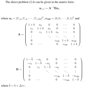
The direct problem (2.4) can be given in the matrix form :
ui+1 =A−1Bui, (4.4)
whereui= (Ui,2, Ui,3,· · · , Ui,199)T,e198= (0,0,· · · ,0,1)T and
A=
1 +b a2 0 0 · · · 0
c3 1 +b a3 0 · · · 0
0 c4 1 +b a4 · · · 0
..
. . .. . .. . .. ...
0 c198 1 +b a198
0 · · · 0 c199 1 +b
, B=
1−˜b −a2 0 0 · · · 0
−c3 1−˜b −a3 0 · · · 0
0 c4 1−˜b −a4 · · · 0
..
. . .. . .. . .. ...
0 −c198 1−˜b −a198
0 · · · 0 −c199 1−˜b
,
where˜b =b+ ∆τ r.
4.2
Inverse problem solution by MCMC
Table 1 shows the true values and parameter settings in Algorithm 1.
Table 1: Parameter setting in Algorithm 1.
True value µ1 1 σ0 1
Others Σε 10−3 σθ (0.01,0.01)
In the following examples, the relative noise in all the observations Y is as-sumed as5%and the prior distributionf(θ)of unknowns is(µ1, σ0) = 1. That is,
we can sayfprior(θ) =1[µmin
1 ,µmax1 ](µ1)·1[σmin0 ,σ0max](σ0)and the intervals[µ
min 1 , µmax1 ]
and [σmin
0 , σ0max] are large enough so that all (µ1, σ0)’s appearing in the Markov
chain fall into these intervals. Here, we set the the indicator function as
1A(a) =
{
1 a∈A,
General uniform distributions can be used forf(θ)if we use the prior-reversible proposal that satisfiesf(θ)q(θ′|θ) = f(θ′)q(θ|θ′)(see for example [10]). On the other hand, if we choose f(θ)as a Gaussian distribution, this will turn out to be the Tikhonov regularization term in the cost function.
For comparison, we particularly consider the Levenberg-Marquardt algorithm [13, 15]. That is, the recovery ofθ= (µ1, σ0)T is computed by the iteration given
by
θk+1 =θk+
[
F′(θk)TF′(θk) +λI
]−1
F′(θk)T(U −F(θk)), (4.5)
whereF′(a)is the Jacobian matrix and the parameterλ is nonnegative. This al-gorithm can be implemented by an inner embedded programlsqcurvefitin MAT-LAB®2018a.
Example 1:
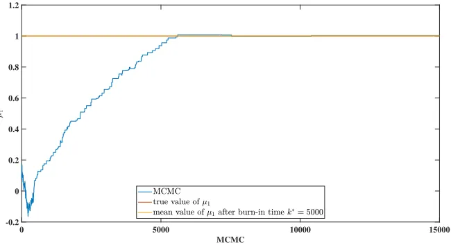
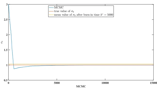
The MCMC sampled(µ1, σ0)is shown in Figures 1 and 2, respectively. The
recovered result is given in Table 2 showing a good recovery. For comparison, the converged recovery of(µ1, σ0,)obtained by the Levenberg–Marquardt algorithm
is also provided in Table 2.
0 5000 10000 15000 MCMC
-0.2 0 0.2 0.4 0.6 0.8 1 1.2
0 5000 10000 15000 MCMC
0 0.2 0.4 0.6 0.8 1 1.2
Figure 2: MCMC sampling of the parametersσ0
Table 2: Recovery results of(µ1, σ0).
µ1 σ0
Initial guess 0.1 0.1
Mean value after burn-in timek∗ = 5000 1.0008 1.0002 Result of Levenberg–Marquardt algorithm 1.0020 1.0001
True value 1 1
Example 2:
In this example, the initial guess of (µ1, σ0) was set to a value far from the
true value(1,1). The evolutions of the MCMC sampledµ1 andσ0 are shown in
Figure 3 and 4, respectively, and the recovered result is shown in Table 3. Again, the recovery of(µ1, σ0)is good. The divergent recovery of(µ1, σ0)obtained by
0 5000 10000 15000 MCMC
0.5 1 1.5 2 2.5 3 3.5
Figure 3: MCMC sampling of the parameterµ1.
0 5000 10000 15000
MCMC 0.5
1 1.5 2 2.5 3
Figure 4: MCMC sampling of the parameterσ0
Table 3: Recovery results of(µ1, σ0).
µ1 σ0
Initial guess 3 3
Mean value after burn-in timek∗ = 5000 1.0341 0.9976 Result of Levenberg–Marquardt algorithm 4.2334 1.0579
From the MCMC samples in Figures 1 – 4 and the recoveries obtained by the Levenberg–Marquardt algorithm (especially in Table 3), we observe thatµ1 is
more sensitive to noise thanσ0 and hence it is less easily recovered.
5
Conclusion
This paper verified the effectively of the Bayesian inference approach to IOP. The posterior distributions of the unknown trend and volatility coefficients were re-covered from the measured data by modeling the measurement errors as Gaussian random variables. The posterior state space was explored by the M–H method. As confirmed in the numerical results, the Bayesian inference approach simulta-neously estimated the unknown trend and volatility coefficients from the measured data.
The method presented here can be extended in several ways. Our immediate future work will statistically apply the Tikhonov regularization method to IOP. As the hierarchical Bayesian method is analogous to the Tikhonov regularization method, it enables the automatic selection of the regularization parameter. Next, we will develop mathematical theories (for instance, the uniqueness, stability, and existence) of IOP and extend our approach to two–dimensional cases. Finally, the model should be tested in a trading strategy using real market data.
Acknowledgments
The first author would like to acknowledge the supports from JSPS Grant-in-Aid for Scientific Research (C) 18K03439. The second author was supported by National Natural Science Foundation of China (No. 11771270). The third author would like to acknowledge the supports from Grant-in-Aid for Scientific Research (15K21766 and 15H05740) of the Japan Society for the Promotion of Science (JSPS).
References
[1] Black F and Scholes M. 1973The pricing of options and corporate liabilities Journal of Political Economy.81, 637-659
[3] Bouchouev I, Isakov V and Valdivia N. 2002Recovery of volatility coefficient by linearization Quantitative Finance.Vol2 257-263
[4] Cui T, Fox C, and O?fSullivan MJ. 2011Bayesian calibration of a large-scale geothermal reservoir model by a new adaptive delayed acceptance Metropolis
Hastings algorithm Water Resource Research47W10521
[5] Dupire B. 1994Pricing with a smile Risk.7 18-20
[6] Doi S and Ota Y. 2018Application of microlocal analysis to an inverse prob-lem arising from financial markets Inverse Probprob-lems.34N11
[7] Friedman A. 1983 Partial Differential Equations of Parabolic Type. (Engle-wood Cliffs, N.J : Prentice-Hall)
[8] Haario H, Laine M, Lehtinen M, Saksman E and Tamminen J. 2004Markov chain Monte Carlo methods for high dimensional inversion in remote sensing Journal of the Royal Statistical Society: Series B (Statistical Methodology).
66591-608
[9] Hastings, W. 1970Monte Carlo sampling methods using Markov chains and their application Biometrika.5797-109
[10] Iglesias M A, Lin K and Stuart A M. 2014Well-posed Bayesian geometric inverse problems arising in subsurface flow Inverse Problems30, 114001
[11] Kaipio J and Somersalo E. 2005Statistical and Computational Inverse Prob-lems.(New York : Springer)
[12] Korolev M, Kubo H and Yagola G 2012Parameter identification problem for a parabolic equation-application to the Black-Scholes option pricing model J. Inverse Ill-posed probl.20No.3 327-337
[13] Levenberg, K. 1944A method for the solution of certain non-linear problems in least squares Quarterly Appl. Math.2, 164–168
[14] Lishang J and Youshan T. 2001Identifying the volatility of underlying assets from option prices Inverse Problems.17137-155
[15] Marquardt D. 1963.An algorithm for least-squares estimation of nonlinear parameters SIAM J. Appl. Math.11, 431–441.
[17] Metropolis N, Rosenbluth A, Rosenbluth M, Teller A and Teller E. 1953 Equations of state calculations by fast computing machines J. Chem. Phys.
21(6)1087-1092.
[18] Mitsuhiro M and Ota Y. 2015 Recovery of Foreign Interest Rates from
Ex-change Binary Options Computer Technology and Application676-88
[19] Ota Y and Kaji S. 2016Reconstruction of local volatility for the binary op-tion model J. Inverse Ill-posed probl.24No.6 727-742
[20] Robert.C and Casella.G 2004 Monte Carlo Statistical Methods (Springer Texts in Statistics)
[21] Wang J and Zabaras N. 2004A Bayesian inference approach to the inverse heat conduction problem International Journal of Heat and Mass Transfer.
47, Issues 17-18, 3927-3941