Junction Detection: Computation and Psychophysics
by
Joshua Hartman McDermott
Submitted for the Degree of Mphil
at
University Colledge London
ProQuest Number: U643289
All rights reserved
INFORMATION TO ALL USERS
The quality of this reproduction is dependent upon the quality of the copy submitted. In the unlikely event that the author did not send a complete manuscript and there are missing pages, these will be noted. Also, if material had to be removed,
a note will indicate the deletion.
uest.
ProQuest U643289
Published by ProQuest LLC(2015). Copyright of the Dissertation is held by the Author. All rights reserved.
Abstract
Junctions, formed at the intersection of image contours, have been thought to play an important
and early role in vision since the time of Helmholtz, and have recently been the focus of much
research in vision science. The interest injunctions can be attributed in part to the notion that
they are local image features that are easy to detect which nonetheless provide valuable
information about important scene events like occlusion and transparency. Despite the
prevalence of this view, the extent to which it holds for junctions in real images remains unclear.
In this thesis we put this notion to the test. Our first approach involves psychophysical
experiments with real images as stimuli in which we use the human visual system as a tool to
measure the visual information available in local image regions. W e test the ability of observers
to detect occlusion points, which by hypothesis are signified by local junctions, given only a
small image region surrounding the occlusion point. Human performance in our experiments
places constraints on how junctions might be detected and what their role in vision might be. We
also attempted to train neural networks to detect junctions given only a small image patch
centered on the junction. Together, our experiments suggest that although some junctions are
locally defined and can be detected with simple and local mechanisms, a substantial fraction
necessitate the use of more complex and global processes, and may not play the bottom-up role in
Table of Contents
Abstract
2
1 Introduction
4
2 Psychophysics with Real Images
7
2.1 Stimulus Acquisition 7
2.2 Experiment 1: Aperture Size 9
2.3 Illustrative Example Stimuli 17
2.4 Experiment 2: Controls 21
3 Psychophysics Experiments on Scale
24
3.1 Experiment 3: Scale 24
3.2 Scale Examples 29
3.3 Scale Artifacts 36
3.4 Nonlocal Occlusion Points 41
3.5 Scale Selection 45
3.6 General Discussion of Psychophysics 47
4 Neural Networks for Junction Detection
51
4.1 General Motivation 51
4.2 Network Implementation 54
4.3 Training on Real Points of Occlusion 56
4.4 Training on Synthetic Junctions 61
5 Rotation Invariant Neural Networks
66
5.1 Training on a Single Orientation 66
5.2 General Discussion of Neural Networks 71
6 Conclusions
73
Acknowledgements
75
Chapter 1: Introduction
Vision is the task o f inferring representations of scenes in the world from images. Doing this
properly involves implicitly estimating a probability distribution o f scenes given an observed
image, and perhaps searching through the space of scenes to find the one that is most likely or in
some other sense best given the distribution. The problem, o f course, is that the direct estimation
o f this distribution is intractable due to its high dimensionality - a huge num ber o f parameters is
required to describe an entire scene. Moreover, searching through the space of scenes is also
intractable, again due to the high dimensionality. A more promising alternative is to estimate
many reduced versions of this distribution at different locations in an image, i.e. to estimate at
each location the distribution over the local scene parameters (e.g. surface curvature, reflectance,
etc.) given the image region at that location. Such local distributions are (hopefully) more
tractable to estimate and use because of the smaller number o f parameters involved. Locally the
distribution of scene structure given the image is less peaked and unimodal because there is less
information to constrain scene interpretation. However, the local distributions could narrow the
possible interpretations and might then be combined to yield a global scene estimate. Methods
have recently been suggested that accomplish this in some simple cases (e.g. Saund, 1999;
Freeman, 2000).
Something akin to this broad strategy seems likely to play a large role in vision; the big search
involving the entire image is too hard, and yet we manage to see astoundingly well, implying that
shortcuts are available and are taken by biological visual systems. The hierarchical nature of
mammalian visual systems may also be reflective o f such a strategy. The main question, then, is
just whether the local processing will be intelligible, i.e. whether vision science will be able to
produce a blueprint for what happens locally. It might be the case that the local processes are
messy and difficult to make sense of, but the assumption implicit in much o f vision research is
that this is not the case. It is for this reason that there is much interest in local cues such as
junctions.
Junctions, formed at the intersections of image contours, are attractive candidates for elements of
early vision because they are presumed to be local image features which nonetheless provide
substantial information about many important scene characteristics. Junctions have been
Anandan, 1990; T-junctions, Anderson, 1997), and reflectance, illumination, and atmospheric
boundaries (T-junctions, Gilchrist, 1979; X-junctions, Adelson, 1993, 1999). Furthermore,
junctions lend themselves to appealingly principled and rule-driven models o f many aspects of
mid-level vision (e.g. Sajda and Finkel, 1995).
Although a growing body o f psychophysics suggests an important role for local junction analysis
in mid-level vision, virtually all the psychophysical and modeling work on junctions is conducted
with "cartoon" images composed of discrete luminance values and step edges. W hile these may
be a useful abstraction of real images, it is unclear how representative the junctions in such
images are of junctions in real images. For junctions to be used in the manner that the simple
models and psychophysics suggest, they must be locally discernible, and yet it is not obvious that
this is the case in real images. Psychophysicists are happy to point out junctions in real images,
but in doing so are making use of the entire image and their entire visual system. It might be the
case that a substantial fraction of junctions become visible only after the image in which they lie
is interpreted, in which case the theoretical claims that have been made about them would be
called into question.
One obvious approach to investigating this issue is to attempt to design a mechanism for
detecting junctions in real images, in that the success of a local m echanism at detecting junctions
would imply that they are indeed locally defined. However, the results o f several previous such
attempts have been discouraging (Beymer, 1989; Heitger et al., 1991; Freeman, 1992; Alvarez
and Morales, 1997; Lindeberg, 1998; Farida et al., 1998). Sensible computations involving
oriented filtering and local templates result in apparently poor performance on real images. This
is surprising given that much o f the interest in junctions is predicated on their apparent simplicity.
These results might be taken to indicate that there is insufficient information in local regions of
real images to detect junctions. Note, though, that there is an inherent difficulty in claiming on
the basis of failures in machine vision that a low-level/local mechanism is insufficient to do some
1986; Zucker et al., 1988; Shashua and Ullman, 1990). Recently there have been further attempts
to refine the local operators (Iverson and Zucker, 1995). Although it is generally agreed that
some degree of nonlocal post-processing is necessary to generate edge maps suitable for further
analysis (e.g. inferring shape from contours), it is not clear how well a local operator should be
expected to perform, in part because they are typically evaluated by looking at their outputs in the
context of an entire image. It is thus difficult to ascertain the extent to which more sophisticated,
nonlocal analysis is needed.
Traditional psychophysics experiments on people, in contrast, can help by demonstrating the
existence of novel mechanisms in human vision, using cleverly designed stimuli that low-level
mechanisms are provably unable to deal with. Classic examples o f this include second-order
stimuli, which can demonstrate the existence o f texture-based mechanisms for edge detection, and
the association field stimuli of Field, Hayes and Hess (1993), which have been used to
demonstrate "contour integration" in human vision. Such findings can be useful for machine
vision because the existence of such mechanisms in human vision suggests that vision problems
may necessitate them. However, this approach has its own shortcomings, the main one being that
there is no way o f knowing the extent to which such mechanisms are active outside the lab in the
presence of real world stimuli. There are many people who contend, for instance, that second-
order mechanisms for motion are largely epiphenomenal in normal vision.
In this thesis we take an alternative approach: psychophysics with real images as stimuli. We
contend that psychophysics with real images can complement machine vision and traditional
human psychophysics by showing what human observers can and can’t do given some fraction of
the information available in real images. Simple manipulations (filtering, masking etc.) can be
used to restrict the information available to an observer. An observer’s competence at a task is an
existence proof that it can be done given the restrictions, whereas failure suggests that it cannot.
W e first present a series of experiments within this paradigm which provide insights and
constraints on junctions and their detection. W e then attempt to leam junction detectors given the
Chapter 2: Psychophysics
The goal o f our psychophysics experiments was to examine the extent to which occlusion in real
images produces simple and local cues like junctions that might be easily detected by early visual
mechanisms. Junctions are purported to be locally discernible image features, and we wanted to
put this notion to the test. The main idea is straightforward: if junctions are locally defined, then
observers should be able to reliably detect them given only a small image region centered on the
junction.
To test this idea, we first needed a large set o f junction candidates to use as stimuli. Junctions
are, by hypothesis, generated by significant events in the world such as the occlusion of one edge
by another, so this is where we looked for them. W e restricted our study to junctions generated at
points of occlusion, because this is by far the most common junction-generating situation
occurring in real scenes; such points were plentiful enough to study in some detail. It was also
fairly easy to describe to observers how they should label a point o f occlusion. W e thus began by
having naive observers identify points of occlusion in natural images.
2.1 Stimulus Acquisition
Observers were asked to label the points in an image where "one edge occludes another", a task
that tended to be intuitive and natural for naive observers to do. Their instructions were as
follows:
"In each image you should label the "points of occlusion". A point of occlusion is defined as a
point in an image where one edge is occluded by (i.e. goes behind) another. The occluding edge
will be the border of a surface or object, but the occluded edge (i.e. the one that goes behind) can
be any sort o f edge (e.g. a surface marking such as paint, the borders o f shadows, etc., in addition
thin as to make it impossible to distinctly label the two points of occlusion occurring on each side
of the line, subjects were instructed to take the center of the line to be the point of occlusion.
Such locations were obtained for 20 real images taken from the online database of Van Hateren
(Van Hateren and van der Schaaf, 1998) consisting of images of various locations in the
Netherlands taken with a digital camera. Images were logarithmically transformed and scaled for
display purposes. We selected images which appeared to have lots of occlusion points. Some
contained buildings and other man-made objects, whereas others consisted mainly of trees and
plants. Most images were labeled by two observers, and labels tended to be consistent across
observers. We then sifted through the sets of locations to eliminate the occasional erroneous label
as well as to ensure that the locations were centered as well as was humanly possible. In the end
we accumulated approximately 1200 occlusion points. An example image with labels is shown in
Figure 2.1.
A''
-mm
These labeled points were all locations where occlusion could be seen upon inspection of the
entire image at once. To test for the presence of local signatures of occlusion, such as T-
junctions, we asked observers to detect occlusion points given only a small image region
surrounding them.
2.2 Experiment 1: Aperture Size
Observers were presented with a succession of image patches of varying size. For each patch,
they were asked to guess whether it was centered on an occlusion point. Some of the patches
were centered on the previously labeled occlusion point locations, some were selected randomly
from the same images, some were synthetic edges, and some were synthetic T- and L-junctions.
If points of occlusion are signaled by a local image signature such as a T-junction, subjects
should perform well on an occlusion discrimination task even for small apertures. Furthermore,
the synthetic stimuli can help us characterize what subjects are basing their judgment on. If
subjects are using T-junctions to detect point of occlusion, then they should also classify the
synthetic T-junctions, but not the L-junctions, as occlusion points.
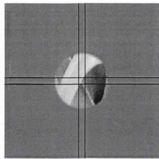
Figure 2.2. Example experimental display. Patch is 97 pixels wide.
Methods
hairs could be moved in front of the image when localization was in doubt, as shown in Figure
2.3.
Figure 2.3. Example experimental display with crosshairs toggled in front.
Subjects were given the following instructions:
"The purpose of this experiment is to leam how the human visual system detects occlusion
relationships in the world. We are particularly interested in whether the locations where one
object occludes another can be detected using very local information in an image. In the first
stage of this study, several observers labeled "occlusion points" in a series of images of the world.
In the present experiment, you will be presented with a series of image patches of varying size,
taken from the images that were labeled in the first stage of the study. Some of these patches will
be centered on the previously labeled occlusion points, while some will be centered on randomly
selected locations. Of the latter, some will contain just a single edge, some will be regions of
texture, some will be blank, and some will contain occlusion points that are not centered on the
patch. You will be asked to guess whether a given patch is centered on an occlusion point. In
some cases this will be obvious, and others less so."
The randomly selected patches were drawn randomly from the same images from which the
occlusion points were obtained, subject to the constraint that the standard deviation of the
intensities of the central 13 by 13 pixels exceeded 10 (intensities ranged from 0-255). This was to
reduce the number of "uninteresting" patches (e.g. those that were essentially uniform) that could
be trivially distinguished from occlusion points. The synthetic edges and junctions were
generated in Matlab. The different sectors o f the junctions and edges were uniform in luminance
the 0-255 scale, to ensure that the junctions and edges were well above threshold. The stimuli
were generated at large sizes and blurred and subsampled to reduce aliasing. A small amount of
noise was then added (normally distributed with a standard deviation o f 5). Because they were so
easy to see, the synthetic stimuli were only displayed at the three smallest aperture sizes. The
proportions of stimuli in the experiments were as follows: 40% o f the patches were centered on
real point of occlusion, 45% were randomly selected patches o f real images, and there were 5%
each of synthetic edges, L-junctions, and T-junctions.
Patches were displayed at one o f 5 sizes (13, 2 5,49, 97, or 201 pixels in diameter) on a uniform
background set to slightly above or below the mean luminance o f the patch. This was achieved
by multiplying each image region with a circular mask. At the borders the mask faded gradually
to zero over a 5 pixel radius increment. (Note that as a result, the effective size of each patch was
roughly 4 pixels greater than the listed size.) Stimuli were generated and displayed in Matlab on
a PC running Linux. Patches were displayed at full resolution on a Yama Vision M aster Pro 450
m onitor in ambient illumination. Subjects were instructed to sit at a comfortable viewing
distance. This was usually a bit less than arm ’s-length, at which the smallest patch size subtended
roughly 0.25 degrees visual angle. On each trial the display was present until subjects entered
their responses; viewing time was unlimited.
Subjects entered two responses on each trial. They were first asked to make their best guess as to
whether the current patch was centered on an occlusion point or not, by pressing one of two
buttons. They were then asked to make a confidence rating, pressing one of three buttons to
indicate whether they were essentially guessing, somewhat sure, or quite sure that their previous
judgm ent was correct. Subjects were instructed to envision a continuum o f confidence and to
assign thirds of that continuum to each button. Each response was confirmed with a second key
press before which subjects had the option o f changing the response. This was intended to
minimize mistaken responses, and seemed to be effective: subjects were debriefed following each
experiment and consistently claimed to have made only a handful of such mistaken responses.
classifications ju st on the basis of an edge running through the center of the patch. No feedback
was given on trials with synthetic junctions, since these were intended as a barometer of a
subject’s strategy. Subjects were told that the feedback signal was probabilistic (i.e. would not
occur for every error), to be consistent with the absence o f feedback on these trials. Subjects
were told the following about the feedback:
"To help you perform the task as well as you can, on some trials you will be given feedback. The
computer will sometimes make a buzzing sound when you incorrectly label the current patch.
You should try to take this feedback into account as you decide how to respond. There may be
particular patterns that occur at points of occlusion that you can use to detect them."
Subjects began their participation in the experiment by completing roughly an hour’s worth of
practice trials. Once fully comfortable with the judgm ents and response requirements, each
subject completed approximately 700 experimental trials. The subjects who participated in the
experiments were different from the subjects who labeled the images, and had never seen the
images from which the patches were extracted. W e collected data from 5 subjects.
Results
The data from all 5 subjects were qualitatively similar, and were combined for analysis purposes.
Figure 2.4a plots classification errors for the real image patches as a function of the aperture size.
At the smallest aperture size (13 pixels in diameter), subjects misclassify 27 percent of the image
patches (chance performance is 50 percent). Errors drop gradually as the aperture size is
increased, but do not reach a minimum until an aperture size of about 100 pixels. Figure 2.4b
plots histograms o f subjects’occlusion judgm ents for the real image patches, divided into patches
that actually were points o f occlusion and those which were randomly selected. Most of the
effect of aperture size is on misses: points o f occlusion that are not classified as such. At the
smallest aperture size, just over half of the patches that are in fact centered on points of occlusion
are correctly classified; this proportion increases to over 90 percent at the largest aperture size.
Note that all of these image patches were clearly points of occlusion when the entire image was
viewed at once; this was the criterion by w hich they were labeled. The fact that subjects
misclassify a small proportion of the occlusion points at the largest aperture size tested implies
that a degree of ambiguity exists even for this large size (otherwise subject would have been close
a
40
6 20
Figure 2.4. Results of Experiment 1.
Occlusion Classification of Real Image Patches
T otal Errors Results for 5 subjects
1 I r
I
12.1
13 25 49 97
<—Patch Diameter in Pixels—>
11
201
b
100
I
o 50 H
I
13 25Ju d gem en ts fo r Points o f O cclu sion
J
1
49J
1
97 J1 201Ju d g em en ts fo r R an d om Points 100 0 Q.
1
O H oI
9713 25 49 201
<—Patch Diameter in Pixels—>
■ Judged as Ctelusion Points □ NOT Judged as Occlusion Poirts
occlusion are randomly selected. Occasionally, locations are randomly selected that happen to lie
on points of occlusion. W ith purely random selection this would be a very improbable event, but
as described above, the patches were also constrained to have high variance in their pixel
intensities, which predisposed the selection process towards edges and other regions of high
contrast. Moreover, subjects were given intentionally lax guidelines with regard to the centering
of the occlusion points: they were instructed to classify something as being centered on an
occlusion point if there appeared to be such a point within the cross hair boundaries, a 10 by 10
pixel region. This made it easier still for randomly selected patches to legitimately contain
occlusion points. Thus many o f the "random" points that were classified as occlusion points were
classified correctly, and are not true false positive responses. The only way to get around this
would be to painstakingly weed out these points by hand, which we did not do. W e are thus
clearly overestimating false positive rates; this is a weakness of the method.
Our qualitative results are quite clear, however: even when forced to guess, human observers are
unable to identify many points of occlusion just on the basis of local information. This suggests
that in many cases there isn’t much o f a local cue such as a T-junction with which to detect the
occlusion. Conversely, though, in many cases observers can reliably identify occlusion points
with purely local information, providing an existence proof for local cues of some sort. It would
be of interest to characterize the nature o f such cues. However, our occlusion discrimination task
could conceivably be performed with any number of different strategies, and our results with real
image patches provide few constraints on the strategies our subjects could be adopting. Synthetic
Figure 2.5. Results of Experiment 1 for synthetic stimuli.
§
100 <u CE: o HI
500
Occlusion Judgements for Synthetic Junctions
T -Junctions
_CL
13 25 49
<—Patch Diameter in Pixels—>
L -Junctions
100
50
0
<—Patch Diameter in Pixels—>
■ Judged as Ct elusion Points □ NOT Judged as Occlusion Poirts
Figure 2.5 shows occlusion judgments for the synthetic junctions inserted as "catch trials" in the
experiments. In contrast to the real image patches, the classification of the synthetic junctions
depends very little on aperture size. Virtually all of the T-junctions are classified as occlusion
points whereas most of the L-junctions are not. Note that this does not show that observers’
judgments on the real points of occlusion are mediated by junctions; they could very well be
monitoring other things. It is, however, consistent with the notion that junctions are involved.
Moreover, it suggests that if junctions were present at most points of occlusion in real images,
observers would make use of them within our paradigm to identify the occlusion points as such.
Thus the fact that they fail to pick out many of the occlusion points suggests that junctions are not
visible there.
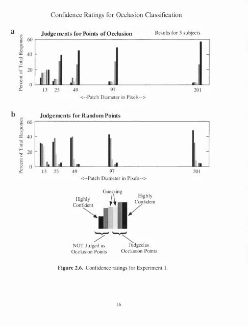
Figure 2.6 plots histograms of our observers’ confidence ratings in each experimental condition.
For display purposes, the ratings were combined with the occlusion judgments, such that the six
aperture size, the majority of judgments are very confident and correct. There is a similar but
weaker trend evident in the responses for the randomly selected patches. In contrast, the vast
majority of the confidence ratings for the synthetic junctions are high, for both small and large
apertures. Evidently the occlusion evidence in real images is far more ambiguous.
Confidence Ratings for Occlusion Classification
a
J u d g em en ts fo r Points o f O cclusion Results for 5 subjects<—Patch Diameter in Pixels—>
Ju d g em en ts fo r R an dom Points
a 40
49 97
<—Patch Diameter in Pixels—>
Highly Confident
Guessing
Highly Confident
NOT J Ldged as J udged as Occlusion Points Occlusion Points
2.3 Illustrative Examples
A few examples of our stimuli help illustrate the range of situations encountered in real images.
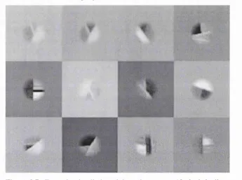
Figure 2.7 shows a number of real points of occlusion that are easily identifiable as such viewed
through apertures 13 pixels in diameter. All of these points generate local image structures that
we would be comfortable terming T-junctions.
Figure 2.7. Example stimuli viewed through apertures 13 pixels in diameter.
Even when only the local information visible through the apertures is
available, all of these locations are good candidates for occlusion points,
presumably because they generate T-junctions. Image is blown up for
reproduction purposes.
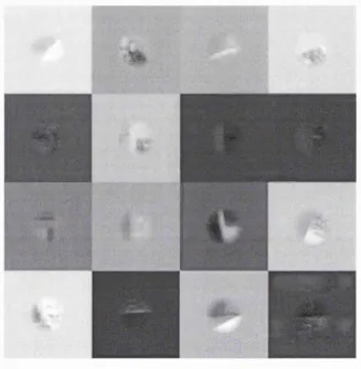
Figure 2.8 shows another group of occlusion points, again viewed through apertures 13 pixels in
diameter. In contrast to the previous group, none of these image patches are obviously the
product of an occlusion point, and accordingly none were correctly classified by our observers.
None of the occlusion points in this group generate prototypical T-junctions, for reasons that vary
from case to case. In some instances the occluded contour is very low contrast and hard to
... ..
ÎJS«’ =■ AïJfeÊrbs
QBUWB#
m m
Figure 2.8. Example stimuli stimuli viewed through apertures 13 pixels in
diameter. Just given the local evidence visible through these small apertures,
these locations are relatively poor candidates for occlusion points. Image is
blown up for reproduction purposes.
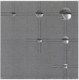
Figures 2.9-2.16 further illustrate this, showing some of these and other occlusion points over a
range of aperture sizes (the four smallest sizes used in the experiments). Although not obviously
occlusion points when viewed through the smallest apertures, as the aperture size increases it
becomes easy to tell that the image patches are centered on points of occlusion. In most of these
Figure 2.9. Example occlusion point viewed through apertures 13, 25, 49, and 97 pixels in
diameter. Location 14.
Figure 2.10. Location 114.
;
Figure 2.11. Location 153.
Figure 2.13. Location 165.
Figure 2.14. Location 186.
1
Figure 2.15. Location 203.
Figure 2.16. Location 215.
The fact that a large number of pixels (e.g. 50 by 50) is needed to recognize many points of
occlusion might indicate that a rather complicated mechanism is necessary for their detection
(more complicated than mechanisms that could detect synthetic junctions, which can evidently be
recognized with far less information). Before considering this possibility, however, we will first
2.4 Experiment 2: Controls W ith Zoomed Image Patches
One relatively uninteresting explanation of the basic result of Experiment 1 might involve lateral
masking between the aperture border and aspects of the image patch. For small apertures, the
borders are close to the center of the patch, and might thus interfere to a greater extent on
subjects’ ability to detect the image structure relevant to their occlusion judgments. It seemed
unlikely that masking could be so strong as to generate the trend present in our results, but we
nonetheless sought to rule it out. W e thus repeated Experiment 1 with the image patches "blown
up"; each image was upsampled and blurred to twice the original size.
Methods
Image patches were blown up by a factor of two using the upBlur function in Eero Simoncelli’s
M atlab Pyramid Toolbox. The patch sizes were 14, 26, 50, 98, and 194 pixels in diameter, each
generated from a patch of the original image half that size. Thus the smallest patch size was
generated from a patch 7 pixels in diameter, a size not included in the original experiment. The
other four patch sizes were generated from the four smallest sizes o f the original experiment.
Results
As shown in Figure 2.17, the basic result of Experiment 1 was replicated with the zoomed
patches; discrimination is poor for small apertures and improves markedly as the aperture size is
increased and a greater number o f pixels become visible. M oreover, the results were
quantitatively indistinguishable from those of Experiment 1 even though the displays were twice
as large and the aperture borders thus further from the relevant image structures. We wanted to
check if error rates were similar to those from the original experiment for patches generated from
the same number of pixels but displayed over a larger region, and the 95% confidence intervals,
plotted as error bars, confum that this is the case. There were no significant differences between
Figure 2.17. Error rates for different aperture sizes for zoomed stimuli. Error bars
denote 95% confidence intervals. Compare to Figure 2.4a.
Occlusion Classification of Zoomed Real Image Patches
Total Errors Results for 4 subjects
5^ 40
5 20
25 49
<—Patch Diameter in Pixels—>
We ran a second experiment on two subjects, in which the small patches were blown up more
than the large ones, such that the display size was the same for all the apertures. Again,
discrimination was much worse for the displays generated from a small number of pixels, even
though the patch borders were now at the same eccentricity in all conditions (data not shown). It
thus appears that interference by the aperture borders is unlikely to account for our results.
We also replicated the results of Experiment 1 with images reduced (blurred and subsampled) by
a factor of two. We took the labels of the original images and weeded out points that were no
longer visible in the reduced images (those that were formed by very thin contours in the original
images, for instance). We ran two subjects in the aperture size experiment with this new set of
locations from the reduced images, and found similar proportions of detectable occlusion points
for each patch size. This controls for the possibility that the CCD used to take the pictures might
have corrupted the high frequencies through aliasing. It also suggests that the image property we
are measuring in our experiments is statistically scale invariant, i.e. that the frequencies of
detectable occlusions at different aperture sizes are independent of the scale at which the image is
sampled. This is unsurprising given that the statistics of many image properties are scale
invariant in natural images (e.g. Ruderman and Bialek, 1994), but it confirms that pixels are the
right unit with which to measure the visual information used in our task (as opposed to, say,
In sum, it seems unlikely that our effects are due to problems with our stimuli. W hat else might
Chapter 3: Psychophysics Experiments on Scale
3.1 Experiment 3: Scale
Another obvious explanation of the results of Experiment 1 involves the spatial scale of any
putative signature of occlusion. Intensity changes in images due to object boundaries and other
structures in the world occur over both large and small scales (Koenderink, 1984), and one would
expect junctions to exist at different scales as well. The detection of junctions at large scales
would require analysis of a large image region even though they might require no more
parameters for their description than do fme-scale, locally defined junctions. As illustrated in
Figure 3.1, a large-scale junction lacking crisp edges is not clearly visible when viewed through a
small aperture - a large area is needed to detect the intensity gradients defining the junction.
Note, though, that this example junction is a simple structure and could presumably be recognized
with a fairly small number of image samples, they just need to be distributed over a large region
of space. Similar examples can be found in real images; Figure 3.2 shows one, and some of the
examples shown earlier also appear to fall in this category. Such image regions appear to contain
relatively simple image features even though they require a large area in order to be visible. The
dependence of occlusion detection on aperture size might thus be the result of simple image
structures distributed across a variety of scales, and could still be consistent with the notion of
junctions as simple and locally defined cues. It must be emphasized that this question, of whether
the existence of junctions at multiple scales can account for our results, is independent of our
observation that the dependence of occlusion detection on aperture size is scale invariant. It is
hard to see how the latter sort of scale invariance could fail to hold, since that would mean that
our results would be dependent on the distance from the scenes being imaged to the camera. The
present question, in contrast, is very much open and needs to be tested.
Figure 3.1. A blurred synthetic junction viewed through apertures 13, 25, 49, and 97 pixels in
% ** AS r«^rc*^3iv A i
Figure 3.2. An example real occlusion point which appears to have simple junction structure at a
large scale due to blurred edges. Location 760.
How can we test the extent to which large-scale junctions could account for our results?
Intuitively, we want to isolate the large-scale structure of image regions whose occlusion points
are not visible through small apertures, and see if the occlusion points remain detectable when
only the large-scale structure could be underlying performance. A standard technique for
isolating structure at large scales is to blur and subsample an image (e.g. Burt and Adelson,
1983). Blurring eliminates the fine scale structure, and subsampling converts the remaining low
frequencies into high frequencies defined over a small number of pixels. The point of this is
twofold. First, simply blurring the image patches would be confounded by the fact that the
resulting patches look blurry, which could conceivably affect subjects'judgments. Subsampling
the blurred patches makes them look as sharp as the originals. Second, the subsampling step
takes the large-scale structure that was formerly distributed over many pixels and compactly
represents it over a small set of pixels. If large-scale junctions are mediating occlusion
discrimination for the occlusion points that are visible only through large apertures, these points
should be rendered visible through small apertures once the large-scale structure is isolated via
blurring and subsampling. Figure 3.3 shows the effect of blurring and subsampling the large-
scale synthetic junction of Figure 3.1. Each row was generated by viewing a blurred and
subsampled version of the previous row’s image through apertures of different sizes. The
junction is not visible in the original image when viewed through the small aperture, but once
reduced it becomes crisp and easy to see. We thus have a test of the extent to which simple
Figure 3.3. Reduced versions of a blurred synthetic junction viewed through apertures of
different sizes. The image for each row is a reduced version of the previous rows image.
Note that the junction is visible in the reduced images viewed through the small
apertures, because the large scale structure defining the junction has been isolated.
Methods
Each image location was shown in 6 conditions: through (1) small, (2) medium, and (3) large
apertures at full resolution, (4) blurred, subsampled and viewed through a small aperture (i.e. the
medium apertures reduced once) and (5) blurred, subsampled and viewed through a medium
aperture (i.e. the large apertures reduced once), and (6) blurred and subsampled twice viewed
through small apertures (i.e. the large apertures reduced twice, down to the size of the small
apertures). The extent to which junctions at large scales might be mediating occlusion
discrimination can be measured by examining whether occlusion points that are visible through a
large aperture but not through a small one become visible through a small aperture once they have
been reduced.
Unlike the previous experiments, in which each image location was included in just a single
of the experiment’s design. This led to a concern that a subject’s judgm ent for a particular
location in one condition might influence their judgment for that location in another condition
seen later in the experiment. For an occlusion point clearly visible when viewed through a large
aperture, for instance, it seemed conceivable that when presented with the same image masked by
a smaller aperture subjects might realize that they had seen it before, and base their judgment on
having already seen it as an occlusion point regardless o f the local evidence for occlusion. To
minimize the chances of that sort of thing occurring, we randomly left-right reversed and rotated
the image patches 90 degrees clockwise or counter clockwise in the different conditions. This
made it less obvious that image patches were being shown multiple times. Subjects were not
informed that this was the case, and none ever reported seeing the same thing more than once; we
suspect the repeats had little to no effect on the results.
Subjects’ instructions were the same as in the previous two experiments. All subjects were naive
as to the specific purpose of this experiment. As in the previous experiments, feedback was given
to enable subjects to perform as well as possible.
W e ran two versions of the experiment, one in which the aperture sizes were 7, 13, and 25 pixels
in diameter and the images were expanded by a factor o f 2 as in Experiment 2, and one in which
the aperture sizes were 13, 25, and 49 pixels in diameter and the images were shown at full
resolution. Images were reduced by a factor of 2 or 4 in each dimension, and the aperture sizes
were chosen so that image patches visible through the larger apertures would reduce down to the
size o f the smaller apertures. Images were reduced (blurred and subsampled) using the blurDn
function in Eero Simoncelli’s Matlab Pyramid Toolbox. A 5-tap binomial filter was used for
blurring.
Results
To test for the presence of large-scale junctions, we examined all the points of occlusion which
were visible through large apertures but not through small apertures at normal resolution. Each of
Scale Analysis of Points of Occlusion
1-, (U H
c : 3 < C 100
(U
K
p <80
> tSJ) c ■£ e 00 o 601
40 Q C c/5 ooZ
c o 20 "u '•GCJu 3 0
o
13 DO C
Experiment A
Results for 4 subjectsvisible at 13 but not at 7
pixels
visible at 25 but not at 7
pixels
visible at 25 but not at 13
pixels
< t:
Experiment B
Results for 5 subjectsvisible at 25 but not at 13
pixels
visible at 49 but not at 13
pixels
visible at 49 but not at 25
pixels
Figure 3.4. Results of Experiment 3. Error bars are 95% confidence intervals.
Figure 3.4 plots the proportion of such occlusion points that remained visible after blurring and
subsampling, for each of the three analysis conditions in each of the two experiments. The results
of the two experiments are fairly similar: between 60 and 80 percent of the occlusion points that
subsampling, even though they are represented with far fewer pixels (1/4 or 1/16 as many,
depending on the analysis condition). This is good news for junction lovers, since it suggests that
in many cases in which occlusion points require a large region of analysis to be detected, there is
nonetheless a fairly simple signature of their presence.
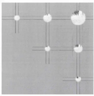
3.2 Scale Exam ples
Figures 3.5-3.10 show some examples for which this is clearly the case. As before, each row
consists of the same image viewed through apertures of different sizes. The image for each row
is a blurred and subsampled version of the image from the previous row. The aperture sizes are
arranged such that the image patches in each column cover the same region of the original image
at different scales. Occlusion is hard to see through the small apertures at high resolution, but is
much clearer after blurring and subsampling when the large-scale structure is isolated, mainly
because T-junctions become evident.
Figure 3.5. A real point of occlusion displayed at successively coarser scales, viewed
n - -s a r a '
i # sT#!
k; \ ;'.
m ^ m r
f
# 09%»^ ‘_* f A
Figure 3.6. Location 761.
:ïAë7.!:.j
m
:
Figure 3.8. Location 516.
«%
_____
N
■
Figure 3.10. Location 502.
lE .jgl' ,$%
,3 2r'S
I #'-T^:;: r ' W--
■'■ f i
:’
y * ^ ; y N *. I* V
0 9
9 0 JWKh*.*.However, upon inspection of other examples, it becomes clear that in some cases what appears to
be evidence for occlusion after blurring and subsampling is in some sense artifactual.
Figure 3.13. Example of an occlusion point that is artifactually visible given local
information at a large scale. See text for details. Location 702.
Figure 3.13 shows one such example. The contour being occluded at the center of the patch is the
edge of a tree trunk which happens to be fairly low contrast and in part visible due to a texture
boundary. It is not visible until a large region is available for analysis. When the image is
reduced, the vertical edge of the labeled occlusion point becomes invisible, but the shading on the
tree trunk produces a high contrast edge that is shifted towards the center of the patch by the
reduction process. This image was classified as an occlusion point, but the T-junction responsible
for the judgment is not the product of the occlusion point under consideration, and is not even
produced by something that was labeled as an occlusion point in the original image. The fact that
subjects make the correct response for a stimulus such as this is thus an artifact of the reduction
process. The response is artifactual in the sense that the apparent large-scale signature of
in the world that was originally labeled, either being due to another nearby occlusion point
brought closer to the center of the image by the reduction process, or an accidental large-scale
image structure, and 2) presumably not responsible for the (correct) percept of occlusion in the
full-scale patches.
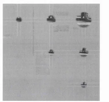
3.3 Scale Artifacts
W e are thus probably overestimating the extent to which occlusion points are often indicated by
large-scale occlusion cues; some of what appear to be occlusion cues are artifacts. Fortunately,
we can estimate the frequency with which these artifactual occlusion signatures are produced by
examining our subjects’ occlusion judgments on the randomly selected patches. W e looked at
those randomly selected patches which were correctly labeled as not being occlusion points at
two aperture sizes, and computed the proportion which were then labeled (incorrectly) as
occlusion points when they were reduced from the size of the large aperture to that of the small
one. Since these points were originally selected at random and did not appear to be occlusion
points at either aperture size at full resolution, we can be reasonably sure that the appearance of
occlusion in the reduced image is an artifact of the reduction. M oreover, the appearance of
occlusion in the reduced image clearly is not the determinant o f occlusion judgments for the full
resolution images, because we have selected patches that at full resolution are judged to not be
occlusion points. One might thus say that the large-scale structure at such points is both
physically artifactual (in that they are not really due to an occlusion point at the center of the
patch) and psychologically artifactual (in that they are not responsible for occlusion percepts at
full resolution). Figures 3.14-3.17 show several examples of image patches from our randomly
I
Figure 3.14. Example of a randomly selected patch which at large scales
^ â
m m
9
=
0#0BM S P
m m »
##
#m
dmwMN
T.
#P
Figure 3.16. Additional example of an artifactual large-scale occlusion signature.
1#
Figure 3.17. Additional example of an artifactual large-scale occlusion
signature.
Figure 3.18 plots the proportion of these artifactual occlusion judgments for each of the three
analysis conditions in each experiment. On average, blurring and subsampling introduces
artifactual occlusion signatures in around 20 percent of the randomly selected patches. Assuming
that the frequency of these artifacts is the same for image regions centered on actual points of
occlusion and those randomly selected, we can estimate that on the order of 20 percent of the
occlusion points visible after blurring and subsampling are artifactual: the large-scale structure,
although apparently consistent with occlusion, is neither physically due to occlusion nor
psychologically responsible for occlusion judgments at full resolution. The proportion of
Artifactual Large-scale Occlusion Signatures
Experiment A
Results for 4 subjects§ C o 100 u o
o
'- B c o U 80 60 > '.n CL o 40Oh c(U
M £ c3 20 ~o 3 •—> 0 correctly rejected at both 13 and 7
pixels
correctly rejected at both 25 and 7
pixels
correctly rejected at both
25 and 13 pixels
Experiment B
Results for 5 subjects1 1
II
P
il
tin -3^100 80 60 40 20
_ É _
correctly correctly correctly rejected at both rejected at both rejected at both
25 and 13 49 and 13 49 and 25
pixels pixels pixels
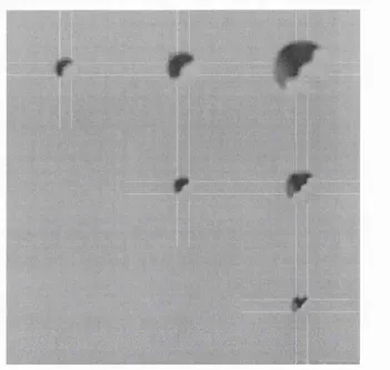
3.4 Nonlocally Defined Occlusion Points
Figures 3.19-3.24 show several examples which fall in this category; these occlusion points do
not become visible until viewed through large apertures, and blurring and subsampling them does
not preserve this visibility. This is for a variety of reasons. In some cases one or more of the
contours is not visible at the larger scales (because lines, unlike step edges, are not scale
invariant); in other cases spurious large-scale structures are introduced which seem inconsistent
with occlusion. Perhaps a quarter of our occlusion points fall in this category; their detection
evidently requires a mechanism that can make use of all of the pixels in a large region.
F C" , ■ .
Figure 3.19. Example of an occlusion point whose visibility requires a large number of pixels
regardless of the scale of analysis. Here the stem of the junction is a thin contour that is
Figure 3.20. Another example of an occlusion point whose
visibility requires a large number of pixels regardless of the
Figure 3.21. Another such example, with four aperture sizes instead of three. Here the branches
are difficult to individuate for all but the largest apertures.
A
, ^ S'
Figure 3.22. Another example. The structure of the woman’s shirt sleeve near the occlusion
Figure 3.23. Here the thin stem contour is again lost at large scales and hardly present locally.
3.5 Scale Selection
But although many occlusion points seem to necessitate analysis of fine scale structure over a
large region, a substantial portion produce fairly simple signatures that are visible at fine scale,
and the remainder seem to produce fairly simple signatures only at a large-scale. If there was a
simple way to select the scale of analysis, a large proportion of occlusion points could thus be
detected using fairly simple mechanisms. The selection of the correct scale is critical, though.
The existence of artifactual junctions at large scales discussed earlier implies that one cannot
simply take a junction at a large-scale as evidence for occlusion; large-scale structures are
frequently spurious. Moreover, spurious large-scale structure generally does not "fool" the
human visual system, implying that scale selection mechanisms are at work in human vision.
W hat might they involve?
M any theories of scale selection rely on the magnitude of image gradients at different scales to
choose the scale of analysis. Elder and Zucker (1998), for instance, have proposed an elegant
framework that chooses the minimum reliable scale for edge detection by comparing gradient
magnitudes at different scales with the values that would be produced by sensor noise alone (see
also Morrone, Navangione, and Burr, 1995; Lindeberg, 1996). Edge detection at a particular
location is conducted at the minimum scale where the gradient exceeds these noise levels. This
prevents spurious responses to noise (to which fine scale operators are more vulnerable) while
minimizing the interference of neighboring image structure (which is a problem at large scales, as
we have seen). One could envision a similar scheme for junction detection at different scales;
detection would occur at the minimum scale at which the gradient magnitudes exceeded the levels
expected just from noise.
For some junctions, such a strategy seems reasonable. Consider, for instance, the blurry synthetic
junction of Figure 3.1 that was used as a motivating example: there is very little high frequency
structure. W hen viewed through a small aperture at high resolution, little is visible other than a
few blurry image gradients, if that. Derivative magnitudes computed for this junction will be
the pole that has an unusual shape due to the pole’s curvature. When viewed through a small
aperture, the shadow is hard to interpret as such and prevents most observers from correctly
categorizing the image as an occlusion point. When observers have access to a larger region of
the image, the shape of the pole becomes evident and the shadow starts to look like a shadow, and
it becomes obvious that there is a point of occlusion at the center of the image. Notably, most
observers continue to classify this image as an occlusion point after it is reduced. This is because
the reduction erases the small shadow, leaving what appears to be a fairly crisp T-junction.
However, the high frequency structure in the image is salient and inconsistent with the large-scale
T-junction. The scale selection methods outlined above would clearly fail to isolate the large-
scale structure in images such as this - there is abundant high contrast, high frequency structure,
and no obvious bottom-up method with which to select the large-scale for junction analysis. We
cannot directly estimate the frequency of this situation from our data, but inspection of our stimuli
suggests that it is quite common.
Figure 3.25. Example of an occlusion point where a cast shadow drastically alters the
local intensity signature. Although there is a junction at coarse scales, how should one
choose to ignore the fine scale shadow unless it has already been recognized as such?
Thus even though points of occlusion in many cases generate large-scale junctions, the utility of
selecting the proper scale of analysis. If scale is not properly selected, false positive responses to
spurious large-scale structure will result. In many cases, it is not obvious that there is a bottom-
up method for scale selection (e.g. in our shadow example), in which case the presence of large-
scale junctions does not simplify the analysis of the large pixel arrays needed to detect many of
our points of occlusion. In our shadow example, the shadow may need to be recognized as a
shadow before occlusion can be identified.
The shadow example also highlights a shortcoming of our paradigm, namely that it is difficult to
say anything specific about why so many pixels are needed to detect certain points of occlusion.
The fact that observers require a large number of pixels is consistent with both bottom-up (low
contrast contours must be integrated across large numbers o f pixels to be detectable, textures
require large numbers o f pixels to be segregated, etc.) and top-down (shadows must be correctly
interpreted) accounts of how occlusion points are being detected. For individual examples, we
can speculate what is going on, but it is not obvious how to assess this issue experimentally
across an ensemble o f occlusion points. For shadows, presenting the images in negative might be
an effective way of testing how often shadow interpretation is critical to detecting occlusion
points, since shadows are generally interpreted as such only when they are dark (Cavanagh and
Leclerc, 1989; Anstis, 1992), but in general we lack a method to assess the importance of high
level interpretation.
3.6 General Discussion of Psychophysics
We have introduced a method for studying local occlusion cues in real images. Our results offer
some new insights into junctions and their detection that would be difficult to obtain with
traditional psychophysics experiments using synthetic stimuli, because synthetic stimuli do not
reflect the demands of the real world. Our results suggest that although junctions as traditionally
conceived do indeed occur at a significant number of occlusion points in real images, many other
occlusion points lack a simple, local signature. The recovery o f occlusion geometry may thus
stimuli are poorly controlled and the judgments ill-defined in comparison to traditional
psychophysics with synthetic stimuli. W e think that in many instances these difficulties are not
insuperable, in which case our approach may be a useful addition to the vision scientist’s toolbox.
Nonetheless, there are a number of potential concerns with our paradigm that we wish to address.
First, the success of our method depends critically on the ability o f observers to perform the task
effectively. One might argue that people simply might not know what characterizes occlusion
points in real images, since they are not used to seeing them in isolation. Perhaps as a result of
this they might be impaired at our task irrespective o f the available local information. This is a
possibility we can never fully rule out, but we did take a num ber of steps to minimize the chances
of this. Stimulus duration was unlimited, and subjects were encouraged to take as long as they
needed on each trial. The responses to our synthetic junctions inserted as catch trials helped to
insure that subjects were doing something reasonable. Inspection of their responses to various
stimuli further confirm this. Furthermore, our subjects received feedback on their responses and
were instructed to use the feedback to maximize their performance. Subjects were initially given
extensive practice prior to taking part in the actual experiments, and most o f our subjects came
back for multiple sessions. Subjects did improve somewhat with practice, but even our most
practiced subjects were unable to make fewer than 20 percent errors in classifying real image
patches through the smallest apertures we used. In addition, the task we required subjects to
perform was both natural to our subjects and of obvious ecological relevance. Given all this, it
seems likely that our subjects were fairly effective at picking out local occlusion cues when they
were present.
A second area of concern is the choice of randomly selected image patches as negative examples
o f points of occlusion. The negative examples are critical to investigating occlusion detection,
since otherwise subjects could simply label everything a point of occlusion without even looking
at the stimuli. Given that we are interested in how occlusion points might be detected in real
images, patches of real images not centered on occlusion points seemed the logical thing to use as
negative examples. As we have discussed, many randomly selected patches of real images are
fairly uniform at the center, and thus trivially easy to distinguish from a likely point of occlusion.
To force subjects to make a more specific discrimination, we screened out those randomly
selected patches whose intensity variance was below a threshold and added synthetic edges as
additional negative examples, but these were essentially arbitrary steps. The negative examples
make an even more specific judgment, and only label points of occlusion as such if they are
signified by very well-defined junctions.
A third concern, also alluded to earlier, is also related to the negative examples. A consequence
of using randomly selected image patches as the negative examples is that some fraction of them
were actually points o f occlusion. The presence of these impostor stimuli results in inflated false
positive levels; many o f the false positive errors subjects make are not really errors. Again, a
more carefully chosen set of negative examples could avoid this problem.
Addressing each of these issues differently could certainly alter our quantitative results to some
degree, but it seems unlikely that our qualitative conclusions would be substantially affected. We
are hopeful that such concerns could be dealt with in other contexts as well.
Although our methodology could conceivably be applied to a variety o f topics in early vision, it
could also be used to further investigate occlusion detection in human vision. Our results with
synthetic junctions suggest that our paradigm can be used to measure the extent to which any
arbitrary synthetic stimulus is interpreted as being due to occlusion. W e found that when
intermixed with real image patches, our synthetic T-junctions were nearly always judged to be
points of occlusion whereas our synthetic L-j unctions were not. This is consistent with other
psychophysical results on the interpretation of isolated junctions (McDermott and Adelson,
unpublished manuscript). This suggests an attractive method for investigating other stimulus
properties potentially related to occlusion. Synthetic stimuli could be generated that vary along
dimensions of interest, and inserted alongside the real image patches in an experiment similar to
those we have described. The extent to which they are judged to be occlusion points can be taken
as a measure of the strength of the occlusion cue being manipulated. For instance, Stevens and
Brookes (1988) have proposed that concave cusps offer a strong cue to occlusion, and constructed
a number of complicated displays as evidence for this. One could perhaps better isolate the effect
by incorporating concave cusps into an occlusion detection experiment with real images. With
larger displays one could also conceivably study the influence of context on the interpretation of
enhance even the local sense of depth and three-dimensionality, which in turn can greatly
strengthen the percept o f occlusion. Contour curvature also made a substantial contribution.
M any junctions formed by straight edges with sectors of uniform luminance convey very weak
percepts of occlusion, presumably because they have other plausible explanations. These
observations are informal, but suggest that there may be a rich assortment o f local occlusion cues
that could be studied in the manner we have discussed.
W e can draw a number of conclusions from the experiments described so far. First, we have
addressed the question of whether junctions are in fact locally defined. It appears that although a
fraction of junctions are indeed detectable given purely local information, many others require
larger image regions in order to be seen. Many junctions do not become visible until the image
region containing them is sufficiently large that many other things are visible besides just the
junction: other edges, other junctions, patches of texture etc. Moreover, often this is not simply a
matter of selecting the correct scale of analysis, a large num ber o f pixels are needed to detect
many junctions even at the appropriate scale. This suggests that any mechanisms for detecting
junctions are performing a nontrivial analysis of a high dimensional input space. The negative
spin on these results is that junctions may not be all they are cracked up to be - a significant
fraction are not locally detectable, and thus may not be good candidates for foundational elements
o f vision. The flip side to this, though, is that a significant fraction of junctions are locally
detectable. This means that local mechanisms, operating on image regions on the order of 10-15
pixels in diameter, ought to be able to detect this portion of the things that people label as
junctions when viewing the whole image. We therefore attempted to learn to detect junctions
Chapter 4: Neural Networks for Junction Detection
4.1 General Motivation
First of all, why should one try to build a junction detector? W e had several motivations. First, a
functioning junction detector would be useful for a variety o f image interpretation tasks, and
particularly for object recognition algorithms which depend on the shape o f the bounding contour.
Second, a functioning junction detector which operates on local image regions could further
corroborate our psychophysics results showing that many junctions are locally defined and could
play an early role in human vision. Third, the way that a working junction detector works might
provide clues to how the brain might solve the same problem.
Our main motivation, though, was that a functioning junction detector, regardless of its biological
plausability, would be useful for measuring junction statistics. O f primary interest are the
probabilities with which junctions are actually associated with the scene events like occlusion to
which they are purported to be cues. Figure 4.1 shows an image o f a zebra whose stripes produce
a host of T-junctions. Notably, though, nearly all of them DO NOT indicate occlusion. T-
junctions like these, that are not due to occlusion, are easy to find once you start looking for them.
It remains unclear just how common they are relative to the generic type caused by occlusion.
W ithout a principled method of systematically finding junctions, we lack a good method with
which to measure the frequencies of generic and non-generic T-junctions and thus measure the
extent to which T-junctions are in fact good cues. Assuming one could produce a mechanism
capable of labeling local T-junctions with reasonable accuracy, one could then scan it across a
collection of images and check the degree of correspondence between points of occlusion and T-
junctions. To be able to do this, and hence compute the cue probability, would be of substantial
^ ___
Figure 4.1. A zebra, which generates a host of T-junctions nearly all of which are
inconsistent with the border ownership
There are thus a number of reasons to try to produce a good junction detector. Unfortunately, this
is easier said than done. Previous attempts to detect junctions have mostly been "top-down":
people have started with some idea of what is appropriate, and then tried to make it work.