Visualization of Performance of Interpolation Search in Worst Case in Personal Computer using Polynomial Curve Fitting

(1)

Volume 8, No. 1, Jan-Feb 2017

International Journal of Advanced Research in Computer Science

RESEARCH PAPER

Available Online at www.ijarcs.info

Visualization of Performance of Interpolation Search in Worst Case in Personal

Computer using Polynomial Curve Fitting

Dipankar Das

Abstract: It is a well known fact that, in this modern era, the data visualization has become very important in almost all the areas of human life including science and technology. In this paper, we have made an attempt to visualize the behaviour of interpolation search by measuring its time in worst case for a varying size of equi – interval sets of data in a personal computer (desktop) using polynomial curve fitting technique. It has been observed that in the worst case this search technique behaviourally does not fit to any particular polynomial model i.e. polynomial model of a particular degree for the varying size of equi – interval sets of data. In this paper, the researchers have also shown the smooth spline curves passing through the predicted values obtained by using the best fit polynomial models for the varying size of equi – interval sets of data.

Keywords: Interpolation search; Polynomial curve fitting; AIC; BIC; spline

I. INTRODUCTION

A search technique in computer science is an attempt to retrieve information from a list of items, which is often represented by some data structure i.e. Arrays, Lists etc. Over a period of time many search algorithms came into existence each with its wide acceptance and uber goal, the two most popular search techniques to start with are linear search and binary search, but some other search techniques like Fibonacci search for finding the maximum of a unimodal function, exponential search, hash technique gained wide importance too. In this paper we tried to analyze the time performance of Interpolation search which is a slight modification of binary search where we need one additional information about data to speed up the search process, we are considering Interpolation search over Binary search where theoretical time complexity adapting big-O notation on n elements is O(n); if the data is uniformly distributed linearly for interpolation, the performance is O(log log n) whereas in case of binary search on the data set of size n, the time performance is O(log n).

In this research, we tried to analyze and visualize the time performance of Interpolation search on the fly (in the worst case) using polynomial curve fitting technique to depict which polynomial curve fits best to the performance of Interpolation search, however in order to achieve we just kept things simple without consideration of the factors i.e. context switching, buffer, cache management etc which we believe also plays key role in time performance of this search technique and will provide new avenues to carry our research further in time to come.

II. LITERATURE REVIEW

Gonnet, Rogers & George (1980) had given a brief survey of interpolation search algorithm and analyzed the complexity

of the search method [8]. Carlsson & Mattsson (1988) in their work had presented improvements of interpolation search [6]. Marsaglia & Narasimhan (1993) had designed an efficient algorithm for simulating an interpolation search by using simple results in mathematical statistics [4]. Demaine, Jones &

Pătraşcu (2004) in their work had captured the pseudo

randomness of interpolation search [5]. Kaporis et al. (2006) had presented a new dynamic interpolation search technique which had obtained O(log log n) search time [7]. Roy & Kundu (2014) had done a comparative analysis of linear, binary and interpolation search [9]. Verma & Paithankar (2016) had implemented interpolation search technique with memorization and observed a significant time reduction [10].

III. OBJECTIVES OF THE STUDY

• To identify the best polynomial models that can be fitted to the data points (execution time in seconds versus data size) for interpolation search in the worst case executed in a personal computer (desktop) for different data sizes

• To visualize the best polynomial models that can be fitted to the data points (execution time in seconds versus data size) for interpolation search in the worst case executed in a personal computer (desktop) for different data sizes

IV. METHODOLOGY

(2)

• Data size twenty five (25) to one hundred five (105) with an interval of five (5)

• Data size one hundred forty (140) to three hundred (300) with an interval of ten (10)

• Data size seven hundred (700) to two thousand three hundred (2300) with an interval of one hundred (100) • Data size four thousand (4000) to twelve thousand

(12000) with an interval of one thousand (1000) • Data size fifty one thousand (51000) to two hundred

thirty one thousand (231000) with an interval of ten thousand (10000)

For each of the observations we have collected seventeen (17) data points.

The researchers have used curve fitting technique to identify the best polynomial curve that can be fitted to the different set of observations (execution time in seconds versus data size). In total, we have used ten (10) numbers of models, polynomial of degree one i.e. linear to polynomial of degree ten models to identify the best curves that can be fitted to the different set of observations (execution time in seconds versus data size). For identifying the competing models we have considered R square, Adjusted R square and Root Mean Square Error (RMSE) as goodness of fit measures. The decision rule for identifying the competing model is to have high value (value close to one) of R square and Adjusted R square and low value (value close to zero) of RMSE [1]. The best curve amongst the competing curves is identified by using Akaike information criterion (AIC) and Bayesian information criterion (BIC). These two different information criteria may provide us two different models for the same data set. The decision rule is as follows: the model which is having lowest AIC value is selected [2][3] and the model which is having lowest BIC value is selected [3].

The hardware configuration of the personal computer (desktop) under study is as follows:

• Processor: Intel(R) Core(TM) i3-6100 CPU @ 3.70GHz

• Memory: 4096MB RAM

The software used for data analysis: R version 3.3.1 (2016-06-21)

V. DATA ANALYSIS &FINDINGS

The R square, Adjusted R square and Root Mean Square Error (RMSE) of different polynomial models tried on the data points (execution time in seconds versus data size) for interpolation search in the worst case executed in a personal computer (desktop) for data size twenty five (25) to one hundred five (105) with an interval of five (5) is given in the following table (Table I):

Table I. R Square, Adjusted R Square & RMSE of The Polynomial Models for Data Size Twenty Five (25) to One Hundred Five (105) with an Interval of

Five (5)

Model Name R Square Adjusted R Square RMSE

Polynomial of degree 1 0.0005636 -0.06607 1.74243

Polynomial of degree 2 0.3187 0.2214 1.438609

Findings: From the above table (Table I) we have identified the following four (4) models as the competing models:

Polynomial of degree 7, Polynomial of degree 8, Polynomial of degree 9 & Polynomial of degree 10.

The AIC and BIC values of the above four competing models are given in the following table (Table II).

Table II. AIC & BIC of The Competing Polynomial Models for Data Size Twenty Five (25) to One Hundred Five (105) with an Interval of Five (5)

Model Name AIC BIC

Polynomial of degree 7 55.29719 62.79611 Polynomial of degree 8 54.15247 62.4846 Polynomial of degree 9 54.7735 63.93884 Polynomial of degree 10 54.41117 64.40973

Findings: From the above table (Table II) we observe that the “polynomial of degree 8” model has lowest AIC & BIC values. Therefore, this polynomial model fits this set of data well.

The R square, Adjusted R square and Root Mean Square Error (RMSE) of different polynomial models tried on the data points (execution time in seconds versus data size) for interpolation search in the worst case executed in a personal computer (desktop) for data size one hundred forty (140) to three hundred (300) with an interval of ten (10) is given in the following table (Table III):

Table III. R Square, Adjusted R Square & RMSE of The Polynomial Models for Data Size One Hundred Forty (140) to Three Hundred (300) with an

Interval of Ten (10)

Findings: From the above table (Table III) we have identified the following two (2) models as the competing models: Polynomial of degree 9 & Polynomial of degree 10.

The AIC and BIC values of the above two competing models are given in the following table (Table IV).

Table IV. AIC & BIC of The Competing Polynomial Models for Data Size One Hundred Forty (140) to Three Hundred (300) with an Interval of Ten (10)

Polynomial of degree 9 86.239 95.4044 Polynomial of degree 10 87.4145 97.4131

Findings: From the above table (Table IV) we observe that the “polynomial of degree 9” model has lowest AIC & BIC values. Therefore, this polynomial model fits this set of data well.

The R square, Adjusted R square and Root Mean Square Error (RMSE) of different polynomial models tried on the data points (execution time in seconds versus data size) for interpolation search in the worst case executed in a personal computer (desktop) for data size seven hundred (700) to two thousand three hundred (2300) with an interval of one hundred (100) is given in the following table (Table V):

Table V. R Square, Adjusted R Square & RMSE of The Polynomial Models for Data Size Seven Hundred (700) to Two Thousand Three Hundred (2300)

with an Interval of One Hundred (100)

(3)

Findings: From the above table (Table V) we cannot identify any model as the competing model because all the models are having negative Adjusted R square value.

The R square, Adjusted R square and Root Mean Square Error (RMSE) of different polynomial models tried on the data points (execution time in seconds versus data size) for interpolation search in the worst case executed in a personal computer (desktop) for data size four thousand (4000) to twelve thousand (12000) with an interval of one thousand (1000) is given in the following table (Table VI):

Table VI. R Square, Adjusted R Square & RMSE of The Polynomial Models for Data Size Four Thousand (4000) to Twelve Thousand (12000) with an

Interval of One Thousand (1000)

Findings: From the above table (Table VI) we have identified the following four (4) models as the competing models: Polynomial of degree 7, Polynomial of degree 8, Polynomial of degree 9 & Polynomial of degree 10.

The AIC and BIC values of the above two competing models are given in the following table (Table VII).

Table VII. AIC & BIC of The Competing Polynomial Models for Data Size Four Thousand (4000) to Twelve Thousand (12000) with an Interval of One

Thousand (1000)

Polynomial of degree 7 93.23474 100.7337 Polynomial of degree 8 94.6053 102.9374 Polynomial of degree 9 96.58062 105.746 Polynomial of degree 10 94.18913 104.1877

From

the above table (Table VII) we observe that the “polynomial of degree 7” model has lowest AIC & BIC values. Therefore, this polynomial model fits this set of data well.

The R square, Adjusted R square and Root Mean Square Error (RMSE) of different polynomial models tried on the data points (execution time in seconds versus data size) for interpolation search in the worst case executed in a personal computer (desktop) for data size fifty one thousand (51000) to two hundred thirty one thousand (231000) with an interval of ten thousand (10000) is given in the following table (Table VIII):

Table VIII. R Square, Adjusted R Square & RMSE of The Polynomial Models for Data Size Fifty One Thousand (51000) to Two Hundred Thirty

One Thousand (231000) with an Interval Of Ten Thousand (10000)

Findings: From the above table (Table VIII) we have identified the following three (3) models as the competing models: Polynomial of degree 8, Polynomial of degree 9 & Polynomial of degree 10.

The AIC and BIC values of the above two competing models are given in the following table (Table IX).

Table IX. AIC & BIC of The Competing Polynomial Models for Data Size Fifty One Thousand (51000) to Two Hundred Thirty One Thousand (231000)

with an Interval of Ten Thousand (10000)

Polynomial of degree 8 75.55509 83.88722 Polynomial of degree 9 72.18887 81.35422 Polynomial of degree 10 74.01881 84.01737

From the above table (Table IX) we observe that the “polynomial of degree 9” model has lowest AIC & BIC values. Therefore, this polynomial model fits this set of data well.

VI. CONCLUSION

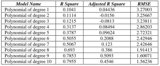
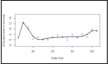
From the above analysis we have observed that for first data set (D1) i.e. data size twenty five (25) to one hundred five (105) with an interval of five (5) “polynomial of degree 8” model, for second data set (D2) i.e. data size one hundred forty (140) to three hundred (300) with an interval of ten (10) “polynomial of degree 9” model, for third data set (D3) i.e. data size seven hundred (700) to two thousand three hundred (2300) with an interval of one hundred (100) no model, for fourth data set (D4) i.e. data size four thousand (4000) to twelve thousand (12000) with an interval of one thousand (1000) “polynomial of degree 7” model and for fifth data set (D5) i.e. fifty one thousand (51000) to two hundred thirty one thousand (231000) with an interval of ten thousand (10000) “polynomial of degree 9” model fit the data well. The visualizations of these are given below. The black circles indicate observed data points, the red circles indicate predicted data points and the blue lines indicate the polynomial models.

(4)

Figure 2. Polynomial of degree 9 model for data set D2

Figure 3. Scatter plot for data set D3

From the above tables & figures we observe that excluding the data set D3 (i.e. data size seven hundred (700) to two thousand three hundred (2300) with an interval of one hundred (100)) all the data set (D1, D2, D4 & D5) can be fitted with higher order polynomial models. The polynomial of degree 9 fits the data set D2 and D5 whereas the polynomial of degree 8 fits the data set D1 and the polynomial of degree 7 fits the data set D4. Therefore, we observe that though four data sets (4) out of five (5) can be fitted to the higher order polynomials but all of them cannot be best fitted with the same degree of polynomial. In this study, the researchers have tried to visualize

the performance of the interpolation search in the worst case observed in a personal computer (Desktop) using polynomial curve fitting technique. We have limited our study up to polynomial of degree 10 and our conclusions are based on these observations only. The smooth curves going through the data points obtained from the best fitted polynomial models (i.e. predicted values) using splines are shown in the following figures:

Figure 6. Smooth spline curve passing through the data points (predicted values) using Polynomial of degree 8 model for data set D1

(5)

VII. REFERENCES

[1] Fit. (n.d.). Retrieved January 10, 2017, from

https://in.mathworks.com/help/curvefit/evaluating-goodness-of-fit.html

[2] MAZEROLLE, M. J. (n.d.). APPENDIX 1: Making sense out of Akaike’s Information Criterion (AIC): It...and interpretation in model selection and inference from ecological data [PDF]. Retrieved January 10, 2017, from http://avesbiodiv.mncn.csic.es/estadistica/senseaic.pdf [3] Maydeu-Olivares, A., & Garcı ́ a-Forero, C. (2010).

Goodness-of-Fit Testing [PDF]. Elsevier Ltd. Retrieved

January 10, 2017, from http://www.ub.edu/gdne/amaydeusp_archivos/encycloped

ia_of_education10.pdf

[4] Marsaglia, G., & Narasimhan, B. (1993). Simulating interpolation search. Computers & Mathematics with Applications, 26(8), 31-42. Retrieved February 6, 2017 from

http://www.sciencedirect.com/science/article/pii/0898122 19390329T

[5] Demaine, E. D., Jones, T., & Pătraşcu, M. (2004, January). Interpolation search for non-independent data. In Proceedings of the fifteenth annual ACM-SIAM symposium on Discrete algorithms (pp. 529-530). Society for Industrial and Applied Mathematics. Retrieved

February 6, 2017 from http://dl.acm.org/citation.cfm?id=982870

[6] Carlsson, S., & Mattsson, C. (1988). An extrapolation on the interpolation search. SWAT 88 Lecture Notes in Computer Science, 24-33. doi:10.1007/3-540-19487-8_3 [7] Kaporis, A., Makris, C., Sioutas, S., Tsakalidis, A.,

Tsichlas, K., & Zaroliagis, C. (2006, July). Dynamic interpolation search revisited. In International Colloquium on Automata, Languages, and Programming (pp. 382-394). Springer Berlin Heidelberg. Retrieved February 6,

2017 from http://link.springer.com/chapter/10.1007/11786986_34

[8] Gonnet, G. H., Rogers, L. D., & George, J. A. (1980). An algorithmic and complexity analysis of interpolation search. Acta Informatica, 13(1), 39-52. doi:10.1007/bf00288534

[9] Roy, D., & Kundu, A. (2014). A Comparative Analysis of Three Different Types of Searching Algorithms in Data Structure. International Journal of Advanced Research in Computer and Communication Engineering, 3(5), 6626-6630. Retrieved February 06, 2017, from http://ijarcce.com/upload/2014/may/IJARCCE6C%20a%2 0arnab%20A%20Comparative%20Analysis%20of%20Th ree.pdf

[10] Verma, D., & Paithankar, K., Dr. (2016).