Equivalent Damping in Support of Direct Displacement-Based Design with Applications to Multi-Span Bridges

ABSTRACT

DWAIRI, HAZIM M. Equivalent Damping in Support of Direct Displacement-Based Design with Applications to Multi-Span Bridges. (Under the direction of Dr. Mervyn Kowalsky.)

t

BIOGRAPHY

Hazim Dwairi was born in 1974 in Irbid city, Jordan. He joined the Civil Engineering Department at Jordan University of Science and Technology (JUST), Jordan, and earned his Bachelor degree in 1997. Afterwards, he joined the graduate school at JUST to earn his Master of Science degree in Structural Engineering in 1999. He worked for 2 years after that as a design engineer, designing various reinforced concrete structures. He came to Raleigh, North Carolina in August 2001 and joined the Civil Engineering Ph.D. program at North Carolina State University (NCSU). At NCSU, Hazim met Mervyn Kowalsky, who focused his attention to earthquake engineering and introduced him to the state of the art in that field. Hazim’s research interests include but not limited to seismic analysis and design of structures, laboratory testing of reinforced and prestressed concrete members, and on site testing of highway bridges. Hazim completed his Ph.D. degree in December 2004 and he is expected to join the Civil Engineering Department at Hashemite University (HU), Zarqa, Jordan as a faculty member.

Hazim M. Dwairi Raleigh, Nor h Carolina

December 2004

ACKNOWLEDGMENTS

The author would like to express his sincere thanks and gratitude to the following:

• Allah, for giving me the ability to think as well as the health and the patience to complete this work.

• My family, whom without their support, encouragement, and motivation, this work would not have been possible.

• My advisor, Dr. Mervyn Kowalsky, for his continuing technical and moral support over the course of the past three years. I thank Dr. Kowalsky for his generosity in passing on his knowledge to me, and for finding the time and patience to discuss my ideas.

• My advisory committee members: Dr. James Nau, Dr. Paul Zia, Dr. Vernon Matzen and Dr. Robert Bardon for their help and guidance.

• Dr. Eduardo Miranda, Stanford University, California, for providing us with a catalogue of one hundred earthquake motions.

TABLE OF CONTENTS

LIST OF TABLES ...VI

LIST OF FIGURES ...VIII

LIST OF ABBREVIATIONS AND SYMBOLS ... XII

PART I: INTRODUCTION AND RESEARCH OBJECTIVES... 1

1. INTRODUCTION...2

2. DISSERTATION ORGANIZATION...3

3. FORCE-BASED SEISMIC DESIGN...4

4. FUNDAMENTALS OF DIRECT DISPLACEMENT-BASED DESIGN...7

5. DESIGN LIMIT STATES...9

6. EQUIVALENT DAMPING APPROACH...13

7. RESEARCH OBJECTIVES...20

8. REFERENCES...21

PART II: ... 23

EQUIVALENT DAMPING IN SUPPORT OF DIRECT DISPLACEMENT- BASED DESIGN 1. INTRODUCTION...25

2. PAPER LAYOUT...27

3. JACOBSEN’S EQUIVALENT DAMPING APPROACH...27

4. REVIEW OF DIRECT DISPLACEMENT-BASED DESIGN...29

5. EVALUATION PROCEDURE AND RESUTS...31

6. EQUIVALENT DAMPING MODIFICATION...42

7. CONCLUSIONS...46

8. REFERENCES...48

PART III: ... 51

INELASTIC DISPLACEMENT PATTERNS IN SUPPORT OF DIRECT DISPLACEMENT-BASED DESIGN FOR CONTINUOUS BRIDGE STRUCTURES 1. INTRODUCTION...53

2. EVALUATION OF INELASTIC DISPLACEMENT PATTERNS...55

3. DDBD PROCEDURE FOR MULTI-SPAN BRIDGE STRUCTURES...64

4. SAMPLE BRIDGE DESIGNS...70

5. EVALUATION OF DDBD FOR MULTI-SPAN BRIDGES...83

6. CONCLUSIONS...86

PART IV: SUMMARY AND CONCLUSIONS... 90

1. CONCLUSIONS...91

2. RECOMMENDATIONS...94

3. FUTURE WORK...95

APPENDIX A: ... 97

SINUSOIDAL MOTIONS AND SOIL TYPE EFFECTS ON EQUIVALENT DAMPING A1. INTRODUCTION...98

A2. SINUSOIDAL EXCITATION RESULTS...98

A3. SOIL TYPE EFFECT...101

APPENDIX B: DBD BRIDGE DESIGN APPLICATION... 110

B1. SCOPE AND CAPABILITIES...111

B2. INSTALLATION NOTES...112

B3. STARTING THE PROGRAM...112

B4. INPUT DATA...113

B5. 3D BRIDGE MODELING...120

B6. DESIGN EXAMPLES...124

B7. REFERENCES...133

LIST OF TABLES

PART-I: INTRODUCTION AND RESEARCH OBJECTIVES.

TABLE 1 STRUCTURAL PERFORMANCE LEVELS, REF. [5] ...10

PART-II: EQUIVALENT DAMPING IN SUPPORT OF DIRECTDISPLACEMENT- BASED DESIGN TABLE 1 PARAMETERS CONSIDERED FOR HYSTERETIC MODELS...32

PART-III: INELASTIC DISPLACEMENT PATTERNS IN SUPPORT OF DIRECT DISPLACEMENT-BASED DESIGN FOR CONTINUOUS BRIDGE STRUCTURES. TABLE 1 SUMMARY OF STUDY PARAMETERS...57

TABLE 2 SUMMARY OF DESIGN ITERATIONS (ABT. FORCE = 30% OF TOTAL SHEAR)...77

TABLE 3 SUMMARY OF STRUCTURAL ANALYSIS...78

TABLE 4 FINAL DESIGN ITERATION...79

TABLE 5 DISTRIBUTION OF FINAL DESIGN BASE SHEAR...79

TABLE 6 SUMMARY OF DESIGN RESULTS FOR 4 FLEXIBLE SUPERSTRUCTURE BRIDGES...80

TABLE 7 SUMMARY OF DESIGN RESULTS FOR SIX- AND EIGHT- SPAN BRIDGES...81

TABLE 8 BRIDGE CONFIGURATIONS...83

APPENDIX A: SINUSOIDAL MOTION AND SOIL TYPE EFFECTS ON EQUIVALENT DAMPING. TABLE 1 SOIL TYPE DEFINITION (IBC-2000, MODIFIED DWAIRI 2004)...102

APPENDIX B: DBD BRIDGE DESIGN APPLICATION. TABLE 1 DDBD DESIGN RESULTS...121

TABLE 2 ANALYSIS DISPLACEMENTS AND MOMENTS...122

TABLE 3 EXAMPLE I DESIGN SUMMARY...127

TABLE 4 DESIGN SUMMARY FOR BR8-16-8...128

TABLE 5 DESIGN SUMMARY FOR BR8-24-24...129

TABLE 6 DESIGN SUMMARY FOR BR16-8-24...129

TABLE 7 DESIGN SUMMARY FOR 6-SPAN AND 8-SPAN BRIDGES...132

APPENDIX C: EARTHQUAKE MOTIONS. TABLE 1 GROUND MOTIONS RECORDED ON SITE CLASS B...135

LIST OF FIGURES

PART-I: INTRODUCTION AND RESEARCH OBJECTIVES.

FIGURE 1 FORCE-BASED DESIGN: (a) 5% ACCELERATION SPECTRUM (b) EQUAL DISPLACEMENT

APPROXIMATION...5

FIGURE 2 PIER DUCTILITY DEMANDS...7

FIGURE 3 EQUIVALENT SDOF STRUCTURE CHARACTERIZATION...8

FIGURE 4 OBTAINING EQUIVALENT SDOF STRUCTURE EFFECTIVE PERIOD...8

FIGURE 5 TYPICAL SEISMIC PERFORMANCE OBJECTIVES FOR BUILDINGS. REF. [5] ...10

FIGURE 6 ILLUSTRATION OF STRUCTURAL PERFORMANCE LEVELS, REF. [5]. ...11

FIGURE 7 BRIDGE PIER UNDER TRANSVERSE RESPONSE...12

FIGURE 8 PIER SECTION AND LIMIT STATE STRAINS (SECTION c-c)...12

FIGURE 9 YIELDING STRUCTURE - BILINEAR HYSTERETIC MODEL...15

FIGURE 10 EQUIVALENT LINEAR SYSTEM REPRESENTATION...15

FIGURE 11 (a) SECANT AND INITIAL STIFFNESSES PROPORTIONAL DAMPING (b) SECANT STIFFNESS PROPORTIONAL PERIOD SHIFT...17

PART-II: EQUIVALENT DAMPING IN SUPPORT OF DIRECT DISPLACEMENT- BASED DESIGN. FIGURE 1 EQUIVALENT DAMPING FOR BILINEAR AND R-P-P HYSTERETIC MODELS...28

FIGURE 2 DETERMINATION OF EQUIVALENT SDOF PROPERTIES...31

FIGURE 3 HYSTERETIC MODELS CONSIDERED IN THE STUDY: (a) RING-SPRING (RS) (b) LARGE TAKEDA (LT) (c) SMALL TAKEDA (ST) (d) ELASTO-PLASTIC (EP)...33

FIGURE 4 (a) HYSTERETIC DAMPING VS. DUCTILITY (b) PERIOD SHIFT IN SECANT STIFFNESS METHOD...33

FIGURE 5 EVALUATION PROCESS OF THE EQUIVALENT DAMPING APPROACH...35

FIGURE 6 DESIGN RESPONSE SPECTRA VERSUS INELASTIC TIME-HISTORY ANALYSIS: (a) DISPLACEMENT DUCTILITY = 2 (b) DISPLACEMENT DUCTILITY = 6 ...37

FIGURE 7 NLTH TO ELS DISPLACEMENTS RATIO FOR SINUSOIDAL EARTHQUAKE...38

FIGURE 8 NONLINEAR AND EQUIVALENT LINEAR OSCILLATORS DISPLACEMENT TIME-HISTORY AND HYSTERETIC BEHAVIOR FOR THE TAKEDA SMALL LOOP MODEL, SINUSOIDAL EARTHQUAKE AND 12% HYSTERETIC DAMPING...39

FIGURE 9 AVERAGE 100 EARTHQUAKE RESULTS FOR RING-SPRING HYSTERETIC MODEL: (a) AVERAGE NLTH TO ELS DISPLACEMENT RATIO (b) COEFFICIENT OF VARIATION...40

FIGURE 10 AVERAGE 100 EARTHQUAKE RESULTS FOR LARGE TAKEDA HYSTERETIC MODEL: (a) AVERAGE NLTH TO ELS DISPLACEMENT RATIO (b) COEFFICIENT OF VARIATION...41

FIGURE 12 AVERAGE 100 EARTHQUAKE RESULTS FOR ELASTO-PLASTIC HYSTERETIC MODEL: (a) AVERAGE

NLTH TO ELS DISPLACEMENT RATIO (b) COEFFICIENT OF VARIATION...42

FIGURE 13 MODIFIED EQUIVALENT DAMPING RELATIONSHIPS FOR TEFF≥ 1 SECOND...44

FIGURE 14 MODIFIED 20 EARTHQUAKE AVERAGE RESULTS FOR RING-SPRING HYSTERETIC MODEL: (a) AVERAGE NLTH TO ELS DISPLACEMENT RATIO (b) COEFFICIENT OF VARIATION...45

FIGURE 15 MODIFIED 20 EARTHQUAKE AVERAGE RESULTS FOR LARGE TAKEDA HYSTERETIC MODEL: (a) AVERAGE NLTH TO ELS DISPLACEMENT RATIO (b) COEFFICIENT OF VARIATION...45

FIGURE 16 MODIFIED 20 EARTHQUAKE AVERAGE RESULTS FOR SMALL TAKEDA HYSTERETIC MODEL: (a) AVERAGE NLTH TO ELS DISPLACEMENT RATIO (b) COEFFICIENT OF VARIATION...46

FIGURE 17 MODIFIED 20 EARTHQUAKES AVERAGE RESULTS FOR ELASTO-PLASTIC HYSTERETIC MODEL: (a) AVERAGE NLTH TO ELS DISPLACEMENT RATIO (b) COEFFICIENT OF VARIATION...46

PART-III: IN ELASTIC DISPLACEMENT PATTERNS IN SUPPORT OF DIRECT DISPLACEMENT-BASED DESIGN FOR CONTINUOUS BRIDGE STRUCTURES. FIGURE 1 INELASTIC DISPLACEMENT PATTERN SCENARIOS FOR CONTINUOUS BRIDGE STRUCTURES, PLAN VIEW...56

FIGURE 2 MULI-SPAN BRIDGE CONFIGURATIONS CONSIDERED IN THE STUDY...56

FIGURE 3 BILINEAR WITH SLACKNESS HYSTERETIC MODEL, [9]. ...57

FIGURE 4 RELATIVE STIFFNESS (RS) CALCULATION. ...58

FIGURE 5 COEFFICIENTS OF VARIATION FOR THE DISPLACEMENT ENVELOPES OF BR7-7-7 ...60

FIGURE 6 COEFFICIENTS OF VARIATION FOR DISPLACEMENT ENVELOPES OF BR7-14-7 ...60

FIGURE 7 COEFFICIENTS OF VARIATION FOR DISPLACEMENT ENVELOPES OF BR14-7-14 ...60

FIGURE 8 COEFFICIENTS OF VARIATION FOR ROTATION ENVELOPES OF BR7-14-14 ...61

FIGURE 9 COEFFICIENTS OF VARIATION FOR ROTATION ENVELOPES OF BR7-14-21 ...61

FIGURE 10 COEFFICIENTS OF VARIATION FOR ROTATION ENVELOPES OF BR14-7-21 ...61

FIGURE 11 HYSTERETIC DAMPING RELATION FOR TAKEDA’S HYSTERETIC MODEL...66

FIGURE 12 EFFECTIVE PERIOD EVALUATION BASED ON DDBD PROCEDURE...67

FIGURE 13 DIRECT DISPLACEMENT-BASED DESIGN, PART I...69

FIGURE 14 DIRECT DISPLACEMENT-BASED DESIGN, PART II ...70

FIGURE 15 IBC-2000 SOIL TYPE C, 0.7 PGA RESPONSE SPECTRA: (a) ACCELERATION RESPONSE SPECTRUM, (b) DISPLACEMENT RESPONSE SPECTRA...71

FIGURE 16 SYMMETRIC MULTI-SPAN BRIDGE WITH FREE ABUTMENTS...72

FIGURE 17 PRESUMED TARGET-DISPLACEMENT PROFILE...72

FIGURE 18 TIME HISTORY ANALYSIS RESULTS – SYMMETRIC BRIDGE WITH RIGID BODY TRANSLATION TARGET PROFILE...74

FIGURE 19 BRIDGE CONFIGURATIONS CONSIDERED FOR THE DESIGN OF FLEXIBLE SCENARIOS...75

FIGURE 21 SIX- AND EIGHT- SPAN BRIDGE CONFIGURATIONS DESIGNED WITH DDBD ...81 FIGURE 22 MAXIMUM DISPLACEMENTS FROM TIME HISTORY ANALYSIS – 6 AND 8 SPAN BRIDGES...82 FIGURE 23 NONLINEAR TIME HISTORY ANALYSIS TO TARGET DISPLACEMENT RATIOS FOR SYMMETRIC

BRIDGES: (a) 4 AND 5 SPAN DESIGN CASES (b) 6, 7 AND 8 SPAN DESIGN CASES...84

FIGURE 24 NONLINEAR TIME HISTORY ANALYSIS TO TARGET DISPLACEMENT RATIOS FOR ASYMMETRIC BRIDGES: (a) 4 AND 5 SPAN DESIGN CASES (b) 6, 7 AND 8 SPAN DESIGN CASES...84

FIGURE 25 DESIGN RESULTS FOR BR16-24-8-32-8-24-16 ...86

APPENDIX A: SINUSOIDAL MOTIONS AND SOIL TYPE EFFECTS ON EQUIVALENT DAMPING.

FIGURE 1 EVALUATION RESULTS FOR SINE WAVE I (A=50 AND ω=20π) ...99

FIGURE 2 EVALUATION RESULTS FOR SINE WAVE II (A=5 AND ω=10)...100

FIGURE 3 EVALUATION RESULTS FOR SINE WAVE III (A=5 AND ω=2π) ...101

FIGURE 4 AVERAGE NLTH DISPLACEMENT TO ELS DISPLACEMENT RATIO AND COEFFICIENTS OF

VARIATION FOR THE RING-SPRING HYSTERETIC MODEL – SOIL TYPE B...103

FIGURE 5 AVERAGE NLTH DISPLACEMENT TO ELS DISPLACEMENT RATIO AND COEFFICIENTS OF

VARIATION FOR THE RING-SPRING HYSTERETIC MODEL – SOIL TYPE C...103

FIGURE 6 AVERAGE NLTH DISPLACEMENT TO ELS DISPLACEMENT RATIO AND COEFFICIENTS OF

VARIATION FOR THE RING-SPRING HYSTERETIC MODEL – SOIL TYPE D ...103

FIGURE 7 AVERAGE NLTH DISPLACEMENT TO ELS DISPLACEMENT RATIO AND COEFFICIENTS OF

VARIATION FOR THE RING-SPRING HYSTERETIC MODEL – SOIL TYPE E...104

FIGURE 8 AVERAGE NLTH DISPLACEMENT TO ELS DISPLACEMENT RATIO AND COEFFICIENTS OF

VARIATION FOR THE RING-SPRING HYSTERETIC MODEL – SOIL TYPE NF ...104

FIGURE 9 AVERAGE NLTH DISPLACEMENT TO ELS DISPLACEMENT AND COEFFICIENT OF VARIATION FOR SMALL TAKEDA HYSTERETIC MODEL – SOIL TYPE B ...104

FIGURE 10 AVERAGE NLTH DISPLACEMENT TO ELS DISPLACEMENT AND COEFFICIENT OF VARIATION FOR SMALL TAKEDA HYSTERETIC MODEL – SOIL TYPE C ...105

FIGURE 11 AVERAGE NLTH DISPLACEMENT TO ELS DISPLACEMENT AND COEFFICIENT OF VARIATION FOR SMALL TAKEDA HYSTERETIC MODEL – SOIL TYPE D ...105

FIGURE 12 AVERAGE NLTH DISPLACEMENT TO ELS DISPLACEMENT AND COEFFICIENT OF VARIATION FOR SMALL TAKEDA HYSTERETIC MODEL – SOIL TYPE E...105

FIGURE 13 AVERAGE NLTH DISPLACEMENT TO ELS DISPLACEMENT AND COEFFICIENT OF VARIATION FOR SMALL TAKEDA HYSTERETIC MODEL – SOIL TYPE NF ...106

FIGURE 14 AVERAGE NLTH DISPLACEMENT TO ELS DISPLACEMENT RATIO AND COEFFICIENTS OF |

VARIATION FOR LARGE TAKEDA HYSTERETIC MODEL – SOIL TYPE B...106

FIGURE 15 AVERAGE NLTH DISPLACEMENT TO ELS DISPLACEMENT RATIO AND COEFFICIENTS OF

VARIATION FOR LARGE TAKEDA HYSTERETIC MODEL – SOIL TYPE C...106

FIGURE 16 AVERAGE NLTH DISPLACEMENT TO ELS DISPLACEMENT RATIO AND COEFFICIENTS OF

FIGURE 17 AVERAGE NLTH DISPLACEMENT TO ELS DISPLACEMENT RATIO AND COEFFICIENTS OF

VARIATION FOR LARGE TAKEDA HYSTERETIC MODEL – SOIL TYPE E...107

FIGURE 18 AVERAGE NLTH DISPLACEMENT TO ELS DISPLACEMENT RATIO AND COEFFICIENTS OF VARIATION FOR LARGE TAKEDA HYSTERETIC MODEL – SOIL TYPE NF...107

FIGURE 19 AVERAGE NLTH DISPLACEMENT TO ELS DISPLACEMENT RATIO AND COEFFICIENTS OF VARIATION FOR ELASTO-PLASTIC HYSTERETIC MODEL – SOIL TYPE B...108

FIGURE 20 AVERAGE NLTH DISPLACEMENT TO ELS DISPLACEMENT RATIO AND COEFFICIENTS OF VARIATION FOR ELASTO-PLASTIC HYSTERETIC MODEL – SOIL TYPE C...108

FIGURE 21 AVERAGE NLTH DISPLACEMENT TO ELS DISPLACEMENT RATIO AND COEFFICIENTS OF VARIATION FOR ELASTO-PLASTIC HYSTERETIC MODEL – SOIL TYPE D ...108

FIGURE 22 AVERAGE NLTH DISPLACEMENT TO ELS DISPLACEMENT RATIO AND COEFFICIENTS OF VARIATION FOR ELASTO-PLASTIC HYSTERETIC MODEL – SOIL TYPE E...109

FIGURE 23 AVERAGE NLTH DISPLACEMENT TO ELS DISPLACEMENT RATIO AND COEFFICIENTS OF VARIATION FOR ELASTO-PLASTIC HYSTERETIC MODEL – SOIL TYPE NF ...109

APPENDIX B: DBD BRIDGE DESIGN APPLICATION. FIGURE 1 DBD BRIDGE DESIGN CONTROL SHEET...111

FIGURE 2 DESIGN ALGORITHM I ...116

FIGURE 3 DESIGN ALGORITHM II ...117

FIGURE 4 DESIGN ALGORITHM III...118

FIGURE 5 TAKEDA’S HYSTERETIC MODEL...119

FIGURE 6 BRIDGE CONFIGURATION...121

FIGURE 7 ACCELERATION AND DISPLACEMENT DESIGN SPECTRA...121

FIGURE 8 DISCRETIZED STRUCTURE...122

FIGURE 9 DESIGN RESPONSE SPECTRA...124

FIGURE 10 BRIDGE GEOMETRY FOR EXAMPLE I ...124

FIGURE 11 CARD-I: BRIDGE GEOMETRY...125

FIGURE 12 CARDS II THROUGH V: MATERIAL PROPERTIES, DAMPING REDUCTION FACTOR, DESIGN OPTIONS AND TAKEDA HYSTERETIC MODEL. ...126

FIGURE 13 CARD-VI: DESIGN VERIFICATION. ...126

FIGURE 14 EXAMPLE I DESIGN VERIFICATION THROUGH NLTH ANALYSIS...128

FIGURE 15 FOUR SPAN BRIDGE CONFIGURATIONS CONSIDERED FOR EXAMPLE II ...128

FIGURE 16 EXAMPLE II DESIGN VERIFICATION THROUGH NLTH ANALYSIS...130

FIGURE 17 BRIDGE CONFIGURATIONS CONSIDERED FOR EXAMPLE III ...131

FIGURE 18 BR8-12-16-20-24 DESIGN VERIFICATION...132

LIST OF ABBREVIATIONS AND SYMBOLS

ael Elastic Acceleration.

c Damping Coefficient. ccr Critical Damping.

Dp Plastic Displacement.

ELS Equivalent Linear Structure. g Ground Acceleration (9.805 m/s2_).

h Bridge Column Height. Keff Effective Stiffness.

K Stiffness. Ki Initial Stiffness.

Lp Plastic Hinge Length.

m Mass.

Me Effective Seismic Mass.

Msys System Mass.

NLTH Nonlinear Time History Analysis. NP Nonstructural Element Performance. R Force Reduction Factor.

SP Structural Element Performance. Teff Effective Period.

Ti Initial Period.

Tn Fundamental Period.

VB Design Base Shear.

Vel Elastic Base Shear.

W Weight.

∆y Yield displacement.

∆m, xm Maximum Displacement.

∆sys System Displacement.

εms Reinforcement Maximum Strain.

εmc Concrete Maximum Strain.

φy Yield Curvature.

φm Ultimate or Maximum Curvature.

µ Displacement Ductility. ξ Damping Ratio.

ξeq Equivalent Damping.

ξhyst Hysteretic Damping.

ξv Elastic Viscous Damping.

ξsys System Damping.

PART-I

INTRODUCTION AND RESEARCH OBJECTIVES

1. INTRODUCTION

Bridges has been always known for their structural system simplicity in comparison with buildings. However, bridges that were designed to sustain seismic forces did not perform as expected in recent earthquakes such as Northridge (California, 1994), Kobe (Japan, 1995), and ChiChi (Taiwan, 1999). The unexpected poor performance in the majority of cases was attributed to the design philosophy adopted, coupled with poor detailing. Buildings are known for developing alternative load paths due to the failure of one or more structural elements, resulting in reduced probability of total collapse. In contrast, bridges do not have this feature due to little or no redundancy in their structural system, therefore failure of one structural member or more results in a higher probability of total collapse than buildings. Thus, bridges require special care in the design, particularly in high seismic hazard regions, Priestley et al. [1].

The current objective of the United States codes for seismic design, such as Uniform Building Code (UBC) [2], International Building Code (IBC) [3] and AASHTO Specifications

[4], is to prevent structure collapse and loss of life. However, the economic losses due to earthquakes are extensive and need to be accounted for in the design procedures. Hence, the performance-based design concept is well established to meet objectives other than loss of life. One of the first documents to lay out tentative guidelines for Performance-Based Seismic Engineering (PBSE) is Vision 2000 [5], published by the Structural Engineers

2.

Direct Displacement-Based Design (DDBD) proposed by Priestley [6] in 1993, which aims

at designing a structure to achieve a prescribed limit state under a prescribed seismic hazard. The primary objective of this research is to contribute to the advancement of Direct Displacement-Based Design in general, and more precisely for bridge structures. The DDBD

procedure was comprehensively evaluated for single-degree-of freedom (SDOF) structures. Based on the evaluation results, new equivalent damping relationships were proposed to better estimate the required capacity of the structure. A simplified approach is suggested as well, to eliminate the need for iterative design algorithm for multi-span bridges.

DISSERTATION ORGANIZATION

The first part of this dissertation introduces the topic of direct displacement-based design (DDBD). The current design practice (FBD) is reviewed along with some of its deficiencies. The fundamentals of DDBD are then discussed. And a comprehensive review of equivalent linearization approaches since it was proposed in 1930 is presented with major differences between the various approaches.

The second part is based on a paper submitted for publication in the journal “Earthquake Engineering and Structural Dynamics”. The paper consists of a comprehensive evaluation of Jacobsen’s equivalent damping approach as used in DDBD. Based on the research, new equivalent damping relationships are proposed. Shift in the period for the new relationships was based on secant stiffness at peak response in order to be compatible with the primary assumptions of DDBD. A catalog of one hundred earthquake records and 4 hysteretic models were considered in the study.

The third part is also based on a journal paper to be submitted to “Journal of Earthquake Engineering”. The paper presents a simplified approach to select a target displacement shape for multi-span bridges. The approach can eliminate the need for an iterative design procedure in some cases. A set of examples is presented to demonstrate the use of both the simplified and iterative design procedures along with an evaluation of the DDBD for MDOF bridges.

results of the equivalent damping approach for sinusoidal motions and different soil types. The second part introduces a “Visual Basic” application that utilizes the DDBD procedure to estimate design forces for a multi-degree-of freedom (MDOF) reinforced concrete bridge. The application designs a bridge in longitudinal and transverse directions for a specified drift limit, which corresponds to a certain level of damage. The application also verifies the design through inelastic time history analysis. The third part includes a catalog of 100 earthquake records that were used in the evaluation processes discussed in this dissertation.

3. FORCE-BASED SEISMIC DESIGN

Force- or strength-based design is the current state of practice in seismic design. The design approach utilizes elastic acceleration response spectra based on a first estimate of structure’s period. The structure’s deflections are checked for allowable limits, and design is revised, although this iteration is rarely done in practice. The force-based design procedure is reviewed briefly in the following steps:

1. Select initial parameters (i.e column heights, inertia masses and design spectra) based on structure geometry and location. A preliminary design for gravity loadings is conducted; as a result, a first estimate of member sizes is obtained.

2. Estimate member stiffnesses based on the size estimates from step one and design assumptions. In some cases, gross stiffness is used, while a reduced stiffness is used in others to account for member softening.

3. Based on member stiffnesses and masses (effective seismic mass), either the fundamental period is computed in the case of equivalent lateral force approach, or periods that correspond to a number of modes are computed through modal analysis. For a SDOF representation of the structure, the fundamental period is proposed by AASHTO [4] as given in Eq. 1 where W is the weight of the structure and K is the

structure estimated stiffness.

gK W T_n

623 . 31

2

π

4. Determine elastic acceleration (ae) based on the structure period and acceleration spectra as shown in Figure 1a. Consequently, the elastic base shear without allowing ductile behavior is given as follow:

) )( )(

(a gm I

V_el = _{e e} Eq. 2

In Eq. 2, I is importance factor dependent on the structure type and meis the effective

seismic mass.

5. The design base shear is then determined based on the equal displacement approximation as shown in Figure 1b. The elastic base shear is reduced with a force reduction factor Rµ to ensure inelastic behavior of the structure, as given by Eq. 3.

Paulay and Priestley [7] proposed Eq. 4 and Eq. 5 as relationships between R, µ and T, where µ is the displacement ductility (∆max/∆y) and T is the structure’s fundamental

period.

µ

R V V el

D = Eq. 3

7 . 0 / ) 1 (

1 T

R_µ = +

µ

µ

µ

=

R

1 2 3 4

0 0.20 0.60 0.80 1.00

5 T

ae

n

Acceleratio

n

(g)

Period (seconds)

(a) %5 Acceleration Spectrum

Force

V_el

V_D

∆

∆

Displacement

(b) Equal Displacement Approximation Figure 1 Force-Based Design: (a) 5% Acceleration Spectrum (b) Equal Displacement

6. Distribute the design base shear to the structure masses as inertia forces. The structure is then analyzed under the seismic forces to determine the required moment capacities and locations of plastic hinges.

7. Design the structural members in accordance with capacity design principles. The displacements under seismic forces are then computed.

8. Compare displacements with code-allowable limits. If computed displacements exceed code-limits, a redesign is carried out.

The previous design procedure has a number of problems associated with it. One of those problems deals with the equal displacement approximation shown in Figure 1b. FBD reduces the elastic base shear to the design level in order to ensure ductile behavior without changing the stiffness of the member. However, experimental and analytical studies for reinforced concrete and masonry members showed that strength and stiffness are dependent on each other. Thus, changing the member strength should results in a change in the stiffness, which affects the structure period and design forces.

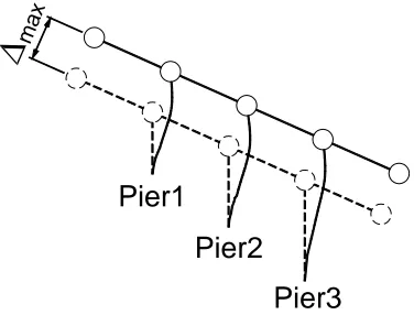
A second problem is applying a constant reduction factor for all structural systems of a certain class, as well as to all members in a structural system. Consider a bridge configuration with three piers at different heights as shown in Figure 2. For simplicity, the piers have the same yield (φy) and ultimate (φu) curvatures, and hence the same curvature ductility. Yield displacements are approximately proportional to the height square, as shown by Eq. 6 where h is the pier height.

3 /

2

h

y y =

φ

∆ Eq. 6

ma x

Pier1

Pier2

Pier3

Figure 2 Pier Ductility Demands

4. FUNDAMENTALS OF DIRECT DISPLACEMENT-BASED

DESIGN

The direct displacement-based design (DDBD) procedure utilizes the secant stiffness method and the equivalent damping approach to characterize the structure that is to be designed, as

an equivalent linear single-degree-of freedom (SDOF) structure. The DDBD approach aims at designing a structure to achieve a selected performance limit state under a selected earthquake intensity. The procedure must be combined with capacity design principles to ensure that plastic hinges form where intended, and to prevent any non-ductile modes of inelastic deformation from occurring.

In the case of multi-degree-of freedom (MDOF) structures, the DDBD characterizes such a structure by an equivalent SDOF oscillator with system mass (Msys) and system force

(Fsys) based on equal work done by both systems, see Figure 3a. This is based on the

substitute structure approach developed by Sozen and Shibata in 1976 [9]. The SDOF

hysteretic behavior is then described in terms of the secant stiffness at peak response (Keff)

After obtaining the equivalent damping, the design response spectrum is reduced through the use of a damping reduction factor. The displacements corresponding to, ξ,

damping (∆T, ξ%) can be related to the displacements for 5% damping (∆T, 5%) by the

EuroCode 8 [10] expression given in Eq. 7 for far field records and Eq. 8 for near

F₂ F₁

3

F

Fsys

sys

M

i

K

i

rK

eff

K F_m

y

F

sys

∆

∆

sys

∆

(a) SDOF Simulation (b) Equivalent Linearization Figure 3 Equivalent SDOF Structure Characterization

0% 5% 10% 15% 20% 25%

1.0 2.0 3.0 4.0 5.0 6.0

Displacement Ductility (µ)

Equiva

le

nt Dampin

g

Steel Member

R/C Beam

R/C Column

Unbonded Prestressing

Period (sec)

2.0 1.0

0.0 3.0 4.0 5.0 6.0

Di

sp

la

ce

me

nt

(m)

0.20

0.0 1.00

0.80

0.60

0.40

5%

15%

25% 35%

Teff

∆sys

µ

ξsys

(a) Equivalent Damping vs. Ductility (b) Design Displacement Spectra Figure 4 Obtaining Equivalent SDOF Structure Effective Period

field records. The damped spectra is then entered with the target displacement (∆m), which is selected in accordance with the desired performance limit state, to obtain the equivalent SDOF structure effective period (Teff), as shown in Figure 4b. The effective period is then

used to compute the effective stiffness (Keff) and the design base shear (VB) as given by Eq. 9

designed according to capacity design principles in order to guarantee the development of the desired failure mechanism.

5 . 0 % 5 , % , 2 7 ⎟⎟ ⎠ ⎞ ⎜⎜ ⎝ ⎛ + ∆ = ∆

ξ

T Eq. 7

25 . 0 % 5 , % , 2 7 ⎟⎟ ⎠ ⎞ ⎜⎜ ⎝ ⎛ + ∆ = ∆

ξ

T Eq. 8

2 2 4 eff sys eff T M

K =

π

m eff B

m V K

F = = ∆ Eq. 10

5. DESIGN LIMIT STATES

5.1 System Limit States

The SEAOC guidelines [5] define a structure performance level as the coupling between performance limit state and seismic demand (i.e earthquake intensities), while a performance objective is defined as a series of performance levels. Figure 5 shows typical seismic performance objectives for buildings, where SP refers to structural element performance

level and NP refers to nonstructural element performance level. For instance, the “Basic

Objective” line relates performance levels to earthquake intensities for normal buildings such as houses and offices; however, the “Enhanced Objective 1” line relates performance levels to earthquake intensities for more important structures such as schools, firehouses and hospitals.

(∆p). However, the near collapse limit state is expected when the structure utilizes 80% of its inelastic drift capacity. The guidelines also define 4 seismic hazard levels, 1 through EQ-IV with probability of exceedence dependent on local seismicity. For instance, in California the return periods for these earthquake intensities are, 25 years, 72 years, 2/3 of the MCE and the MCE, respectively. The MCE is the Maximum Considered Earthquake with a return period of 2,475 years.

Figure 5 Typical Seismic Performance Objectives for Buildings. Ref. [5] Table 1 Structural Performance Levels, Ref. [5]

Structural

Performance Level

Qualitative Description

System Displacement Limit

SP-1 Operational ∆y

SP-2 Occupiable ∆y + 0.3∆p

SP-3 Life Safe ∆y + 0.6∆p

SP-4 Near Collapse ∆y + 0.8∆p

SP-5 Collapse ∆y + ∆p

5.2 Drift Limits for a SDOF Structure

∆y ∆p

.3∆p .3∆p .2∆p .2∆p

Nominal Yield

SP-1 SP-2 SP-3 SP-4 SP-5

1 2 3 4 5

Displacement

Equivalent Seis

mic Force

= (Inelastic Displacement Capacity)

Structural Response Envelope

Figure 6 Illustration of Structural Performance Levels, Ref. [5].

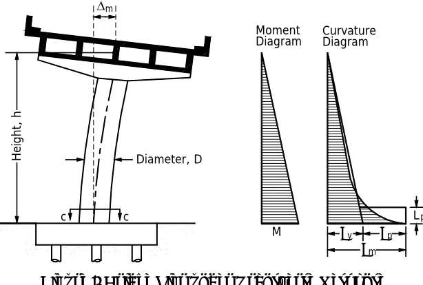
Consider the bridge pier under transverse response shown in Figure 7 where h is the

height of the pier, which extends from the face of the footing to the center of the superstructure, and D is the pier diameter. Also shown in the figure are the bending moment

and curvature diagrams at maximum response. The actual curvature distribution at yield will be nonlinear, however a linear approximation is adopted where φy is computed in terms of the

first yield φ’

y, maximum moment M and yield moment My as given by Eq. 11 where first

yield occurs when the reinforcement closest to the extreme tension fiber yield. As a result, the yield displacements may be estimated as in Eq. 12.

'

y y y

M M

_φ

φ

3

2

h

y y

φ

∆ Eq. 12

Height

, h

Diameter, D

c

c Lp

Moment Diagram

M

Diagram Curvature

φm

y

φ φp

m

Figure 7 Bridge Pier under Transverse Response

c

ε

d

c

s

ε φ

Figure 8 Pier Section and Limit State Strains (Section c-c)

c

mc

mc

ε

φ

) /(d c

ms

ms =

ε

φ

Once the design curvature has been established, based on strain criteria, the design displacement is calculated as given by Eq. 15. The length Lp is chosen such that the plastic

displacement (∆p) at the top of the cantilever, predicted by the simplified approach is the same as that derived from the actual curvature distribution [7].

h L h

p y m y

p y

m ₃ ( )

2

φ

φ

φ

− + =

∆ + ∆ =

The structural drift limit state is computed as ∆m/h, which should be compared with the code-specified drift limit for non-structural elements θd, and the lower from both values must be used in the design.

6. EQUIVALENT DAMPING APPROACH

6.1 Introduction

The equivalent linearization concept was first suggested by Jacobsen [11] in 1930. In his pioneering paper, Jacobsen attempted to obtain an approximate solution of the steady forced vibration with general types of damping. The original nonlinear system involves one damping term as given by Eq. 16 where m is the mass, k is the original system

stiffness and x is a harmonic displacement response.

n nx

c &

±

t F kx x c x

m&&± _n&n + = sinΩ Eq. 16

The previous nonlinear equation was replaced by an equivalent linear equation with the damping force replaced by a simpler and equivalent one of the form . The equivalent linear system equation of motion is given by Eq. 17. Note that both systems have the same mass and stiffness which results in equal initial periods for both systems.

x c₁&

t F kx x c x

m&&± 1&+ = sinΩ Eq. 17

The damping factor c1 was obtained assuming the response of both systems is

sinusoidal and of the from x = X.sin(Ω.t – ψ). By equating the work done by both systems

within a cycle of the response, the equivalent damping as given by Eq. 18 is obtained. Jacobsen carried out approximate solution of the forced vibration of a system with constant friction and velocity damping for four special cases on three different criteria of equivalent viscous damping force. The results were compared to experimental evidence and the three criteria gave approximately the same agreement with experiment. However, the one cycle criterion was superior at or near resonance.

dt t X

c

c _n n n 4 cosn .

2

1 1

1

1

∫

Ω + −

−_Ω Ω _Ω

≡

π

Note that the previous expression is only exact for the case where n = 1, since the response is harmonic, however it is approximate for any other case. Also if the equivalent system frequency equals the forcing function frequency, a harmonic response is expected and the sinusoidal assumption is still valid. Jacobsen’s attempt to approximate the nonlinear solution was proven to be successful by the many examples he solved and compared to the available exact or numerical solutions. The previous concept was adopted by many researchers to approximate the peak response of a yielding system as discussed in section 6.3. However, the mechanism by which the response of a yielding structure damps differs from the type of damping Jacobsen considered in the original approach. Furthermore, the excitation applied to the yielding system was not harmonic as Jacobsen assumed; instead, it was random earthquake type excitation. Part-II, section 3 includes a discussion of the added uncertainties to the approach that arise by applying it to earthquake excitations.

6.2 Equivalent Damping for a Yielding Structure

The equation of motion for a yielding structure is given by Eq. 19 where k(x) is a restoring

force that takes different forms. A typical example of a restoring force, known as the bilinear hysteresis, is shown in Figure 9. Note that ki is the initial stiffness, keff is the secant stiffness

at maximum response, xy is the yield displacement and xm is the maximum response. The

secant and initial stiffnesses are related from geometry by Eq. 20 where µ is the displacement ductility (xm/xy). The energy dissipated by this system through a cycle that passes through the

peak response (xm) equals the area bounded by the loop as given in Eq. 21 where WNL is the

energy dissipated by the nonlinear system. )

( ).

(x x F t k

x c x

m&&± &± = Eq. 19

µ

µ

=k r r

keff i Eq. 20

) 1 (

) 1 )( 1 (

4 2

+ −

− − =

r r

r x

k W_{NL eff m}

µ

µ

µ

Eq. 21

this system is given by Eq. 22 and the steady state response is given by Eq. 23 where Ω is the forcing function frequency and Φ is the phase angle. Since kinetic energy and potential energy (i.e strain energy) within one cycle of response equal 0, then the total energy dissipated by this system is equal to the work done by the damping force as given by Eq. 24 where WLS is the energy dissipated by the equivalent linear system.

Force

Ki

rKi

Keff

y

x xm

Fy

Figure 9 Yielding Structure - Bilinear Hysteretic Model

) sin(

1x kx F t

c x

m&&+ &+ = Ω Eq. 22

) sin(

)

(t =x Ωt−Φ

x m Eq. 23

[

]

= Ω

_∫

2

0

2

1

π

π

c x dt t

x c

W_{LS m m} Eq. 24

m

c

K

F(t) = F sin

Ω

Figure 10 Equivalent Linear System Representation

2

2 _{eq m}

LS k x

W =

ξ

In order to compute the equivalent damping, the energy dissipated by the original nonlinear and equivalent linear oscillators is equated. However, note that we have not specified the stiffness of the equivalent system (Eq. 25), hence, the equivalent damping will depend on our choice of that stiffness. Firstly, assume that the shift in the period is based on the secant stiffness, Keff, as given by Eq. 26 where Ti is the initial period, and then replace the

stiffness in Eq. 25 by Keff. Equate the energy dissipated by both systems to obtain the

equivalent damping relation given by Eq. 27. Secondly, select no shift in the period which means the equivalent system has the same stiffness of the nonlinear system Ki, which results

in a different equivalent damping relation as given by Eq. 28.

1

+ − =

r r T

T

i eff

µ

µ

Eq. 26

) 1

(

) 1 )( 1 ( 2 ) (

r r

r

eff

eq _{+ −}

− − =

µ

µ

µ

π

ξ

2

) 1 )( 1 ( 2 ) (

µ

µ

π

ξ

Figure 11 shows both damping values (based on secant and initial stiffnesses) plotted against displacement ductility for a bilinear factor of 10%. The figure also shows the period shift based on secant stiffness and apparently the period shift due to initial stiffness is one. Clearly, there is a significant difference between both damping values; secant stiffness proportional damping has a maximum of 33%, while initial stiffness proportional damping has a maximum of 14%.

0% 5% 10% 15% 20% 25% 30% 35%

1 2 3 4 5 6 7 8

Displacement Ductility (µ)

Eq

uival

en

t Damp

ing (ξeq)eff

(ξeq)i

(a) Secant and Initial Stiffnesses Proportional Equivalent Damping

1.00 1.20 1.40 1.60 1.80 2.00 2.20

1 2 3 4 5 6 7 8

Displacement Ductility (µ) Te

ff

/ T

i

(b) Secant Stiffness Proportional Period Shift (r = 10%)

Figure 11 (a) Secant and Initial Stiffnesses Proportional Damping (b) Secant Stiffness Proportional Period Shift

and non-structural elements. Thus, equivalent damping has two components: elastic and hysteretic. Elastic damping (ξv) is usually taken between 2%-5% for bridge columns. However, hysteretic damping is a function of the energy dissipated by the structural member due to ductile response as discussed earlier. Historically, these two values have been always added together to obtain the total equivalent viscous damping. However, a recent work by Priestley and Grant [12] indicated that viscous and hysteretic damping should not be added directly. In order to verify the design developed by DDBD, the assumptions for elastic damping made in the design and time history analysis need to be compatible. Therefore, if the designed SDOF structure is modeled in the time history analysis with elastic damping (ξTH) that is tangent stiffness proportional, then the elastic damping used in the design

(ξDDBD) should be modified using the following equations:

TH DDBD

λ

λ

ξ

ξ

Bilinear Model:

λ

λ

µ

λ

λ

µ

Therefore, if a structure is modeled in the analysis with tangent proportional elastic damping then only λ1 is needed to correct the design tangent proportional damping.

r r −

+ =

µ

µ

λ

1

1 Eq. 32

6.3 Literature Review

As mentioned earlier, the equivalent damping approach was first proposed by Jacobsen [11] in 1930. Jacobsen aimed at obtaining a simple solution for the steady-state response of a nonlinear system. The approach defines an equivalent linear system based on the following assumptions: (1) Sinusoidal response (2) Equivalent energy dissipated by both systems through one cycle at peak response and, (3) Both systems having the same initial period. Jacobsen’s approach works reasonably well for harmonic excitations, however, when applied to earthquake excitations the approach shows large errors. Subsequent to Jacobsen’s work, many researchers have adopted the concept and developed different definitions of equivalent systems, as reviewed by Jennings [13] in 1968.

In 1974, Gulkan and Sozen [14] introduced the definition of substitute damping. In their approach, the effective period corresponds to the secant stiffness at peak response. The substitute viscous damping was computed by equating the energy input into the system to the energy dissipated by an imaginary viscous damper over the period of excitation as given by Eq. 33 where

β

y&&

x& is the relative velocity of the SDOF frame. Using experimental results and Takeda’s hysteretic model [15], Eq. 34 was suggested to compute equivalent damping for reinforced concrete columns. Gulkan and Sozen compared the results of their approach with experimental results and with Jacobsen’s approach, and found them to be in good agreement.

∫

∫

⎠ ⎞ ⎜

⎜ ⎝

⎛ tf tf

s

s m x dt m yxdt

0 0

2

2

ω

⎟⎟ ⎠ ⎞ ⎜⎜ ⎝ ⎛ − + =

µ

ξ

ξ

Iwan and Gates [16], in 1979 applied a statistical approach to obtain the optimum effective period and equivalent damping. Six different hysteretic models and 12 earthquake records were considered in the study. The optimization process was based on minimizing the root mean square of errors between the displacement of a nonlinear system and an equivalent linear system. Iwan [17], 1980, proposed Eq. 35 and Eq. 36 to estimate period shift and equivalent damping ratio for a hysteretic model derived from a combination of elastic and Coulomb slip elements. Ti is the initial period.

939 . 0 ) 1 ( 121 . 0

1+ −

=

µ

i eff

T T

Eq. 35

371 . 0 ) 1 ( 0587 . 0 − + =

ξ

µ

ξ

Kowalsky [18], in 1994 utilized a shift in the period based on the secant stiffness at maximum response and Jacobsen’s approach to develop the equivalent damping relationship given by Eq. 37. Takeda’s hysteretic model [15] was considered (see Figure 3c) with an unloading factor of 0.5 and post yield stiffness equal to zero.

⎟⎟ ⎠ ⎞ ⎜⎜ ⎝ ⎛ − + =

µ

π

ξ

ξ

Recently Kwan et al. [19], in 2003 utilized the same approach suggested by Iwan to

propose empirical relations for equivalent damping and period shift. Six hysteretic models, 20 ground motions, and periods between 0.1 and 1.5 seconds were considered in the study. The proposed equations differ from previous empirical ones by accounting for the type of hysteretic model. Kwan et al. proposed Eq. 38 and Eq. 39 for elasto-plastic, moderately

degrading and slightly degrading hysteretic models (i.e ductile steel and reinforced concrete structures).

µ

µ

µ

π

µξ

ξ

More recently, Miranda and Lin [20], in 2004 proposed a new shift in the period and equivalent damping relationship based on 72 earthquake time histories. The relationships were obtained by minimizing the error for each period as opposed to Iwan’s approach [17] of averaging the error over all periods. Miranda and Lin expressed the new relationships in terms of strength ratio R as given by Eq. 40 instead of displacement ductility as usual. In Eq.

40 m is the system mass, Sa ordinate of spectral acceleration and Fy is the system yield

strength. Period shift and equivalent damping are given by Eq. 41 and Eq. 42, respectively. The new proposed relationships showed significant improvement in predicting nonlinear system peak response in the short period range of the spectra.

y a

F S m

R = Eq. 40

) 01 . 0 027 . 0 )( 1 (

1 1.8 _1.6

i i

eff

T R

T T

+ −

+

= Eq. 41

) 002 . 0 02 . 0 )( 1

( _2.4

i v

eq

T R− +

+

=

ξ

ξ

7. RESEARCH OBJECTIVES

As mentioned earlier, the primary objective of this dissertation is to contribute to the advancement of DDBD in general and in particular to multi-span bridge structures. The objectives of this work are summarized as follow:

8. REFERENCES

2. This research aimed at suggesting new equivalent damping relationships so that any structure designed with DDBD will better meet its desired performance objective.

3. This research also aimed at developing a simplified approach to select target displacement profiles for multi-span bridges. The approach should eliminate the need for the iterative procedure in selecting target profiles.

4. Finally, this research aimed at evaluating the DDBD for multi-span bridge structure in order to obtain a preliminary quantification of the procedure accuracy for MDOF bridge systems.

1. Priestley M.J.N., Seible F. and Calvi G.M. Seismic design and retrofit of bridges. John Wiley and Sons, Inc 1996; New York, NY.

2. Uniform Building Code (UBC), Volume 2, Structural Engineering Design Provisions,

International Conference of Building Officials; 1997.

3. International Building Code, IBC 2000 – Section 1615: Earthquake Loads, Site Ground

Motion. International Code Council Inc 2000; Falls Church, VA.

4. AASHTO LRFD Bridge design specifications, second edition, American Association of

State Highway and Transportation Officials 1998; Washington, D.C.

5. Structural Engineers Association of California – Vision 2000. Conceptual Framework for Performance Based Seismic Engineering of Buildings, SEAOC 1995; Sacramento,

CA.

6. Priestley MJN., Calvi G.M. and Kowalsky M.J. Direct Displacement-Based Seismic Design of Structures. IUSS Press 2005; Pavia, In Preperation.

7. Paulay T. and Priestley M.J.N. Seismic design of reinforced concrete and masonry buildings. John Wiley and Sons, Inc. 1990.

8. Priestley, M.J.N. Myths and fallacies in earthquake engineering – conflicts between design and reality. Bulletin, NZ National Society for Earthquake Engineering 1993;

26(3): 329-341.

9. Shibata A. and Sozen M. Substitute structure method for seismic design in R/C.

10. EuroCode 8. Structure is seismic regions – Design. Part 1, General and Building. May 1988 Edition, Report EUR 8849 EN, Commission of European Communities.

11. Jacobsen L.S. Steady forced vibrations as influenced by damping. ASME Transactione

1930; 52(1): 169-181.

12. Priestley M.J.N. and Grant D.N. Viscous damping in seismic design and analysis.

Journal of Earthquake Engineering, 2004; to appear.

13. Jennings P.C. Equivalent viscous damping for yielding structures. Journal of Engineering Mechanics Division, ASCE 1968; 90(2): 103-116.

14. Gulkan P. and Sozen M. Inelastic response of reinforced concrete structures to earthquake motion. ACI Journal 1974; 71: 604-610.

15. Takeda T., Sozen M. and Nielsen N. Reinforced concrete response to simulated earthquakes. Journal of the Structural Division, ASCE 1970; 96(12): 2557-2573

16. Iwan W.D. and Gates N.C. Estimating earthquake response of simple hysteretic structures. Journal of Engineering Mechanics Division,ASCE 1979; 105: 391-405.

17. Iwan W.D. Estimating inelastic spectra from elastic spectra. Earthquake Engineering and Structural Dynamics 1980; 8: 375-388.

18. Kowalsky M.J. Displacement-based design-a methodology for seismic design applied to RC bridge columns. Master’s Thesis 1994; University of California at San Diego, La

Jolla, California.

19. Kwan W.P. and Billington S.L. Influence of hysteretic behavior on equivalent period and damping of structural systems. Journal of Structural Engineering, ASCE 2003;

129(5): 576-585.

20. Miranda E.and Lin Y. Non-iterative equivalent linear method for displacement-based design. 13th World Conference of Earthquake Engineering, 13WCEE 2004; Vancouver,

PART-II

EQUIVALENT DAMPING IN SUPPORT OF DIRECT

DISPLACEMENT-BASED DESIGN

Hazim M. Dwairi, Mervyn J. Kowalsky and James M. Nau

Based upon a paper submitted to:

EQUIVALENT DAMPING IN SUPPORT OF DIRECT

DISPLACEMENT-BASED DESIGN

Hazim M. Dwairi, Mervyn J. Kowalsky and James M. Nau

Department of Civil, Construction and Environmental Engineering, North Carolina State University, Campus-Box 7908, Raleigh, NC-27695, USA

SUMMARY

The concept of equivalent linearization of nonlinear system response as applied to direct displacement-based design is evaluated. Jacobsen’s equivalent damping approach combined with the secant stiffness method has been adopted for the linearization process. Four types of hysteretic models and a catalog of 100 earthquake records were considered. The evaluation process revealed significant errors in approximating maximum inelastic displacements due to overestimation of the equivalent damping values in the intermediate to long period range. Conversely, underestimation of the equivalent damping led to overestimation of displacements in the short period range, in particular for Teff < 0.4 seconds. The scatter in the

results ranged between 20% and 40% as a function of ductility, primarily due to earthquake characteristics. New equivalent damping relations for 4 structural systems, based upon nonlinear system ductility and maximum displacement, are proposed. The accuracy of the new equivalent damping relations is assessed, yielding a significant reduction of the error in predicting inelastic displacements. Minimal improvement in the scatter of the results was achieved, however.

KEY WORDS

1. INTRODUCTION

Approximate solutions for nonlinear response of yielding structures have gained a wide interest as a simple analysis technique for seismic design procedures, such as Direct Displacement-Based Design (DDBD). One of the techniques used involves replacing the nonlinear structure with an equivalent linear structure whose maximum displacement response will be approximately equal to the original nonlinear structural response. The equivalent structure approach was first suggested by Jacobsen in 1930 [1]. At the time, Jacobsen suggested an approximate solution of the steady-state response of a nonlinear oscillator by defining an equivalent linear oscillator. In Jacobsen’s approach, both oscillators have the same natural frequency and dissipate equal energy per cycle of sinusoidal response. In 1993 [2], the equivalent structure concept was adopted for Direct Displacement-Based Design (DDBD) as a simple means of designing a yielding structure for a predefined performance level.

Among a number of methods used for nonlinear response approximation, Jacobsen’s equivalent linearization approach was adopted for Direct Displacement-Based Design DDBD because of: (1) its simplicity, (2) the ease with which the relations between hysteretic shape and equivalent damping are obtained, and (3) the familiarity with elastic spectra for design. Alternative methods, such as inelastic spectra, do not provide sufficient benefit to warrant the added complexity, although they certainly could be adopted for DDBD [3].

Jacobson’s [1] approach to compute the equivalent damping. Miranda concluded both methods yielded reasonably good estimates of maximum displacement in the long period range, while both approaches overestimate displacements in the short period range. Iwan [8] selected a shift in the period and equivalent damping based on minimizing the error between exact and approximate displacements. Miranda [5] concluded that Iwan’s method yielded better results in the long period range than the previous two; however, displacements were underestimated in the short period range. It is important to point out that empirical equations, which have variable period shift, are not directly related to the design base shear. Furthermore, these equations usually do not take the hysteretic model shape into consideration, which makes them less attached to structural behavior and consequently less appealing for design procedures.

Recently, Ramirez et al. [9] validated the simplified methods of inelastic analysis

suggested by the 2000 NEHRP provisions. The NEHRP provisions suggest an equation

similar to Eq. 4 in order to estimate the equivalent damping for a bilinear hysteretic model like the one shown in Figure 1. The NEHRP equivalent damping is based on Jacobsen’s

approach and the secant stiffness method. It will be shown later that the damping values given by Jacobsen’s approach are overestimated and need to be reduced. More recently, Kwan et al. [10] proposed empirical relations for equivalent damping and period shift

derived from minimizing the root mean square of errors between the displacements of nonlinear systems and equivalent linear system. Six hysteretic models, 20 ground motions, and periods between 0.1 and 1.5 seconds were considered. The proposed equations differ from previous empirical ones by accounting for the type of hysteretic model. However, they yielded close estimates to the equivalent damping given by Iwan’s [8] and Galkan and Sozen’s [6] methods for reinforced concrete members.

2.

3.

PAPER LAYOUT

In this paper, Jacobsen’s [1] equivalent damping approach combined with the secant stiffness method is evaluated for 4 hysteretic systems, various ductility values, and 100 real earthquake records. A review of Jacobsen’s approach is provided with a brief discussion of the assumptions made. The assessment algorithm used to evaluate the equivalent damping approach is then discussed. Modified equivalent damping relations are obtained based on a best fit of the results from 100 earthquakes for the 4 hysteretic systems.

JACOBSEN’S EQUIVALENT DAMPING APPROACH

As mentioned earlier, the equivalent damping approach was first proposed by Jacobsen [1] in 1930. Equivalent linear systems with fictitious equivalent damping were proposed to approximate the steady-state response of a damped nonlinear system. The basic assumptions in the approach are:

1. Both systems have the same initial period (i.e. no period shift),

2. Both systems undergo harmonic steady-state response given by a constant amplitude sinusoidal function of the form Xsin(ωt - ψ),

3. Both systems are at resonance, and

4. The energy dissipated per cycle of the assumed motion by the nonlinear system equals the energy dissipated per cycle by the equivalent system.

equivalent damping approach. Considering the average value of the energy dissipated through all cycles is expected to yield lower equivalent damping values.

The equivalent damping along with the secant stiffness yields the same period shift (Teff/Ti) for all hysteretic models. As a result, the equivalent damping values obtained by this

approach are usually higher than those obtained by other techniques which consider less period shift. Thus, applying the equivalent damping approach for the theoretical case of a rigid-perfectly-plastic loop, which dissipates more energy than any other model, results in a maximum equivalent damping of 2/π.

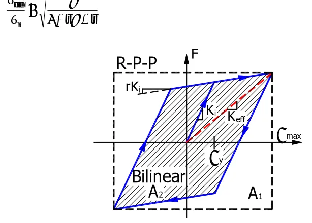
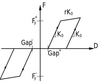
Jacobsen’s equivalent damping combined with the secant stiffness at maximum response is applied for a bilinear hysteretic model shown in Figure 1. The Bilinear model considered has initial stiffness Ki, secondary stiffness rKi, yield displacement ∆y and

maximum displacement ∆max. It can be shown that the equivalent system has a period shift given by Eq. 1 where Ti is the initial fundamental period of the structure and µ is the

displacement ductility (∆max/∆y).

r r T

T

i eff

− + =

µ

µ

1 Eq. 1

F

Ki

rKi

max

Keff

A

∆

∆

2

A

Bilinear

R-P-P

Figure 1 Equivalent Damping for Bilinear and R-P-P Hysteretic Models

damping is proportional to the energy dissipated by the hysteretic model, the equivalent damping for any shape is given by Eq. 2 and Eq. 3 where ξv is the initial elastic damping in the nonlinear system, ξhyst is the hysteretic damping due to the energy dissipated, A1 is the

area of the hysteretic loop and A2 is the area of the R-P-P loop which passes through

maximum displacement. In Eq. 2, viscous and hysteretic damping are added; however, the work by Grant et al. [11] has indicated that viscous and hysteretic damping should not be

added directly. If the structure exhibits viscous damping which is proportional to tangent stiffness, this damping value should be reduced prior to adding it to the hysteretic component. Based on time history analyses, Grant et al. [11] identified this factor to be

dependent upon the level of ductility. However, if the viscous damping term is small (about 2% or less), the effect of the correction factor is minimal. In this paper, viscous damping and hysteretic damping have been added directly as given by Eq. 2.

hyst v eq

ξ

ξ

ξ

2 1

2

A A

hyst

π

ξ

Substituting in the previous equations for the bilinear loop shown in Figure 1, yields the equivalent damping relation given by Eq. 4. Application of Jacobsen’s approach to other hysteretic models will be discussed in section 5.

( )

(

₍

)(

)

₎

r r

r

v Bilinear eq

− +

− − +

=

µ

µ

µ

π

ξ

ξ

1 1 1 2

Eq. 4

4. REVIEW OF DIRECT DISPLACEMENT-BASED DESIGN

equivalent elastic system properties and elastic response spectra reduced for equivalent damping values. The basic steps of the design procedure for SDOF structures are:

1. Obtain target-displacement (∆t): Based on strain or drift criteria which define the

desired level of performance.

2. Estimate equivalent viscous damping (ξeff): Utilizing the target-displacement and

estimated yield displacement, equivalent damping values are obtained as discussed in the previous section.

3. Determine equivalent structure period (T ): eff Utilizing the target-displacement and

elastic spectra reduced for the equivalent damping value from step 2, an effective period is determined as shown in Figure 2.

4. Evaluate effective stiffness (K ) and design base shear (V ):eff B Utilizing the

effective period, the target displacement (∆t) and the structure mass (m), effective stiffness and design based shear are easily calculated as given in Eq. 5 and Eq. 6, respectively.

2 2

4 eff eff

T m

K =

π

t eff

B K

V = ∆ Eq. 6

The steps of the DDDB approach can be combined into a base shear equation given by Eq. 7. In this equation, the 5% damped elastic spectrum is reduced according to the equivalent damping ratio in accordance with EuroCode 8 [12]. Also, Eq. 7

assumes a linear displacement spectrum defined by a corner period, Tc, and corner

displacement, ∆c, as shown in Figure 2.

eq c

c

t B

T m V

ξ

π

+ ⎟⎟ ⎠ ⎞ ⎜⎜ ⎝ ⎛ ∆ ∆ =

2 7

4 2 2

Eq. 7

is achieved. For more information on the Direct Displacement-Based Design approach, refer to [13].

%5

%10

%15

%20

0 1 2 3 4

0.00 0.25 0.50 0.75 1.00

Spectral D

isplacement (m)

Period (sec)

5

Target Displacement

Equivalent Damping

Ef

fe

ctive Pe

riod

Tc= ∆c

Teff ∆t=

=

ξeq ( )

Figure 2 Determination of Equivalent SDOF Properties

5. EVALUATION PROCEDURE AND RESUTS

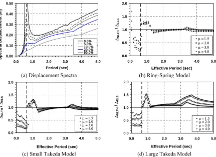
In order to evaluate the displacement-prediction capability of equivalent linear structures (ELS) defined by Jacobsen’s equivalent damping and the secant stiffness method, a large number of nonlinear time history analyses (NLTH) were conducted, the parameters of which will be described later. In each case, the displacement of the nonlinear oscillator was obtained using inelastic time-history analysis (NLTH) and compared with the displacement of the equivalent linear structure (ELS). Since equivalent damping values vary with the hysteretic model considered, four models were selected for this study as shown in Figure 3. The selected parameters which define the size of the loops, and hence the equivalent damping are given in Table 1. The small Takeda model resembles a reinforced concrete column, while the large Takeda represents a reinforced concrete beam. The Elasto-Plastic model represents a steel member, while the Ring-Spring resembles a post tensioned column or wall, as well as a seismic isolation device.

Table 1 Parameters Considered for Hysteretic Models

Parameter Ring-Spring Large Takeda Small Takeda

r 0.1 0.0 0.0

α N.A. 0.0 0.5

β N.A. 0.6 0.0

rl 0.04 N.A. N.A.

rs 1.0 N.A. N.A.

period shifts have been plotted in Figure 4. Since the assumed bilinear factors for Takeda’s model and the Elasto-Plastic model are equal to 0.0, the period shifts for both models are equal according to Eq. 1. The Ring-Spring model has less period shift since it has a bilinear factor of 10%.

Ring-Spring Hysteretic Model (r = 0.1, rl = 0.04, rs = 1.0):

(

)

µ

µ

µ

µ

π

ξ

Takeda’s Hysteretic Model [15]:

⎟⎟ ⎟ ⎟ ⎟ ⎟ ⎠ ⎞ ⎜⎜ ⎜ ⎜ ⎜ ⎜ ⎝ ⎛ ⎥ ⎥ ⎦ ⎤ ⎢ ⎢ ⎣ ⎡ ⎟⎟ ⎠ ⎞ ⎜⎜ ⎝ ⎛ ₋ − ⎥ ⎦ ⎤ ⎢ ⎣ ⎡ − ⎟⎟ ⎠ ⎞ ⎜⎜ ⎝ ⎛ ₋ − ⎥ ⎦ ⎤ ⎢ ⎣ ⎡ + ⎟⎟ ⎠ ⎞ ⎜⎜ ⎝ ⎛ ₋ − − ⎟ ⎠ ⎞ ⎜ ⎝ ⎛ = − − 2 2 1 1 1 1 4 1 1 1 2 1 1 1 4 1 4 3 1 2

µ

γ

µ

β

γ

µ

µ

β

µ

γ

βµ

γ

µ

π

ξ

hyst Eq. 9

1

+ −

=rµ r

γ Eq. 10

Elasto-Plastic Hysteretic Model:

(

)

µ

µ

π

ξ