Extending the Kingman General Arrival, General Service Queuing Approximation to Overhead Allocation and Service Pricing.

(1)

ASHBAUGH, BRADLEY KENNETH. Extending the Kingman General Arrival, General Service Queuing Approximation to Overhead Allocation and Service Pricing. (Under the direction of Michael G. Kay and Robert B. Handfield).

In addition to recording transactions, accounting systems are used to evaluate performance, help determine what to produce, allocate overhead, and determine break-even pricing. Most accounting systems are well suited to calculate average costs but are less successful in determining marginal costs and most ignore arrival and process variability effects. Only time-driven activity-based costing attempts to measure process variability, and no established system measures the costs of arrival variability. From queuing theory, it is known that variability affects work-in-process inventory (WIP) for products and average wait times for services. Higher variability causes higher WIP and higher average wait times for a given resource utilization level. This results in higher inventory costs for products and lower customer satisfaction for customers.

This dissertation continues the work of using allocated clearing functions to account for variability in production. Using a two product, three resource production facility, clearing functions are used to charge for WIP as resources become congested. This system is

(2)

cost differentials. Second, an MRI facility with both scheduled patients and emergency room patients is modeled to determine how much more capacity is needed for emergency room patients to maintain a required level of service versus scheduled patients. Per patient capacity needs are then used to justify differential pricing between the different patient types.

(3)

(4)

by

Bradley Kenneth Ashbaugh

A dissertation submitted to the Graduate Faculty of North Carolina State University

in partial fulfillment of the requirements for the degree of

Doctor of Philosophy

Industrial Engineering

Raleigh, North Carolina 2019

APPROVED BY:

________________________________ ________________________________

Robert Handfield Michael Kay

Co-chair of Advisory Committee Co-chair of Advisory Committee

________________________________ ________________________________

(5)

DEDICATION

This dissertation is dedicated to

My wife who worked very hard to help me reach my dream My son who pushed me to finish

My mother and father who helped me love school My friends who encouraged me

(6)

BIOGRAPHY

Bradley Ashbaugh was born in Los Angeles, California as the son of a Drama / English / History high school teaching and World War II veteran father and a Math / Computer high school and later community college teaching mother. At age 3 he moved to San Clemente, California where he grew up loving competitive swimming, water polo, and surf riding. The love of the water and the beach paid off as he became a lifeguard at San Clemente, Doheny, and San Onofre State Beaches. In addition to saving hundreds of lives, the job was important as it enabled him to pay his way through college.

He went to San Diego State University starting in Aerospace Engineering. He later switched to Mechanical Engineering when he saw deep budget cuts in the aerospace industry with the fall of the Soviet Union. While at SDSU, he was fortunate to become involved in student government where he had the opportunity to serve as President of the Associated Engineering Student Council leading and participating in College of Engineering wide events. He was honored to be inducted into Tau Beta Pi, Pi Tau Sigma, and the Order of Omega honor societies as well as receive a university award for Outstanding Contribution to Student Government. He also went on to receive a minor in Economics and was an intern for the City of San Diego Traffic Engineering Department. Despite successfully graduating, something was amiss. He loved engineering and economics but lacked intuition and passion for machine design. He had a talent for Operations Management and Computer

Programming, so he decided to enter graduate school in a major that combined Engineering, Operations, and Economics.

(7)

He enjoyed his classes and was incredibly lucky to be assigned as teaching assistant to IE 498: Senior Design. Working with Dr. William Smith and Dr. Wilbur Meier to help student teams solve real industry problems was his dream assignment. He found that he had an ability to quickly see through problems at industry facilities which helped earn him the Outstanding Teaching Assistant award from Industrial Engineering. He was also fortunate to meet his future wife, Maria, a Furniture Manufacturing and Management degree recipient from NC State University and jointly an Interior Design degree holder from Meredith College.

(8)

(9)

ACKNOWLEDGMENTS

I have been fortunate to learn from amazing professors. My journey in Industrial Engineering started with Mr. Clarence Smith and Dr. Steve Roberts offering me a teaching assistantship so I could afford Graduate School. I took classes from Dr. Richard Bernhard and Dr. William Smith my first semester and they became my earliest mentors. I am a better businessperson from my experience with Dr. Smith and I am a better academic from Dr. Bernhard. I was fortunate to also witness the teaching styles of Dr. Thom Hodgson, Dr. Russell King, the late Dr. Wilbur Meier, and Dr. James Wilson. My Accounting instructor, Dr. Gilroy Zuckerman was the first to tell me that I had a talent for teaching on the university level. This education served me well in my consulting and business career.

Upon returning to NC State University for my PhD, I was lucky to get to learn from Dr. Paul Cohen, Dr. Yahya Fathi, Dr. Ola Harrysson, Dr. Julie Ivy, Dr. Dave Kaber, Dr. Michael Kay, Dr. Yuan-Shin Lee, Dr. Reha Uzsoy, Dr. Richard Wysk, and Dr. Robert Young in addition to Drs. Bernhard, Hodgson, King, and Wilson. Although the subject matter varied among courses, I try to bring lessons I have learned from them to be a better instructor.

I also want to thank Dr. David Baumer from the Poole College of Management for giving me the opportunity to teach Operations Management at NC State and the other

(10)

(11)

LIST OF TABLES

Table 3-1: Numerical Example Common Coefficients ... 21

Table 3-2: Clearing Function Segments ... 21

Table 3-3: Model Output from CF Formulation ... 24

Table 3-4: Duels of the Optimal Product Mix for Both the LP and CF Formulation ... 25

Table 3-5: Contribution Margin of the Optimal Product Mix for Both LP and CF Model .... 36

Table 3-6: Optimal Values Between CF Models ... 41

Table 3-7: Comparison of CF Formulation Duels ... 41

Table 3-8: Comparison of Duels Between LP and CF Formulations with Product Interdependencies ... 44

Table 4-1: Comparison of 3 Segment versus 20 Segment Clearing Function ... 55

Table 4-2: Machine 1 Enhanced Excel Clearing Function ... 55

Table 5-1: LP Output for Symmetric Parallel Machines ... 62

Table 7-1: Overhead Allocation Summary by Method and Patient Type ... 71

(14)

LIST OF FIGURES

Figure 1-1: WIP vs Utilization ... 5

Figure 3-1: Graph of Clearing Function Segments ... 22

Figure 4-1: 20 Segment Clearing Function ... 52

Figure 4-2: Chapter 3 Model Replaced with 20 Segment Clearing Function... 54

Figure 4-3: 20 Segment Clearing Function with High Variability in Machine 2 ... 58

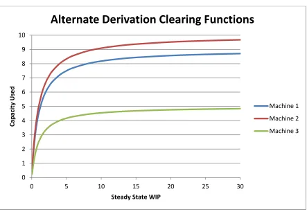
Figure 5-1: Graph of Clearing Functions with 1 through 5 Identical, Parallel Machines ... 61

Figure 7-1: MRI Time Estimates from Advanced Imaging in Missoula, MT ... 68

(15)

CHAPTER 1:

Introduction

What is the cost of variability? This is a simple question that does not often have an easy answer. We know from the Law of Variability (Hopp and Spearman 2001) that the more variability to a process, the less efficient the process. Variability can be observed in many forms. There can be variability in worker productivity, machine performance, quality, product variety, incoming materials, tooling, environmental factors, employee absenteeism, learning curves, training, education, physical ability, morale, machine dependability, and other factors. There is variability of customer arrivals, expectations, degree of customization, tastes, and in the medical profession, drug efficacy, anatomical variations, ability to fight infections, and attitude. This dissertation provides a methodology that answers the question: how do we account for this variability when it comes to pricing or overhead allocation?

(16)

trying to quickly purchase a few items are likely to look elsewhere to buy their products. The same phenomena can be observed in factories when larger orders reach the factory floor, when batches of parts arrive at a machine, a factory recovering after a machine breakdown, and even in the loading and unloading of trucks. In each case, this variability can

immediately mean either paying employees for no work, losing potential sales due to short-term long lines, or having to pay employees overtime should the backups occur at the end of shift. Secondary effects include needing longer lead times to fill orders which can decreases customer service, increase inventory, or require more surge capacity. Additionally, increasing lead time reduces forecasting accuracy as forecasts are less accurate farther in the future.

Production planning, product costing, and overhead allocation are all important functions of both manufacturing and service organizations. Profitable enterprises are set pricing or reduce costs such that both fixed and variable overhead can be fully absorbed in the products or services rendered. However, competitive pressures often tempt management to limit capacity in order to reduce overhead but at a cost of increased WIP, customer waiting, or system cycle time. In addition, when there is arrival or process variability, manufacturing and service systems operate less efficiently. Because many organizations measure product or service profitability through their accounting systems, it is important to choose a system with an overhead allocation schema that is aligned with the optimal product mix problem. If the system was also sensitive to the effects of variability, managers would have a powerful tool to direct process improvement resources to opportunities that have greater positive impact on operational performance and profitability.

(17)

There have been several attempts that work well depending on the number of products, the number of resources used, and the number of resource constraints. A core problem with accounting systems is that they are usually designed to assign costs and profits once

production and sales have already occurred. They are less reliable as a means of planning and pricing. Provided is a quick summary of some strengths and weaknesses of several

managerial accounting allocation schemes.

1. Full absorption costing is the most traditional accounting system and has been used for over a century. It is not without flaws or detractors. Overhead is applied to products via a primary overhead driver. In many applications this driver is direct labor. A weakness of this approach is that it often drives attention to reducing the driver inputs to a product or facility in order to reduce the overhead assigned. The factory may have the exact same total labor charges but be able to shift large overhead charges to other products or facilities by reducing the quantity of labor considered direct, should direct labor be the overhead driver. Relatively, this kind of accounting system provides little incentive to reduce overhead versus the incentive to shift overhead to others.

2. Direct costing, or marginal cost accounting, does not assign fixed overhead to products and services. If one were to look at fixed overhead costs as strictly sunk costs, this makes some sense. However, this makes capital budgeting difficult as investment may not be recaptured with direct costing and has been blamed for the failure of several large companies including Braniff Airways.

(18)

planning. The additional detail makes the system more complex and has another drawback of not always being aligned with or recommending the optimal product mix, especially when average costs and marginal costs diverge.

4. Throughput accounting works very well at recommending the most profitable production plan when there is a single constrained resource capping production. Although throughput accounting can be very useful, it is not generally accepted accounting for use in financial accounting or to determine transfer pricing.

5. Linear programming allocation systems will allocate overhead while preserving the optimal product mix no matter how many constrained resources are in a facility. However, traditional linear programming allocation systems require that resources be utilized 100% in order for them to have shadow prices and the ability to assign

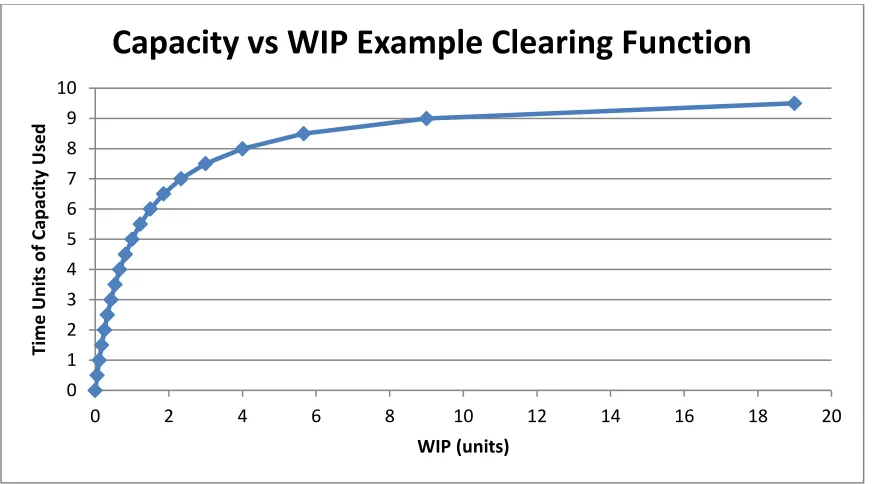
overhead to them. It is a well-known result from Queuing Theory that is very difficult to achieve 100% utilization, especially when there is any arrival variability or process variability. The more variability at a resource, the larger the work-in-process

(19)

Figure 1-1: WIP vs Utilization

6. Finally, time-driven activity-based costing captures some of the process variability by charging for various sources of different process times and creating time equations based on which factors are present. This richer breakdown of processing time is certainly useful. However, arrival variability is ignored. The M/D/1 queuing model, despite having fully deterministic (and constant) service times, still shows the effect of just arrival variability, albeit at half of the rate of the traditional M/M/1 queue.

Because these traditional and alternative accounting systems fail to fully account for both arrival and process variability, they are likely to overestimate resource and system output. One common way to prevent this is for planning to cap available capacity at 80% of theoretical capacity for service systems and 85% of theoretical capacity for manufacturing resources. There are at least three potential problems with this approach. One is that the

0.5 0.6 0.7 0.8 0.9 1

WIP

Utilization

WIP M/M/1

(20)

threshold may be wrong for a particular process or resource. If variability is low, output will be arbitrarily constrained. Conversely, if variability is high, the adverse effects of high WIP and cycle time will add costs and complexity to the system while still missing output goals. A second potential problem is a missed opportunity to focus resources on eliminating process variability and for scheduling to help reduce arrival variability. If the accounting is content with output based on 80 – 85% utilization, why strive for better? A third potential problem is a wasted opportunity to price products, services, or customers better. Products or services with more variability cost the company more and should not be subsidized by lower variability offerings unless there is a compelling business case. Also, consider a company with two different major customers. A customer that brings in steady business costs the company less than a customer with infrequent but urgent requests. A better understanding of how each customer affects costs can lead to better pricing or even turning away unprofitable customers.

(21)

level of capacity utilization the system is likely to support economically. In addition, the model will calculate shadow prices for resources employed and many will be nonzero even when utilization is less than 100%. This will allow managers to better determine pricing, capital budgeting for new capacity, and a way to estimate the potential to increase profits through variability reduction initiatives. In addition, it may be possible to observe practical bottlenecks from resources with higher theoretical capacity but higher variability than other resources. A third model will use clearing functions derived from G/G/m queuing where single machines can be replaced with multiple identical parallel machines.

A business case for the first half of this dissertation follows. Imagine a simple production shop where there are three machines. One machine is shared between two products while the other two machines are dedicated to each product. The shared machine could be a drilling machine with little to no setup between products. The dedicated machines may be shapers that are calibrated to the specific shapes of the two products. The products have different machine needs and sell for different prices. However, it is desired that the overhead for this machine shop be fully assigned to its products. Chapter 3 shows how this allocation should take place, when accounting for different arrival variability and process variability is resource dependent, not product dependent. Chapter 4 will provide the derivation and implementation of an alternative clearing function formulation. Finally, the model will be extended to multiple parallel machines in Chapter 5.

(22)

departments, or in this hypothetical case, patients. The model will have a resource shared between two products, customers, or departments each with different arrival and process variability. A two-step optimization problem using clearing functions to determine how much of the resource capacity, both used and unused, should be applied to each product, customer, or department. Multiple parallel resources serving both customers will also be tested versus dedicated resources to see if and where dedicated resources might produce superior results. A compelling business case for is easy to construct. Imagine a hospital with its many high value resources such as operating rooms, diagnostic equipment, and specialized

physicians. How should it price its services? Certainly, services should be priced to at least cover their direct costs. To be fully profitable, they need to price to also cover their fixed overhead costs. If the pricing is not competitive for any service, specialty groups can form and siphon off patients forcing other hospital services to charge more potentially making additional services uncompetitive. One way to try to stay competitive is to make sure these high value resources are all highly utilized. However, we know from queuing that highly utilized resources generate long waits and crowded waiting rooms. We also know that the more variability involved in either arrival or processing time increases line length and wait times.

(23)

time. Both scheduled patients and ER patients inherently require some process variability. According to Advanced Imaging, MRI scan times range from 20 minutes to one hour depending on the body part to be scanned. Patients may be slow to load, there may be stops to clean up from messy patients, tracer dye might be slow to reach the desired imaging sites, and patients can inadvertently move requiring rescans. In a hospital setting, patients with long wait times can result in decreased customer satisfaction at best and at worst

cancellations, loss of future business, diminished patient outcomes, and even patient death. Therefore, despite the large capital costs associated with high technology diagnostic equipment, it may be prudent to have some planned unused capacity built into a schedule. Two questions arise: how much extra capacity do we need and how do we allocate the costs of this extra capacity to the patients?

One method is to apply direct costs to all patients using the equipment and share the extra capacity costs evenly across all patients based on averages. For example, if the MRI averages 20 patients over a 24-hour period, charge each patient 20/24 or 5/6 of an hour for the MRI’s overhead costs. However, we know that we need more additional capacity to serve ER patients than those regularly scheduled due to the higher arrival and process variability these patients have. Charging all patients the same for the overhead of the MRI can have an adverse effect on the hospital when there are specialty MRI facilities that do not need to be available for emergency patients. The specialty MRI facility can schedule to reduce

(24)

Another option is to charge scheduled patients overhead based on just the time they use the machine. All the overhead from the extra capacity can be applied to the ER patients. In practice we would see MRI bills from scheduled appointments much lower than the same MRI from ER patients. Let us return to the example where the MRI averages 20 patients in a 24-hour period. Let us further stipulate that there are 5 ER patients, on average, each day. The 15 scheduled patients would just be charged their time on the machine. Each ER patient would be charged their time plus 1/5 of the total unused average time left in the day. If each MRI averaged 1 hour, each emergency room patent will be charged for 1.8 hours. Now imagine that total time on the MRI machine averaged 30 minutes per patient. Now the ER patients will be paying for the 30 minutes plus 14/5 hours of the unused capacity, a total 3.3 hours or 198 minutes. This would help the hospital price scheduled MRI’s competitive with specialty MRI centers. However, the competition can cry foul and with good reason. The hospital is now subsidizing its scheduled MRI service with ER patients.

Chapter 6 of the dissertation proposes a third way to allocate the capacity. Using the steady state queuing results derived from the Kingman VUT approximation for G/G/1 queuing, we can determine how much capacity should be scheduled for non-urgent patients and how to allocate unused capacity between patients for pricing purposes. This MRI example has some features different from steady state queuing. Steady state queuing uses first-in first-out (FIFO) scheduling. A hospital will certainly prioritize the MRI machine to critical ER patients. However, the model should give insight and help develop intuition in scheduling and pricing high value resources, including MRI machines and operating rooms.

(25)

another customer. Extra capacity will need to be set aside for the second customer and there needs to be a fair and rational way to assign capacity costs. The analysis will also be

beneficial to a company that has two versions of the same product. The first version might have a steady production stream while the second might be an older model that the firm refuses to terminate support for. The model should provide better estimates of the true cost of the second, older version and see if it should be retired if its marginal costs exceed the

marginal revenue of the line. Returning to health care, the model could provide capacity and costing guidance for a physician or nurse with responsibilities for two or more departments within a hospital.

Finally, simulation will be used to make sure that models yield appropriate results. Using steady-state queuing is useful to help make the math less complicated. However, it is important to note that startup effects will make the results less accurate when period length is too short. Simulation will help provide guidance for setting minimum period lengths where the steady state results prove more reliable.

Definitions:

WIP total work-in-process inventory WIPq work-in-process inventory waiting

CS customers / parts in system (waiting and being served)

CTq steady state waiting time

ρ utilization = arrival rate / total service rate λ arrival rate

(26)

σλ standard deviation of arrival rate

σμ standard deviation of service rate

m number of identical, parallel resources ca coefficient of variation for arrivals

ce coefficient of variation for service

te average time to perform service on a single resource

Clearing function definitions for our Part 1 model CF Clearing function

ˆ 1, ,

i= i product type index 1, ,

n= N machine index ˆ

1, ,

c= C segment of the piecewise linear clearing function pi contribution margin (profit) of one unit of product i

wi cost of holding one unit of product i as WIP for one time period

kin time required to process one unit of product i on machine n

Cn theoretical capacity (in time units) of machine n n

c

 the slope of CF section c on machine n n

c

 the intercept of CF section c on machine n

Xi the number of units produced of product i

Win the average units of WIP for product i on machine n

Zin the fraction of maximum output that product i uses on machine n

(27)

• Determine the economic meaning of the dual price of congested resources in clearing function applications.

• Fix research related to using the dual values of congested resources of clearing function formulations to allocate fixed overhead to products.

• Prove or disprove that clearing functions can be used to allocate fixed, untraceable overhead to products congruent with previously proposed overhead allocation by Kaplan and Thompson (1971) Rule 1 based on linear programming models.

• Prove or disprove that the allocation of traceable overhead using clearing functions is compatible with the LP overhead allocation schema proposed by Kaplan and

Thompson (1971) Rule 2.

• Verify that overhead allocation when there are product sales or production interdependencies is compatible with Kaplan and Thompson’s schema.

• Transition the model to parallel machines. Derive clearing functions using G/G/m approximations and use them with Kaplan and Thompson (1971) overhead allocation rules.

• Use the dummy product, customer, or department approach to model systems where parallel machines have different service times or different variability.

• Use the results from different variability parallel machines to model customers with different variability in arrival rates. Determine overhead allocation to the different customers and use this to influence pricing for the different customers.

(28)

• Verify clearing function models with simulation to see if the results are consistent and to determine period length necessary for steady state queuing derived clearing

(29)

CHAPTER 2:

Previous Related Work

This dissertation owes much of its start to the end of Kefeli’s (2011) dissertation, specifically Chapter 7 where he attempts to align clearing functions with Kaplan and Thompson (1971) use of linear programming and dual variables to allocate overhead. Unfortunately, an ill-timed algebraic mistake rendered his solution inadequate. However, much of the research is retraced as a basis for this dissertation.

The other main inspirations behind this work are Hopp and Spearman (2001) that introduced me to the Kingman approximation for G/G/1 queuing systems and applies lessons from this equation to help understand how variability impacts production processes,

Asmundsson et al. (2009) where allocated clearing functions are developed, and Aucamp (1984) where the importance of marginal versus average costs are explained. The rest of this section is split among the various fields intersecting for the topics in this dissertation.

2.1 Accounting Research

(30)

chapters with activity-based costing as if the optimization models no longer existed. Other manuscripts devoted to using linear programming to improve accounting include Wright (1968) and Colantoni et al. (1969), the latter being an important predecessor to the Kaplan and Thompson (1971) paper featured prominently in Chapter 3.

The late 1980’s introduced a new type of accounting: throughput accounting, the accounting system envisioned by Goldratt (1986). A good summary of the technique is by Corbett (1998) with other texts by Smith (2000) and Noreen et al. (1995). Throughput accounting and linear programming techniques aligning the profit mix solution provide the same guidance for managers when there is a single binding constraint to production, but throughput accounting, using a greedy algorithm of ordering products based on contribution margin per unit time on a single constrained resource, fails to support the optimal product mix when there are multiple constrained resources.

Johnson and Kaplan (1991) provides a takedown of traditional full absorption accounting and how it can lead to bad production decisions. A good explanation of activity-based costing and its relationship with other accounting systems may be found in Kaplan and Cooper (1998). Driving activity-based costing is the realization that for many products, direct labor is declining relative to the total cost of the product. Combined with advances in

(31)

marginal costs. Ironic given that this is a fundamental part of what makes the Kaplan and Thompson (1971) formulation successful. An article in Kaplan’s (1990) compilation contains the first article I have found that acknowledges variability and queuing need to be a part of capacity and production planning from an accounting perspective. However, no tangible techniques were proposed.

Later, Kaplan and Anderson (2007) create a new accounting paradigm with time-driven activity-based costing. In it, process variability is attempted to be captured by time equations that can be used to price products, services, and customers better. Arrival

variability is still not captured very well unless a more random customer requires additional resources than are needed to supply existing customers. In this case, several of the texts will allocate additional resource to only the more random customer without considering a steady customer still requires more capacity that the sum of service times due to slight variations in arriving orders.

2.2 Linear Programming Research

(32)

much more if it requires overtime. Finally, in a 24/7 operation, another hour of a fully constrained resource is the full value of what could be produced. The same machine, therefore, can have multiple different potential costs of capacity.

Moghaddam and Michelot (2009) offer an interesting take on joint inputs to allocate pricing to different products, in this case derivatives from oil refining.

A good example of adding combining costs and queuing is Banker et al. (1988). They formulate a problem with m products sharing a production line and show how the nonlinear effects of queuing as utilization approaches 100% causes WIP costs to increase dramatically as each product is added to the production line. Buss Lawrence and Kropp (1994) combine M/M/1 queuing and production planning to show how congestion effects reduce profitability after a certain utilization level. They mathematically determine ranges beyond which there are diseconomies of scale depending on how much congestion a production line encounters. Clearing functions to model queuing effects for product mix optimization has been employed to gain insight by several authors. Karmarkar (1989) provides the basis for the clearing functions used in this dissertation, although alternative linear models exist, for example Graves (1986). Asmundsson et al. (2009) further refines the problem to the allocated clearing function approach used here where there can be multiple products on a multiple machine production environment.

2.3 Medical Applications

(33)

available for production. Schwartz (1985) writes about various factors influencing the price of MRI’s but does not consider variability in either process time or patient arrivals. A broader paper on cost accounting for the more general field of radiology was attempted by

Camponovo (2004). Although more advanced cost accounting models are considered such as activity-based costing, variability is not. This paper reads less as an authority on how to integrate more advanced accounting methods to better cost and manage radiology departments, but as a plea for help in setting up better methods. Gavirneni and Kulkarni (2014) consider the economic costs of waiting in determining optimal bid prices for concierge medicine where patients willing to pay more can enjoy shorter lines. This work was inspired by Kleinrock (1967) who used bidding combined with queuing to determine the value of line position.

An active area of research for accounting in the medical industry uses time-driven activity-based costing. Yun et al. (2016) provides an implementation strategy and benefits to applying time-driven activity-based costing to emergency rooms. Curiously, one of the main benefits according to the authors is to identify and eliminate excess capacity. It is curious because emergency rooms are known for having high arrival, diagnostic, and process variability versus more specialized medicine. Much of this dissertation demonstrates

(34)

CHAPTER 3:

Overhead Allocation Using Clearing Functions

Kefeli (2011) started this work as Chapter 7 of his PhD dissertation. It presents an overhead allocation scheme for a two product, three machine production process with variability. It attempts to show how the Kaplan and Thompson (1971) overhead allocation scheme could be applied to this system and calculate results from this allocation. When adding variance into the system, allocating the fixed overhead did not retain the optimal product mix solution from before the overhead allocation process. Attempting to prove this work, a key mathematical error was found. Going back to the Kaplan and Thompson (1971) paper, it was determined where Dr. Kefeli’s derivation went wrong and Kaplan and

Thompson’s Rule 1 for allocating untraceable overhead was proved to be compatible with the clearing functions of Asmundsson et al. (2009).

Both Kaplan and Thompson (1971) and Uzsoy and Kefeli (2011) allocate fixed overhead based on the dual prices of the production resources. Both models have production capacities limiting sales. That is, all that is capable of being produced by the system will be sold at the price offered. The model from Kaplan and Thompson (1971) does not use the clearing functions used by Kefeli (2011) and thus fails to show the effects of WIP costs to production planning. However, it will be proved that the Kaplan-Thompson approach can still be used to allocate fixed overhead to the system without changing the optimal product mix and this will be shown using Kefeli (2011)’s high variance model.

(35)

3.1 Overhead Allocation Using Traditional Clearing Function Formulation

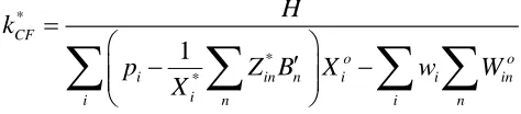
Assume a firm has N=3resources (machines 1, 2 and 3) that produce ˆi =2 products (products 1 and 2). We use ˆC=3 segments to represent the piecewise linearized CFs for each resource. Let X₁ and X₂ represent the number of units of products 1 and 2 to be produced in the period. The parameters of the numerical example are given in Table 3-1 and 3-2.

Table 3-1: Numerical Example Common Coefficients

Product 1 Product 2 Capacity, Cn

kin

Machine 1 3 2 9

Machine 2 5 0 10

Machine 3 0 4 5

Per unit profit, pi 1 0.5 Per unit WIP cost, wi 0.1 0.1

Table 3-2: Clearing Function Segments

Machine 1 Machine 2 Machine 3

Segment 1 2 3 1 2 3 1 2 3

n c

 1 0.4 0 1 0.7 0 1 0.6 0 n

c

 0 2.0 9 0 1.6 10 0 1.6 5

(36)

Figure 3-1: Graph of Clearing Function Segments

Note that for all machines, the intercept of the last segment of the CF, _Cn_ˆ, is equal to its respective Cn in the LP formulation, e.g., ₃1=C1=9. This implies that the maximum throughput of the CF is equal to the capacity limit of the LP at high WIP levels (utilizations).

The classic formulation for a constrained resource linear programming optimization model is:

1 2

Maximize 0.5 Subject to:

X + X

0 2 4 6 8 10 12

0 5 10 15 20

M

ac

h

in

e

H

o

u

rs Used

WIP Hours

3 Machine, 3 Segment Clearing

Function Used in the Paper

Machine 1

Machine 2

(37)

1 2 1

2 1 2

3 2 9

5 10 4 5 , 0 X X X X X X +    

The corresponding model using the clearing functions defined above is:

(

1 2

)

(

11 12 13 21 22 23

)

Maximize 0.5 0.1

Subject to :

X + X − W +W +W +W +W +W

( )( )

( )

( )( )

( )

( )( )

( )

( )( )

( )

( )( )

( )

( )( )

( )

( )( )

( )

( )( )

( )

( )( )

( )

( )( )

( )

( )( )

( )

( )( )

( )

( )( )

( )

1 11 11

1 12 12

1 13 13

2 21 21

2 22 22

2

3 1 3 0

3 0.4 3 2

3 0 3 9

5 1 5 0

5 0.7 5 1.6

5 0 5 10

0 1 0 0

0 0.6 0 1.6

0 0 0 5

2 1 2 0

2 0.4 2 2

2 0 2 9

0 1 0 0

0 0

X W Z

X  +  +  +  +  +  +  +  +  +  +  +  +  + 

( )( )

( )

( )( )

( )

( )( )

( )

( )( )

( )

( )( )

( )

22 22

2 22 22

2 23 23

.7 0 1.6

0 0 0 10

4 1 4 0

4 0.6 4 1.6

4 0 4 5

W Z

X W Z

+  +  +  +  + 11 21 12 22 13 23

1 2 11 12 13 21 22 23 11 12 13 21 22 23

1 1 1

, , , , , , , , , , , , , 0

Z Z

X X W W W W W W Z Z Z Z Z Z

(38)

Using the standard Solver in Microsoft Excel, the optimal values of the main decision variables are identical in both formulations - both formulations yieldX₁*=2 andX₂*=1.25. This congruence of results will, of course, not always occur given different constraints or variable coefficients. Should there be large penalties for WIP, it is natural that the LP model that ignores WIP costs should yield a different result than one that accounts for WIP costs. The optimal objective function value for the LP formulation is G_LP* =2.625and for the CF formulation isG_CF* =1.625. The difference in the objective functions values stems from the additional WIP cost included in the CF formulation. The optimal values of the decision variables in the CF formulation are given in Table 3-3.

Table 3-3: Model Output from CF Formulation Product 1 Product 2 Machine 1 3.889 2.292

*

in

W Machine 2 2.400 0.000 Machine 3 0.000 1.417 Machine 1 0.667 0.333

*

in

Z Machine 2 1.000 0.000 Machine 3 0.000 1.000

*

i

X 2 1.25

Before moving to overhead cost allocation, we can examine the optimal values of the dual variables associated with the capacity constraints in both models. We denote the dual variables of the machines that correspond to constraints in the LP model by_nLP, and those corresponding to the Z constraints in the CF model by CF

n

(39)

Table 3-4: Duels of the Optimal Product Mix for Both the LP and CF Formulation LP

n

 CF

n

 Machine 1 0 0.250 Machine 2 0.200 1.204 Machine 3 0.125 0.171

The result reveals an inherent advantage of the CF model over the LP model in its representation of limited resource capacity. LP duality theory implies that a dual variable will only take a non-zero value when the associated capacity constraint is tight at optimality. In other words, for the LP formulation to yield positive dual prices for capacity, utilization of that resource should be equal to one, implying that there is no benefit to the objective function from adding capacity to resources that are not fully utilized. On the other hand, the CF formulation’s optimal solution frequently results in some of the throughput constraints being tight at optimality (except in cases of degeneracy). In our example, machine 1’s utilization is given by:

( )( ) ( )( )

2 * 1 1 1

1

3 2 2 1.25 8.5

0.94 94%

9 9

i i

k X C

₌



= ₌ + ₌ ₌ ₌

which is less than 100%, suggesting positive slack in the capacity constraints. Hence the optimal LP solution yields ₁LP =0, implying that additional capacity at machine 1 would be of no benefit to the system. On the other hand, as evidenced by the positive dual price

(40)

near-bottleneck machine 1 has a larger dual price than the fully constrained machine 3 (

1 0.250

CF

 = versus ₃CF =0.171).

Another difference between the models is the nonlinear nature of the cost of WIP. Queuing suggests that the average WIP in a queuing system will increase nonlinearly with the utilization. Thus, one would expect the dual price of capacity, the marginal benefit of additional capacity, to increase nonlinearly with utilization, as Kefeli et al. (2011) have shown to be the case. Classical parametric analysis of linear programs shows, in contrast, that for constraints similar to those in our LP formulation, the objective function value is a

piecewise linear function of the right-hand side of the constraint, implying piecewise linear rather than nonlinear benefit of additional capacity. To observe this effect, note in our table of dual values that in the optimal LP solution, each unit of machine 2, which is used exclusively by product 1, is 60% more valuable than machine 3 (₂LP =0.2

and ₃LP =0.125 ) making machine 2 2.2 times more valuable than machine 3 ( 2 2

LP b

 = and 3 0.625

LP b

 = ). In

contrast, in the CF formulation, machine 2 is 7 times as valuable as machine 3 (

2 1.204

CF

(41)

3.2 Where the Kefeli (2011) Model Goes Wrong

Kefeli (2011, Chapter 7) overhead allocation scheme does not generate the same results as this Kaplan-Thompson (1971) application. It is suspected that the dissertation chapter over costs capacity utilization. Kefeli proposes calculating production costs Vin and Vi

based on the following relationships:

1 and

N

in in i n i in

n

V k X V V

=

= =



Kefeli (2011) defines a new variable νi as the relative cost of producing Xi units of

product i to the cost of producing all other products. This relative cost v_i is defined by:

1

ˆ ˆ

1 1 1

N

in i n

i n

i _i _i _N

i in i n

i i n

k X V

v

V k X

  = = = = = =



 

Where 0 ≤ vi ≤ 1. v_i is to represent “the fraction of the total overhead cost allocated to Xi

units of product i.” Thus, given the relative costs vifor each product i, the amount of overhead Hi allocated to product i is given by:

i i

H =Hv

Kefeli (2011) invokes the strong duality theorem of LP optimality to introduce the heart of where the analysis goes awry. While it is true “that in an optimal solution, the optimal values of the primal and dual problems will be equal, implying that marginal profit should equal marginal cost at optimality,” the following formula is incorrect:

1

N

in i n i i n

k X p X

=

(42)

The real relationship between the primal and dual at optimality is pX*_{= ω}*_{b. By}

simple algebra substitution, the Kefeli (2011) dissertation model seems to assert that at

optimality,

1

N in i n

k X b

=



which is clearly not the case for this example. The transpose of the

b vector in this case is (0,…,0,1,1,1), not the sum of machine times kin multiplied by the

number of Xi produced. It is no surprise, then, that the model fails to maintain the optimal

product mix for many of the problems where this method has been applied.

3.3 Allocating Untraceable Overhead

Having solved the mathematical models to optimality and calculated the dual variables associated with the production resources, we now proceed to cost allocation. We assume that we have H =1 units of total untraceable overhead cost to allocate to our optimal product mix of 2 units of product 1 and 1.25 units of product 2. Following Kaplan and Thompson’s (1971) Rule 1 for allocating untraceable overhead, we define the ratio of overhead costs to variable contribution

* * *

* where

H

k G px b

G 

= = =

obtaining

1 8

0.381 2.625 21

LP

k = =

and

1

0.615 1.625

CF k =

(43)

can only absorb G units. The difference in variable contributions is due to the CF model’s explicit representation of WIP holding costs, which are omitted in the LP model. To allocate the one unit of untraceable overhead, the coefficients are changed using k so the new

objective function is, using matrix notation,

(

*

)

Maximize p−k A x Due to complimentary slackness at optimality, either ω*_A

j = pj or xj = 0 for each column j in

matrix A. Our equation can thus be rewritten, after some algebra,

(

)

Maximize 1−k px

We can calculate the new coefficients of the objective function of the LP formulation as follows:

( )

1 2

8 13 8 13

1 1 , 1 (0.5)

21 21 21 42

p = −_ _ = p = −_ _ =

   

The LP objective function that allocates untraceable overhead according to Rule 1 is thus:

1 2

13 13 Maximize

21X +42X

subject to the same equations for the basic LP problem as in section 3.1. Likewise, we can use the same methodology to calculate the new objective function for the CF:

(

)( )

(

)

(

)

1 1 0.615 1 0.385, 2 1 0.615 (0.5) 0.1925, wi 1 0.615 ( 0.1) 0.0385

p = − = p = − = = − − = −

Therefore, we get:

(

)

1 2 11 12 13 21 22 23

Maximize 0.385X +0.1925X −0.0385 W +W +W +W +W +W

(44)

Proof: The decision variables remain unchanged because both the feasible regions are unchanged, and the new objective functions are parallel to the original objective functions. This is clearly shown by the equation above where the new objective functions are the old objective functions scaled by the constant (1 - k).

The LP formulation now shows a net profit of 1.625 and the CF formulation 0.625, each reflective of the one unit of untraceable overhead allocated between X1 and X2. Kaplan and

Thompson show that the amount of fixed overhead applied to each unit of production of the LP formulation is kLPω*A.

*

3 2

8 1 1 8 4

0 5 0

21 5 8 21 21

0 4 LP

k  A

 

    

= _ __ _=_ _

 _ _  

 

Multiplying by the optimal values of x from the primal, we obtain the total fixed overhead absorbed by each product: ₁ = 8

( )

2 16, ₂ = 4 5 5

21 21 21 4 21

X = X  _{ }=

 

which, of course, sum to one unit.

Before allocating fixed overhead for the CF formulation, we must first recognize that the dual variables from the LP formulation are different from the dual variables for the CF formulation. Recall that from strong duality,

* *

px =b

where px* is the profit vector per unit (contribution margin) multiplied by the total units of each product produced at optimality. The right-hand side, ω*_{b is the value of capacity at}

(45)

0.125. We can calculate the value of capacity from the original LP formulation by

multiplying 0.20 by 10 units of the machine 2 used plus 0.125 times 5 units of the machine 3 used. Not surprisingly, the value of capacity equals the planned profit of 2.625.

The duals of the CF formulation represent something different. These duals are the value of capacity for each of the machines, not on a per unit basis. A nice feature of the CF formulation is that the equations of the primal problem can be rearranged such that only the Zin variable constraints have nonzero right-hand side values (which happen to be 1) for the b

vector. Another nice feature is that the only interdependencies of the products are in the Zin

variable constraints. Therefore, the value of capacity is simply ω*_b=ω*_{for this CF}

formulation. We can allocate fixed untraceable overhead to products by allocating overhead based on each machine’s capacity value and the percentage of capacity value generated by each product. Because the only equations that intermingle the products are the Zin decision

variables and that the columns on the A matrix representing these Zin variables are trivial, we

take advantage of symmetry in the A matrix with respect to the Zin variables and apply

kCFω*A to get the overhead allocated to each machine.

(

)









*

1 0 0 1 0 0 0.615 0.25 1.204 0.171 0 1 0 0 1 0 0 0 1 0 0 1 0.154 0.741 0.105 0.154 0.741 0.105 CF

k  A

 

 

= _ _=

 

 

We multiply the overhead allocated to each machine by the Zin decision variables assigned to

(46)









1

2

2 3

Fixed overhead allocated to 0.154 0.741 0.105 1 0.844

0

1 3

Fixed overhead allocated to 0.154 0.741 0.105 0 0.156

1 X X     = _ _=         = _{ }=    

Because kCFω*Ax* = kCFω*b at optimality, we can further simplify our method. For the CF

formulation, because b = 1, when there are no product sales or production interdependencies the calculation simplifies to

*

Fixed overhead allocated to product _i _CF _in _nCF n

X =k



Z 

where the Zin variables show the proportion of machine n overhead to be applied to each

product i. Returning to our numerical example, we see that

(

) ( )(

)

(

) ( )(

)

1 2

2

total fixed overhead absorbed = 0.615 0.250 1 1.204 0 0.171 0.843 3

1

total fixed overhead absorbed = 0.615 0.250 0 1.204 1 0.171 0.156 3 X X   ₊ ₊ _   _{ }      ₊ ₊ _   _{ }   

which is only slightly different to our previous result due to rounding errors. Notice this overhead allocation can proceed directly from the initial problem.

Another way to allocate the amount of fixed overhead applied to each product is to recognize that the overhead applied to each product is the per unit overhead applied

multiplied by the number of units produced at optimality, or kω*_Ax*_{. Due to complementary}

slackness at optimality, the equation is reduced to simply kpx*. For the LP formulation,

( )( )

( )

1 2

8 16

total fixed overhead absorbed = 1 2

21 21

8 5 5

total fixed overhead absorbed = 0.5

21 4 21

(47)

Calculating the overhead allocated to each product in the CF formulation is more complicated. There is a key distinction between the LP and CF results – the new CF

formulation scales the coefficients of WIP charges by (1 - kCF). However, a closer look at the

results of the new CF formulation shows that throughput is reduced by 1.615 units while the total WIP charges due to scaling are reduced by 0.615 units. Subtracting the difference, we are left with the 1 unit of fixed untraceable overhead that we allocated to products X1 and X2.

The missing WIP charges are fully accounted for in the equivalent lost throughput of the new formulation. Recall that in our CF formulation, WIP levels are objective function decision variables. We can determine how the fixed overhead is allocated to products using a slightly more complex procedure.

* *

Overhead absorbed by product _i _CF _i _i _i _in n

X =k _p X − wW _







Numerically in our example, the overhead absorbed by each product is calculated as follows:

( )( ) ( )(

)

(

)

( )(

) ( )(

)

(

)

1 2

total fixed overhead absorbed = 0.615 1 2 0.1 3.889 2.400 0 0.843

total fixed overhead absorbed = 0.615 0.5 1.25 0.1 2.292 0 1.417 0.156

X X

− + + 

Notice this overhead allocation also can proceed directly from the initial problem. There is no need to set up the second CF linear program to determine overhead allocation. One just needs the results of the first CF formulation.

3.4 Allocating Traceable Overhead

(48)

reduced below zero, the solution to either formulation will no longer remain optimal. (In fact, the dual’s problem structure explicitly forbids this.) If a machine’s marginal contribution becomes negative, the solution would redirect the production mix to favor products using machines that have positive contribution, baring interdependencies of the demand for each product.

Kaplan Thompson Rule 2 allocates overhead that can be traced directly to resources among the products. The traceable overhead assigned to a resource n is divided by the amount of the resource quantity bn and assigned to variable Bn. The traceable overhead is

then applied to the resource using the following rule:

*

* *

such that , assign a traceable overhead charge of

n n n n

n B B B

n B B



 



  =



  =

The new objective function, in matrix notation, is

(

)

Maximize p−B A x

This rule enforces nonnegative duals by limiting the amount of traceable overhead that can be applied to any resource. Any remaining traceable overhead is added to the pool of untraceable overhead which is then allocated by Rule 1. To apply Rule 1, Kaplan and Thompson define a new ratio of overhead costs to variable contribution, k*_{using the}

following:

(

)

*

LP

H k

p B A x =

 −

(49)

(

)

*

LP

H k

B b 

=

 −

Notice that the denominator stays positive based on Rule 2. The combined objective function in matrix notation, after some algebra, is

(

)

(

)

(

*

)

Maximize p−B A 1−k_LP x

The CF version will be different. Recall that the duals in the CF formulation represent the total marginal value of the resource, not the marginal value per unit of additional

capacity. Therefore, Bn is now the total traceable overhead to be applied to a resource, not the

per unit overhead. The Bʹ ‘s are still calculated by Rule 2. For Rule 1, we were able to use the relationship ω*_{A = p to calculate the new coefficients of the objective function. For Rule 2, it}

is unclear what corresponds to BʹA in the CF formulation. Recall that the dual variables from the CF formulation are associated with the Zin constraints which allocate the time used by

product i on resource n. If we apply the traceable overhead based on the Zin variables, we still

have a problem. We need to use the results of the initial CF formulation to determine the new coefficients of the new objective function. WIP charges are still a function of resource usage based on the product mix. Leaving the product decision variables free to recalculate, the revised objective function for the CF model is then

* *

1

Maximize _i _in _n _i _i _in

i i n i n

p Z B X w W

X

 _

− −

 

 



 

(50)

formulation recalculates, the original optimal values are marked with *_{and the new optimal}

values are marked with o.

* * * 1 CF o o

i in n i i in

i

i n i n

H k

p Z B X w W

X =    − −      



 

Using the remaining capacity value is an easier way to calculate k*CF. WIP is already “baked

into” the duals and the b parameters are all equal to 1, yielding:

(

)

* * CF n n n H k B  =  −



Finally, the objective function with the combined traceable and untraceable overhead is

(

)

(

)

* * *

*

1

Maximize _i _in _n 1 _CF _i _i 1 _CF _in

i i n i n

p Z B k X w k W

X  _ − − − −    



Returning to the numerical example, instead of allocating untraceable overhead as before, it is determined that the overhead is really fixed and assignable to each machine. Recall our dual variables at optimality and calculate the capacity value for each machine reprinted in Table 3-5.

Table 3-5: Contribution Margin of the Optimal Product Mix for Both LP and CF Model LP

n b

 CF( 1) n b

 =

Machine 1 0 0.250

Machine 2 2.000 1.204 Machine 3 0.625 0.171

(51)

model, we should see that both formulations are able to allocate the traceable overhead to the products that use machine 2 and that the optimal product mix is maintained.

Let’s begin with the LP formulation. 1/b2 = 0.1 = B2ʹ. Recall we get A from our

machine constraints:

1 2

3 2 9 Machine 1 constraint 5 10 Machine 2 constraint

4 5 Machine 3 constraint

X X

+ 

 

Note that only product 1 gets produced by machine 2. So, for the LP formulation, our new objective function is calculated by

( )

1 2

for X → −1 0.1 5 =0.5, for X →0.5 0.1(0)− =0.5 Our new objective function for the LP formulation is thus

1 2

Maximize 0.5X +0.5X

subject to the machine capacity constraints and nonnegative values for our decision variables constraints. The new value of the objective function is 1.625 and the values of X1 and X2

remain 2 and 1.25 respectfully. The new duals are ωo

1 = 0, ωo2 = 0.1, and ωo3 = 0.125. The

overhead absorbed is

( )

(

)

( )

(

)

1 1

2 2

total fixed overhead absorbed = 0.1 5 2 1 total fixed overhead absorbed = 0.1 0 1.25 0

o

X B A X

 =  =

using the product contribution margin. Knowing that all of the overhead of machine 2 gets absorbed by only product 1, the overhead absorbed by product 1 can be calculated as just Bʹb, or the difference ω*2b - ωo2b = 0.2(10) – (0.1) (10) = 1.

(52)

( )( )

*

1 1 * 2 12

1 *

2 2 * 2 22

2

1 1

coefficient for 1 1 1 0.5

2

1 1

coefficient for 0.5 1 0 0.5

1.25

X p B Z

X

X p B Z

X  _ _{ }  →_ − _{ }= − _=      _ _{ } _ →_ − _{ }= − _=    

Noting that the WIP variables are unchanged, the new objective function is thus:

(

)

1 2 11 12 13 21 22 23

Maximize 0.5X +0.5X −0.1W +W +W +W +W +W

subject to constraints in equations machine clearing function constraints, the Z constraints, and the nonnegativity constraints. The results in this case are predictable. The decision variables all remain unchanged with the new objective function value of 0.625, one unit less than the original CF formulation. The new duals are ωo

1 = 0.250, ωo2 = 0.204, and ωo3 =

0.171. The total traceable overhead absorbed can be calculated as

( )( )

*

1 * 2 12 1

1 *

2 * 2 22 2

2

1 1

total fixed overhead absorbed = 1 1 2 1 2

1 1

total fixed overhead absorbed = 1 0 1.25 0 1.25

o

X B Z X

X

X B Z X

X  _  ₌  ₌   _ _    _  ₌  ₌   _ _  

or using the duals, given that the decision variables remain unchanged, by

(

)

(

)

(

)

(

)

(

) (

)

(

)

(

)

(

)

(

)

* * * * * *

1 1 1 11 2 2 12 3 3 13

* * * * * *

2 1 1 21 2 2 22 3 3 23

total fixed overhead absorbed = + 2

0.250 0.250 1.204 0.204 1 0.171 0.171 0 1 3

total fixed overhead absorbed = + 1

0.250 0.250 1.20 3

o o o

X Z Z Z

     

− − + −

= − + − + − =

− − + −

= − +

(

4 0.204 0−

) (

+ 0.171 0.171 1 0−

)

=

(53)

traceable overhead (which is 1.625). Therefore, k*

LP = 16/65. We use this result and equation

(29) to calculate the new coefficients

( )

(

)

(

)

1 1 2 2 16 49

coefficient for 1 0.1 5 1

65 130

16 49

coefficient for 0.5 0.1(0) 1

65 130 X p X p   _ → − _ − _= =     _ → − _ − _= =  

Our new objective function for this combined LP formulation is thus

1 2

49 49 Maximize

130X +130X

subject again to the machine capacity constraints and product nonnegativity constraints. The new value of the objective function is 1.225 and the values of X1 and X2 remain 2 and 1.25

respectfully. The total fixed overhead absorbed by product, both traceable and untraceable, is

(

)

(

)

1 1 1 1

2 2 2 2

49 81

total fixed overhead absorbed = 1 2 1.246

130 65

49 2

total fixed overhead absorbed = 0.5 1.25 0.154

130 13

o

X p p X

   − = −_ _ = =      − =_ − _ = =  

using the product contribution margins.

Allocating 0.4 units of untraceable overhead in addition to the 1 unit of traceable overhead for the CF formulation first requires the calculation of a newk*CF. Recall the value

of the objective function after allocating the traceable overhead in the CF formulation is 0.625. Therefore, k*

CF = 0.4/0.625 = 0.64. We calculate the coefficients in the objective

function by using our equation and our newly calculated k*CF

(

)

( )( ) (

)

(

)

( )( ) (

)

( )

(

)

( )(

)

* *

1 1 * 2 12

1

* *

2 2 * 2 22

2 *

1 1

coefficient for 1 1 1 1 1 0.64 0.18

2

1 1

coefficient for 1 0.5 1 0 1 0.64 0.18

1.25 coefficient for w 1 0.1 1 0.64 0.036

CF

i i CF

X p B Z k

X

X p B Z k

Extending the Kingman General Arrival, General Service Queuing Approximation to Overhead Allocation and Service Pricing.

DEDICATION

BIOGRAPHY

ACKNOWLEDGMENTS

TABLE OF CONTENTS

LIST OF TABLES

LIST OF FIGURES

CHAPTER 1:

Introduction

WIP M/M/1

CHAPTER 2:

Previous Related Work

2.1

Accounting Research

2.2

Linear Programming Research

2.3

Medical Applications

CHAPTER 3:

Overhead Allocation Using Clearing Functions

3.1

Overhead Allocation Using Traditional Clearing Function Formulation

3 Machine, 3 Segment Clearing

Function Used in the Paper

(

)

(

)

( )( )

( )

( )( )

( )

( )( )

( )

( )( )

( )

( )( )

( )

( )( )

( )

( )( )

( )

( )( )

( )

( )( )

( )

( )( )

( )

( )( )

( )

( )( )

( )

( )( )

( )

( )( )

( )

( )( )

( )

( )( )

( )

( )( )

( )

( )( )

( )



3.2

Where the Kefeli (2011) Model Goes Wrong





 



3.3

Allocating Untraceable Overhead

(

)

(

)

( )

(

)( )