Experimental and simulation Studies of a Two Seater Light Aircraft

Experimental and simulation Studies of a Two Seater Light

Aircraft

Iskandar Shah Ishak, Shabudin Mat,Tholudin Mat Lazim, Mohd. Khir Muhammad, Shuhaimi Mansor, Mohd Zailani Awang

Department Aeronautics and Automotive, Faculty of Mechanical Engineering,

Universiti Teknologi Malaysia, 81310, UTM Skudai, Johor,

Malaysia.

Abstract: This paper presents the aerodynamic studies carried out on a three-dimensional aircraft model. The test model is a 15%

scaled down from a two-seater light aircraft that close to the Malaysian made SME MD3-160 aircraft. The aircraft model is equipped with control surfaces such as flaps, aileron, rudder and elevator and it is designed for pressure measurement testing and direct force measurement using a 6-components balance system. This aircraft model has been tested at two different low speed tunnels, at Universiti Teknologi Malaysia tunnel sized 1.5 x 2.0 meter2 _{test section, and at Institute Aerodynamic Research, National Research} Council of Canada sized 3 x 2 meter2 _{tunnel. The speed during testing at UTM and IAR/NRC tunnels was up to 70 meter/second,} which is corresponds to Reynolds numbers of 1.3 x 106.The longitudinal and lateral directional aerodynamic characteristics of the aircraft such as coefficients of pressure, forces (lift, drag, side) and moments (roll, pitch and yaw) have been experimentally measured either using direct force measurement or pressure measurement method. The data reduction methods include the strut support interference factor using dummy image and the blockage correction have been applied in this project. The results showed that for the undeployed flap configuration, the stalling angle of this aircraft is 160 _{at C}

LMax = 1.05 measured by UTM - LST, compared to CLMax =1.09 at stalling angle 150 _{by IAR- NRC. Beside the experimental study, simulation also be performed by using a commercial} Computational Fluid Dynamics (CFD) code, FLUENT Version 5.3. Experimental works at UTM and IAR – NRC tunnel show that the aerodynamic characteristics of this light aircraft are in a good agreement with each other. Simultaneously, the aerodynamic forces obtained from experimental works and CFD simulations have been compared. The results proved that they are agreeable especially at a low angle of attack.

1.0 INTRODUCTION

Nowadays, the implementation of wind tunnel testing and simulation by CFD is a must in the stage of the design analysis process. This paper will present the wind tunnel testing technique on a 15% scaled-down model of two-seater light aircraft and the data reduction procedures. CFD simulation also is carried out for comparison purposes.

2.0 EXPERIMENTAL STUDY

A 15% scaled down model of two-seater light aircraft that close to the Malaysian made SME MD3-160 has been selected for the experiment. The testing was previously conducted at IAR/NRC (in Spring of 2000) and later at UTM-LST (in October 2002). For the data reduction, corrections have been made for wind tunnel flow angularity (including balance

misalignment), blockage, buoyancy,wall interference and STI (Strut, Tare and Interference) corrections. The following

discussion is based on the testing conducted at UTM-LST.

2.1 Wind Tunnel Flow Angularity Correction

This correction is to remove the effects of the wind tunnel flow angularity (upwash) and any misalignment between the balance lift vector and the free stream. In order to assess these effects, a model is run upright and inverted with main

struts and dummy struts installed. The two runs are over plotted and the corrections to

α

ideal tunnel, the two runs should overlay each other.

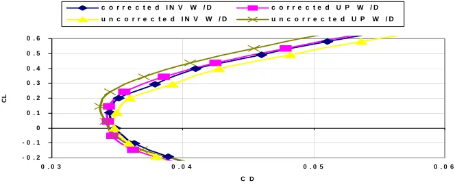
Fig. 2: Results from Upright and Inverted Pitch Runs, Main Dummies Installed

These two curves are parallel but offset by 0.52o_{. As shown in Barlow, the correction is equal to half of the angle offset}

which is 0.26o_{. Therefore the model-upright data needs to have 0.26}o _{added to the incidence angle and the model-inverted}

data needs to have 0.26o _subtracted.

The measured drag also needs to be corrected. This arises because the non-orthogonality of the lift vector to the flow means that a small component of the measured lift is actually drag. A shown in Barlow, the additive correction to drag coefficient for an upright model is ∆CD = CL * tan (

α

α

Fig.3: Implementation of Flow UpWash Correction to Drag Polar

2.2 Blockage Correction

In preparation for removal of blockage and buoyancy effects, the data are converted to wind axis. Lift and yawing

moment are unchanged. With the subscripts W for wind axis and S for stability axis, and ψ defined as positive to the

right when viewed from above, the remaining equations are:

CYW = CYS cosψ - CDS sinψ CDW = CDS cosψ + CYS sinψ

- 0 .2 - 0 .1 0 0 .1 0 .2 0 .3 0 .4 0 .5 0 .6

- 5 - 4 - 3 - 2 - 1 0 1 2 3 4 5

a lp h a ( d e g )

CL

u n c o r r e c t e d IN V W /D u n c o r r e c t e d U P W /D

- 0 . 2 - 0 . 1 0 0 . 1 0 . 2 0 . 3 0 . 4 0 . 5 0 . 6

0 . 0 3 0 . 0 4 0 . 0 5 0 . 0 6

C D

CL

CmW = CmS cosψ + ClS sinψ*(b/c) ClW = ClS cosψ - CmS sinψ*(c/b)

The premise of the corrections is based on a perturbation velocity

ε

determined from the uncorrected velocity, VU, as follows

VC = VU*(1+ ε) where ε = εsb + εwb

εsb = Solid blockage

εwb = Wake blockage

The rest of the equations are :

qc = qu [1 + (2 – M2) ε] Mc = Mu [1 + (1 + 0.2 M2) ε] Tc = Tu (1 – 0.4M2ε)

Pc = Pu (1-1.4M2ε)

ρc = ρu (1 – M2ε)

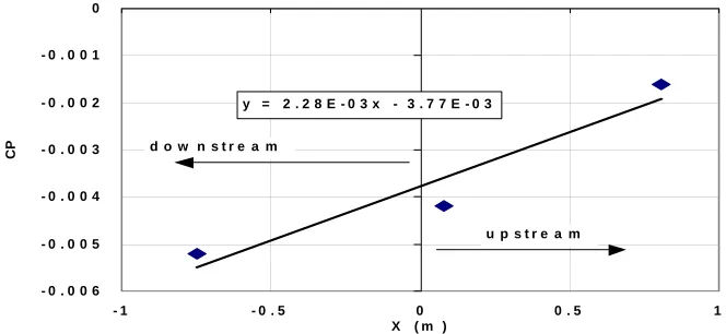
2.3 Buoyancy Correction

Before correcting the aerodynamic loads due to the effects of blockage, any buoyancy effects are removed from the wind axis drag.

Fig. 4: Static Pressure Gradient in Empty Test Section of UTM-LST

The buoyancy can be expressed as :

∆CD = dCp/dx*(V/S) where S is the wing area and V is the fuselage volume

It is found that the buoyancy correction for the model under test is only about 1 drag count (∆CD = 0.0001).

With the completion of the corrections which are wind-axes based, the results can be transformed back to stability axes as follows (CL and Cn are unchanged) :

CYS = CYW cosψ + CDW sinψ CDS = CDW cosψ - CYW sinψ CmS = CmW cosψ - ClW sinψ*(b/c) ClS = ClW cosψ + CmW sinψ*(c/b)

y = 2 . 2 8 E - 0 3 x - 3 . 7 7 E - 0 3

- 0 . 0 0 6 - 0 . 0 0 5 - 0 . 0 0 4 - 0 . 0 0 3 - 0 . 0 0 2 - 0 . 0 0 1 0

- 1 - 0 . 5 0 0 . 5 1

X ( m )

CP

2.4 Corrections for Wall Interference

These corrections typically represent some of the largest corrections applied to 3D aircraft models. The corrections arise because of the reflection of the wing tip vortices in the tunnel walls, floor and ceiling.

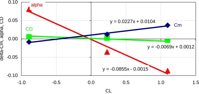
2.5 STI Corrections

The STI correction are applied as the final correction of this data reduction. Data for STI were collected for a pitch run

only at α= -15°, 0° and +15° owing to current UTM-LST limitations.

y = -0.0855x - 0.0015

y = -0.0069x + 0.0012 y = 0.0227x + 0.0104

-0.10 -0.05 0.00 0.05 0.10

-1.0 -0.5 0.0 0.5 1.0 1.5

CL

de

lt

a-C

m

, a

lpha

,

C

D

alpha

CD Cm

Fig. 5: STI Corrections

STI corrections as developed by subtracting “all dummy inverted” data from “no dummy inverted” data that will need to be subtracted from “no dummy upright” data.

3.0 CFD SIMULATION

For a comparison purpose, simulation is done at a grace of a commercial CFD code, Fluent 5.3. A simplified 15% scaled

model is simulated at 1.3 x 106 _{Reynolds number and the speed is increased from 60 to 70 m/s. In this project, the}

simulations were carried out at two different number of elements, angle of attack varies from 00_{, 5}0_{, 10}0 _{and 15}0 _with

using k-epsilon standard. First simulation, the model was simulated at 230 000 elements and second simulation was at 300 000 elements. Results for both simulations were then compared for a validation purposes. This is to ensure that the aerodynamic forces obtained from this study are free from the elements factor. Figure 6 gives a comparison results for both simulations.

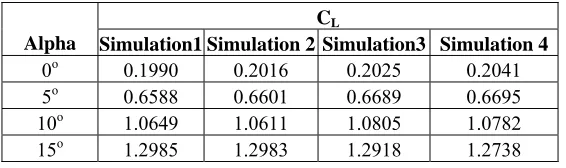
CL

Alpha Simulation1 Simulation 2

0o _{0.1990 0.2016}

5o _{0.6588 0.6601}

10o _{1.0649 1.0611}

CFD Simulation for CL

0.0 0.5 1.0 1.5

0 5 10 15 20

Alpha (Deg)

CL

Simulation at 300 000 Simulation at 230 000

Fig. 6: CFD Simulation for CL

From figure 6, it can be seen that the lift coefficient is increased with the increase of angle of attack. There are only about

1% deviation comparatively between this two simulations. Figure 7 shows an example of simulations at 150 _{and 0}0 _angles

of attack at 230 000 meshing elements.

Fig. 7: Simulation study at 150 _{and 0}0 _{angle of attack.}

Beside the simulation with k-epsilon standard, the simulation also be done at k-epsilon RNG. Figure 8 shows a comparison of the lift coefficient for k-epsilon standard and k-epsilon RNG. Simulation 1 and 2 represent the lift coefficient for epsilon with 230 000 and 300 000 elements respectively whereas simulation 3 and 4 is the results for k-epsilon RNG with respects to the same amount of elements. Figure 8 shows that the lift coefficient is increased in average by using k-epsilon RNG compared to the k-epsilon standard and obvious at low angle of attack. Since the difference is merely small, the results can be accepted.

CL

Alpha Simulation1 Simulation 2 Simulation3 Simulation 4

0o _{0.1990 0.2016 0.2025 0.2041}

5o _{0.6588 0.6601 0.6689 0.6695}

10o _{1.0649 1.0611 1.0805 1.0782}

15o _{1.2985 1.2983 1.2918 1.2738}

Fig. 8: Lift Coefficients for k-epsilon and k-epsilon RNG.

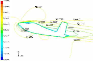
The wing and fuselage velocity profile are then analysed, simulation result at the speed of 70 m/s and angle of attack of

50 _{is discussed. Figure 9 shows a velocity profile on the wing. The highest speed on wing is 90.97 m/s achieved on the}

Fig. 9: Velocity profile on wing

Figure 10 is the velocity profile on the centre of the fuselage at 70 m/s simulation. From this simulation it is found that the speed at the bottom front of this aircraft is only about 58 m/s. The speed behind the aircraft is merely around 48.16 m/s, this is might caused by the flow has been saturated and vortex flow has been generated at this particular location.

Fig. 10: Velocity profile on fuselage

4.0 RESULTS

Figure 11 shows a comparison results for the lift coefficient obtained from both studies in this project. Experimental

study at IAR – NRC showed that this aircraft stalled at 150_{angle of attack and equivalent to C}

lmax of 1.09, whereas Clmax is

found to be 1.05 measured by UTM-LST at angle of attack 160_{. The coefficient of lift is found slightly higher by CFD}

study. For example at 150_{, CFD depicts the coefficient of lift is about 1.29}o _{whereas IAR/NRC and UTM – LST show}

only 1.09o _{and 1.04}o _{respectively. However, the slopes are agreeable by each other.}

CL

Alpha IAR - NRC UTM-LST Simulation1 Simulation 2 Simulation3 Simulation 4

0o _{0.24 0.17 0.1990 0.2016 0.2025 0.2041}

5o _{0.64 0.58 0.6588 0.6601 0.6689 0.6695}

10o _{0.92 0.88 1.0649 1.0611 1.0805 1.0782}

CL Versus Angle of Attack

0 0.2 0.4 0.6 0.8 1 1.2 1.4

0 2 4 6 8 10 12 14 16

Angle of Attack

CL

IAR-NRC UTM-LST SIMULATION 1 SIMULATION 2

Fig. 11: Profile of Lift Coefficient

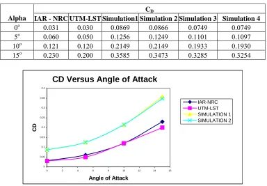
Figure 12 shows the profile of drag coefficient of this aircraft. From the experiment study at IAR/NRC, the drag

coefficient is 0.23 compared to 0.2 measured by UTM-LST at 150_{angle of attack. This shows that the drag measured by}

both tunnels is agreeable each other at low angle of attack. Figure 12 also depicts that the drag coefficient is slightly

higher by CFD study compared to the experimental works. For example at zero angle of attack, CD obtained by CFD is

around 0.08 compared to 0.03 from the experiment. This small deviation may due to the inaccuracy and imperfection of the CFD model.

CD

Alpha IAR - NRC UTM-LST Simulation1 Simulation 2 Simulation 3 Simulation 4

0o _{0.031 0.030 0.0869 0.0866 0.0749 0.0749}

5o _{0.060 0.050 0.1256 0.1249 0.1101 0.1097}

10o _{0.121 0.120 0.2149 0.2149 0.1933 0.1930}

15o _{0.230 0.200 0.3585 0.3473 0.3285 0.3254}

CD Versus Angle of Attack

0 0.05 0.1 0.15 0.2 0.25 0.3 0.35 0.4

0 2 4 6 8 10 12 14 16

Angle of Attack

CD

IAR-NRC UTM-LST SIMULATION 1 SIMULATION 2

Fig. 12: Profile of Drag Coefficient

5.0 RECOMMENDATION

digitising the scan image of aircraft model using a software called Photomodeller Pro 3.0 might be advantageous. By this, it is hope that a real image of the aircraft model will be obtained.

6.0 CONCLUSION

Throughout this paper, the procedures and result of the experimental and simulation studies have been presented. Results for the lift coefficient show that both studies are in well agreement especially at a low angle of attack. Nevertheless, CFD simulation shows that the drag coefficient is slightly higher than experimental. For the STI Corrections, in future gathering data at a few intermediate angles (+ve and –ve) might be advantageous.

7.0 ACKNOWLEDGEMENT:

1) Institute Aerodynamic Research, National Research Council, IAR – NRC, Ottawa, Canada.

2) SME Aerospace, Kuala Lumpur, Malaysia.

8.0 REFERENCES:

[1]Barlow J.B., et al (1999), “Low Speed Wind Tunnel Testing” 3rd edition, New York: A Wiley – Interscience Publication.

[2] Alan Pope, M.S. (1954), “ Wind Tunnel Testing.” 2nd Edition, New Jersey – PrenticeHall.

[3] Katz,J. and Plotkin, A. (1991). “Low Speed Aerodynamic from wing Theory To Panel Methods.” New

York:McGraw Hill Inc

[4] Anderson, John D. (1995). “Computational Fluid Dynamics – The Basics with Applications”. New

York:McGraw Hill Inc.

[5] Singhal, A.K. ( 1998 ). “Key Elements of Verification and Validation of CFD Software.” Hustville,

AL : CFD Research Corporation.