University of Windsor University of Windsor
Scholarship at UWindsor
Scholarship at UWindsor
Electronic Theses and Dissertations Theses, Dissertations, and Major Papers
1-15-2016
Mathematical Modelling and a Meta-heuristic for Cross Border
Mathematical Modelling and a Meta-heuristic for Cross Border
Supply Chain Network of Re-configurable Facilities
Supply Chain Network of Re-configurable Facilities
SAGAR MANOHAR HEDAOO University of Windsor
Follow this and additional works at: https://scholar.uwindsor.ca/etd
Recommended Citation Recommended Citation
HEDAOO, SAGAR MANOHAR, "Mathematical Modelling and a Meta-heuristic for Cross Border Supply Chain Network of Re-configurable Facilities" (2016). Electronic Theses and Dissertations. 5640.
https://scholar.uwindsor.ca/etd/5640
This online database contains the full-text of PhD dissertations and Masters’ theses of University of Windsor students from 1954 forward. These documents are made available for personal study and research purposes only, in accordance with the Canadian Copyright Act and the Creative Commons license—CC BY-NC-ND (Attribution, Non-Commercial, No Derivative Works). Under this license, works must always be attributed to the copyright holder (original author), cannot be used for any commercial purposes, and may not be altered. Any other use would require the permission of the copyright holder. Students may inquire about withdrawing their dissertation and/or thesis from this database. For additional inquiries, please contact the repository administrator via email
Mathematical Modelling and a Meta-heuristic for Cross
Border Supply Chain Network of Re-configurable
Facilities
By
SAGAR MANOHAR HEDAOO
A Thesis
Submitted to the Faculty of Graduate Studies
through the Department of Industrial and Manufacturing Systems Engineering
in Partial Fulfillment of the Requirements for the
Degree of Master of Applied Science
at the University of Windsor
Windsor, Ontario, Canada
2015
Mathematical Modelling and a Meta-heuristic for Cross
Border Supply Chain Network of Re-configurable
Facilities
By
SAGAR MANOHAR HEDAOO
APPROVED BY:
G. Pandher
Odette School of Business
Z. Pasek
Industrial & Manufacturing Systems Engineering Department
F. Baki (Co-supervisor)
Odette School of Business and Industrial & Manufacturing Systems Engineering Department
A. Azab (Co-supervisor)
Industrial & Manufacturing Systems Engineering Department
iii
Author’s Declaration of Originality
I hereby certify that I am the sole author of this thesis and that no part of this thesis has
been published or submitted for publication.
I certify that, to the best of my knowledge, my thesis does not infringe upon anyone’s
copyright nor violate any proprietary rights and that any ideas, techniques, quotations, or any
other material from the work of other people included in my thesis, published or otherwise, are
fully acknowledged in accordance with the standard referencing practices. Furthermore, to the
extent that I have included copyrighted material that surpasses the bounds of fair dealing within
the meaning of the Canada Copyright Act, I certify that I have obtained a written permission from
the copyright owner(s) to include such material(s) in my thesis and have included copies of such
copyright clearances to my appendix.
iv
Abstract
In supply chain management (SCM), Facility location-allocation problem (FLAP)
comes under strategic planning and has been a well-established research area
within Operations Research (OR).
Owing to the billion dollar trade between USA-Canada the supply chain costs and
difficulties are growing. Binary Integer Linear Programming (BILP) mathematical
model is formulated to incorporate several parameters which would optimize the
overall supply chain cost.
Capacitated, single commodity, multiple time period
(dynamic) and multi-facility location allocation problem is considered. Canada being
a part of “The Kyoto protocol”, a part of the United Nations Framework
Convention on Climate Change, has declared to abide by global effort to reduce
GHG emissions. Developed math model will include an important constraint to
optimize production keeping the Carbon di-oxide gas [
𝑐𝑜
2] emission levels within
specified limits. Simulated annealing based Meta-heuristic is developed to solve the
problem to near optimality.
v
Dedication
Firstly, dedicated to my respected father, Mr. Manohar Hedaoo, who has always
been a silent supporter to my entire family.
Secondly, to my mother, Mrs. Madhulika Hedaoo, a creative and strong minded
women, who taught me, “Impossible is nothing”
vi
Acknowledgement
First and foremost, I would like to thank my supervisors, Dr. Fazle Baki and Dr. Ahmed Azab for giving me an opportunity to complete my Master of Applied science in Industrial Engineering at University of Windsor. I would like to thank my committee members Dr. Gurupdesh Pandher and Dr. Zbignew Pasek for their valuable inputs towards my thesis.
I would like to thank Dr. Walid Abdul-Kader, Dr. Michael Wang, Dr. Guoqing Zhang and Professor. Razavi Far whose courses helped me shape my career.
I would like to thank Dr. Z. Pasek for appointing me at various GA positions. I would like to extend my thanks to all faculty members at University of Windsor, who directly or indirectly helped me. Thank you to Qin Tu, IMSE department secretary, for all support.
Thank you to my loving sister Madhuja Lanke and her spouse Amol Lanke for all their encouragement.
In addition to my parents and my supervisors, thank you to my uncle Atul Madiwale for his generous financial support.
vii
Table of Contents
Author’s Declaration of Originality ... iii
Abstract ... iv
Dedication ... v
Acknowledgement ... vi
List of Figures ... ix
List of Tables ... x
Abbreviations ... xi
1 Introduction ... 1
1.1 Brief Introduction ... 1
1.2 Statistical Background ... 2
1.3 Motivation ... 4
1.4 Research Objectives ... 6
1.5 Problem and Thesis Statement ... 6
1.6 Research Approach ... 7
2 Literature review ... 8
2.1 Supply Chain Network Design Literature Review ... 9
2.2 Emission Literature Review ... 18
2.3 Research Contribution ... 22
3 Methodology ... 23
3.1 Problem Description ... 23
3.2 Assumptions ... 25
3.3 Parameters ... 26
3.4 Indices ... 27
3.5 Decision Variables ... 27
3.6 Objective Function ... 28
3.7 Constraints ... 28
4 Policy Analysis ... 31
4.1 Meeting Demand for Each Scenario ... 31
4.2 Facility Location Allocation Problem ... 32
4.3 Border Costs ... 34
viii
4.5 Aggregate Planning Test Case ... 39
4.6 Excess Disruption Scenarios ... 43
4.7 Rate of Change of Demand ... 47
4.8 Cost Comparison ... 50
5 Simulated annealing... 51
5.1 Definition... 51
5.2 Working Principle of SA ... 51
5.3 Generic Simulated Annealing Algorithm Steps ... 53
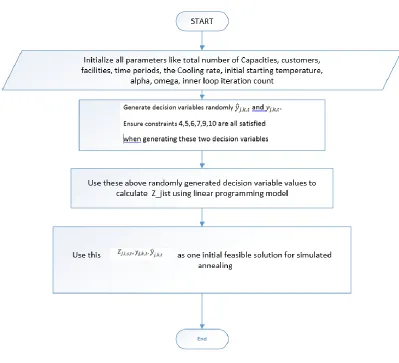
5.4 Initial Solution Generation ... 55
5.5 Neighborhood Generation Function ... 57
5.6 Explanation ... 64
5.7. SA Test Case ... 70
5.7.1 Test Case 1 ... 70
5.7.2 Test Case 2 ... 71
5.7.3 Test Case 3 ... 72
5.7.4 Test Case 4 ... 73
5.8 Discussion ... 74
5.9 Result of Simulated Annealing ... 75
6 Conclusion and Future Work ... 75
Bibliography ... 78
Appendix ... 83
1. Xpress code for Mathematical Modelling ... 83
2. Flowcharts ... 90
ix
List of Figures
FIGURE 1: RESEARCH APPROACH ... 7
FIGURE 2CROSS BORDER SUPPLY CHAIN USA–CANADA ... 24
FIGURE 3 CROSS BORDER SUPPLY CHAIN ... 41
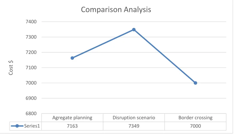
FIGURE 4 COMPARISON ANALYSIS ... 50
FIGURE 5SIMULATED ANNEALING GRAPHICAL REPRESENTATION ... 52
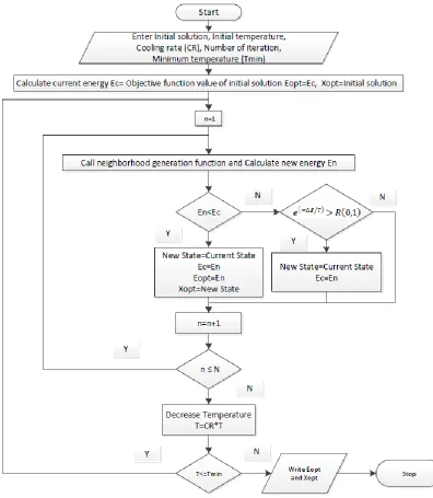
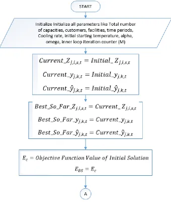
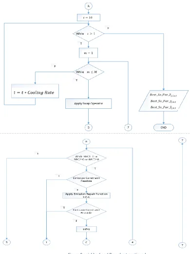
FIGURE 6SAALGORITHM FLOWCHART ... 54
FIGURE 7INITIAL SOLUTION ALGORITHM FLOWCHART ... 56
FIGURE 8NEIGHBORHOOD ALGORITHM FLOW CHART ... 59
FIGURE 9 FLOW CHART CONTINUED ... 60
FIGURE 10 FLOW CHART CONTINUED ... 61
FIGURE 11 FLOW CHART CONTINUED ... 62
FIGURE 12SWAP OPERATOR FLOW CHART ... 90
FIGURE 13SWAP OPERATOR FLOW CHART CONTINUED ... 91
FIGURE 14SWAP OPERATOR FLOW CHART CONTINUED ... 92
FIGURE 15SWAP OPERATOR FLOW CHART CONTINUED ... 93
FIGURE 16CONSTRAINT 5 FLOW CHART ... 94
FIGURE 17DECISION VARIABLE GENERATION FLOW CHART ... 95
FIGURE 18DEMAND REPAIR FUNCTION FLOW CHART ... 96
FIGURE 19DEMAND REPAIR FUNCTION FLOW CHART CONTINUED ... 97
FIGURE 20 EMISSION REPAIR FUNCTION FLOW CHART ... 98
FIGURE 21 EMISSION REPAIR FUNCTION FLOW CHART ... 99
FIGURE 22EXCESS REPAIR FUNCTION FLOW CHART ... 100
FIGURE 23EXCESS REPAIR FUNCTION FLOW CHART ... 101
FIGURE 24CONSTRAINT 4 FLOW CHART ... 102
FIGURE 25MERGE OPERATOR FLOW CHART ... 103
FIGURE 26MERGE OPERATOR FLOW CHART CONTINUED ... 104
FIGURE 27PRODUCTION REPAIR FUNCTION FLOW CHART ... 105
FIGURE 28RHS REPAIR FUNCTION FLOW CHART ... 107
x
List of Tables
TABLE 1DELAY TIMES AT BRIDGES ... 3
TABLE 2 Y_(J,K,T) VALUES_NO BORDER ... 36
TABLE 3 Z_(J,I,S,T)VALUES_TIME1_NO BORDER ... 37
TABLE 4:ZJIST VALUES_TIME2_NO BORDER ... 37
TABLE 5:AGGREGATE PLANNING ... 38
TABLE 6:SUPPLIER DEFAULT CAPACITIES ... 39
TABLE 7:CUSTOMER DEMAND ... 40
TABLE 8: AGGREGATE PLANNING ... 40
TABLE 9: 𝒚𝒋, 𝒌, 𝒕DECISION VARIABLE ... 42
TABLE 10:𝑍𝑗, 𝑖, 𝑠, 𝑡 DECISION VARIABLE TIME PERIOD 1... 42
TABLE 11: 𝑍𝑗, 𝑖, 𝑠, 𝑡 DECISION VARIABLE TIME PERIOD 2 ... 42
TABLE 12: 𝑍𝑗, 𝑖, 𝑠, 𝑡VALUES_TIME1_SCENARIO CASE ... 45
TABLE 13:𝒁𝒋, 𝒊, 𝒔, 𝒕VALUES_TIME2_SCENARIO CASE ... 46
TABLE 14:𝒁𝒋, 𝒊, 𝒔, 𝒕 VALUES_TIME1_DEMAND RATE ... 48
TABLE 15: 𝒁𝒋, 𝒊, 𝒔, 𝒕VALUES_TIME2_DEMAND RATE ... 49
TABLE 16: 𝑦𝑗, 𝑘, 𝑡 VALUES_DEMAND RATE ... 49
TABLE 17 Y_(J,K,T) VALUES IN CONSTRAINT 5 ... 64
TABLE 18 Y_(J,K,T) VALUES IN CONSTRAINT 5 ... 64
TABLE 19 Y ̂_(J,K,T) VALUES AS PER CONSTRAINT 4 ... 65
TABLE 20 Y ̂_(J,K,T) VALUES AS PER CONSTRAINT 4 ... 65
TABLE 21 Y_(J,K,T) VALUES ... 65
TABLE 22 Y_(J,K,T) VALUES ... 65
TABLE 23 Y_(J,K,T) AND Y ̂_(J,K,T) VALUES ... 67
TABLE 24 Y_(J,K,T) AND Y ̂_(J,K,T) VALUES ... 67
TABLE 25SATEST CASE 1 SIZE ... 70
TABLE 26SATEST CASE 1 RESULTS ... 70
TABLE 27SATEST CASE 2 SIZE ... 71
TABLE 28SATEST CASE 2 RESULTS ... 71
TABLE 29SATEST CASE 3 SIZE ... 72
TABLE 30SATEST CASE 3 RESULTS ... 72
TABLE 31SATEST CASE 4 SIZE ... 73
TABLE 32SATEST CASE 4 RESULTS ... 73
xi
Abbreviations
ILP: Integer Linear Programming
MILP: Mixed Integer Linear Programming
SCND: Supply Chain Network Design
MFLAP: Multiple Facility Location Allocation Problem
SCM: Supply Chain Management
SA: Simulated Annealing
OR: Operation Research
FLAP: Facility Location Allocation Problem
GHG: Greenhouse Gas Emissions
CUSFTA: Canada-U.S. Free Trade Agreement
NAFTA: North American Free Trade Agreement
VRP: Vehicle Routing Problem
FMS: Flexible Manufacturing System
1
1
Introduction
1.1
Brief Introduction
In supply chain management (SCM), three planning levels are usually distinguished
depending on the time horizon. These three levels are strategic, tactical and operational. Strategic
level deals with decisions regarding number of facilities, capacity of each facility and the flow of
material through the logistics network. Facility location-allocation comes under strategic planning
and has been a well-established research area within Operations Research (OR). A facility location
allocation problem (FLAP) involves mapping a set of customers to a set of facilities that serve
customer demands. Constructing a mathematical linear programming model and a Meta-heuristic
algorithm is an efficient approach to optimize supply chain cost. Optimization results allow us to
decide quantity of goods to be transported from each facility to its respective customers.
Owing to the billion dollar trade between the USA-Canada the supply chain costs are growing.
Trade takes place via cross borders. These borders have disruptions. This problem is incurring high
costs to Canadian as well as US manufacturers. To represent this real life problem, an Integer
Linear Programming (ILP) mathematical model is formulated. This model incorporates several
parameters which would optimize the overall supply chain cost.Capacitated, single commodity,
and multiple time period (dynamic), multi-facility location allocation problem is more precise
description of the problem under consideration. Canada is a part of “The Kyoto protocol”, a United
Nations Framework Convention on Climate Change. Canada has declared to abide by global effort
to reduce greenhouse gas emissions (GHG) emissions. Due to this, Canadian government is
encouraging research to reduce (GHG) emissions. Math model includes an important constraint
which allows us to optimize production costs by keeping the Carbon di-oxide [𝐶𝑂2] emission levels
within specified limits. With increasing number of manufacturing facilities and customers over the
planning horizon, size of the problem increases. Integer Linear Programming (ILP) mathematical
model is in-capable to find solution in limited time and is computationally expensive. To solve
2
1.2
Statistical Background
Since the passage of the Canada-U.S. Free Trade Agreement (CUSFTA) in 1987 and North
American Free Trade Agreement (NAFTA), the U.S. and Canada have witnessed explosive
growth in trade. Following information obtained from Wikipedia, 2015 explains few details
about (CUSFTA):
1. Eliminate barriers to trade in goods and services.
2. Significantly liberalize conditions for investment within free-trade area and facilitate
conditions of fair competition.
3. Establish effective procedures for the joint administration of the Agreement and resolution
of disputes.
4. Lay the foundation for further bilateral and multilateral cooperation to expand and enhance
the benefits of the Agreement.
According to www.naftanow.org, 2013 following are a few details about
(NAFTA)
1. It has helped to stimulate economic growth and create higher-paying jobs across North
America.
2. It has paved the way for greater market competition and enhanced choice and purchasing
power for North American consumers, families, farmers, and businesses.
3. In 2008, Canada and the United States inward foreign direct investment stocks from NAFTA
partner countries reached US$469.8 billion.
4. North American employment levels have climbed nearly 23% since 1993, representing a net
gain of 39.7 million jobs.
5. The U.S. exports span more than 230 destinations, with Canada and Mexico accounting for
more than one-third of the total.
6. If we look at the latest figures at the Canadian side of trade statistics, in the first quarter of
the year 2015 a total of 89,321.2 million $ worth merchandise was imported from USA alone
and 95,536.9 million $ worth merchandise was exported to USA (www5.statcan.gc.ca,
statistics Canada, 2015).
7. Looking at the USA side of trade statistics, in 2013, US goods exports to Canada totaled $300
billion up by 77% from 2003 and goods imports totaled $332 billion. (Office of the United
3
8. Taking a look at the modes of transportation used for the supply chain, trucks carry
three-fifths of U.S.-NAFTA trade and are the most heavily utilized mode for moving goods.
9. Trucks carried 59.9 percent of U.S.-NAFTA trade in May 2014, accounting for $31.8 billion of
exports and $30.4 billion of imports.
10. In the year May 2013 to May 2014 trucks carried 53.9 percent of the $57.7 billion of freight
to and from Canada.
Considering above figures it can be concluded that huge amount of trade takes place between
USA-Canada. Growing trade increases the complexities in supply chain and hence there is
great need to design highly efficient supply chain network.
Border delays are generally the first costs cited in most border discussions. Not necessarily
because they are the most important costs, but because they are the most visible
manifestation of the thickened Canada-US border Anderson (2012). Following table will
illustrate and example to show delays (in minutes) at the Ontario-US bridges.
Table 1 Delay times at bridges
BRIDGE
STATISTICS AMBASSADOR BLUE WATER PEACE LEWISTON-QUEENSTON
MEAN 11.3 13.8 13.2 10.8
MEDIAN 7.6 7.5 7.9 5.2
STD .DEV 9.8 18.3 24.6 14.2
MIN 0.8 1 1.1 1
MAX 238.4 288.6 732.1 217.5
4
1.3
Motivation
In recent years, a considerable importance is given to the border security problems. The US
has initiated a need to "secure" the northern border. Border crossing processes and procedures
have received strict attention since 9/11. According to Taylor et al. (2004) causes of border delays
and their impacts have been grouped into infrastructure and institutional categories. Highly
scrutinized clearance procedures at the USA-Canada border is increasing in-transit inventory
holding costs for most manufacturers and suppliers. Further, there is uncertainty in border
clearances. Also, there is an uncertainty in time required for crossing USA-Canada border. This
has a worst financial impacts on overall supply chain. More specifically, delay- and uncertainty
related costs were estimated to total US$4.01 billion Taylor et al. (2004) These costs represent
1.05 percent of total merchandise trade, or 1.58 percent of truck-borne. According to Wigle and
Randall (2009) it is estimated that border delays could cost truckers, on an average, about 32
minutes per shipment. This incurs C$290 million per year for Canadian exporters. These additional
costs incurred is loss of business, and definitely imply a need for optimization.
Primary causes of delay at USA-Canada border are as follows-:
1. Infrastructure: Number of booths at border crossing in proportion to number of vehicles
crossing the border.
2. Human resources: According to the USA homeland security website, amount of staff recruited
at USA-Canada border for processing merchandise is not sufficient enough.
Both of these issues are non-technical or related to government administrative policies. Hence,
those are beyond our scope of discussion. However, monetary losses associated with the
USA-Canada border delays needs to be addressed. To optimize these costs, we have considered to
5
Following figure gives few causes at the USA-Canada border (Source: TAYLOR et al. (2004)
1. Number of Toll booths
2. Exit check points at the US side
3. Road bed capacity
4. Inspection plazas
5. Processing of line release paper work prior to arrival of carriers not occurring
6. Amount of Staff levels
7. Institutional /Management issues
8. Processing time per vehicle
9. Hours of operation
10. Secondary inspection yards size and availability of parking
6
1.4
Research Objectives
The primary goal of this thesis is to optimize the overall cost incurred in the USA-Canada
cross border supply chain network. Approach to achieve these objectives is to develop ILP
mathematical model that will allow deciding the optimal quantities of goods to be produced and
shipped by each facility each year. Furthermore, since the model developed is capacitated
dynamic facility location allocation, the goal also includes determining the production capacities
to be installed at each facility each time period. In a multi-period problem, the customer demand
is dynamic and changes over the period of time. Because of customer demand change, the
developed model allows dismantling of installed production capacities in order to optimize the
production quantity for each facility. Cost component in the developed ILP includes costs
associated in construction and dismantling of capacities, domestic and cross border cost of
transportation. For determining the optimized production quantities for each facility these supply
chain costs associated with corresponding parameters are considered. Additional constraints
include limiting the production of each facility such that carbon-di-oxide emissions are maintained
within international permissible values.
1.5
Problem and Thesis Statement
“Highly scrutinized clearance procedures at the USA-Canada border is increasing in-transit
inventory holding costs resulting in major monetary losses for Canadian exporters. Primarily, to
reduce these monetary losses while keeping
co
2emission level within permissible values, webelieve that an optimized design of cross border supply chain network is necessary. Designing an
Integer Linear Programming model and constructing a meta-heuristic would be an efficient way
7
1.6
Research Approach
An extensive literature review is done to identify which parameters affect supply
chain network design. Based on all available parameters, decision variables are chosen.
The key decision variables are identified and finalized. These decision variables are
discussed in chapter 3 of this thesis. Integer linear programming model is developed. As
the size of the problem goes on increasing, it was found that ILP is incapable to give results
in less time and is computationally expensive. For example, if number of facilities and
customers is high, problem being NP hard, grows exponentially and commercially
available optimizing software is unable to reach to optimal solution in finite time. Hence,
we develop a simulated annealing based meta-heuristic to obtain near optimal solution.
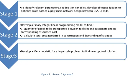
Figure 1 : Research Approach
Stage 1
•To identify relevant parameters, set decision variables, develop objective fuction to optimize cross border supply chain network design between USA-Canada.
Stage 2
•Develop a Binary Integer linear programming model to find-:
•1. Quantity of goods to be transported between facilities and customers and its corresponding associated cost
•2. Calculate total cost associated in construction and dismantling of facilities
Stage3
8
2
Literature review
Supply chain could be defined as a link between various entities of any organization. Supply
chain management (SCM) is a strategy through which such integration can be achieved. Supply
chain network design (SCND) is a complex undertaking. It involves determining which facilities to
include in the supply chain network (e.g., plants, warehouses), their size and location (Correia et
al. 2013). Supply chain also establishes the transportation links among the members of the supply
chain and setting the flow of materials through them. Supply chain network design problems
could be classified under two main categories:
1. Multiple Facility Location Problem (MFLP)
2. Multiple Facility Location Allocation Problem (MFLAP)
In multiple facility location problem the aim is to find optimal location for each facility.
Examples include P-median type of problems, capacitated and un-capacitated facility location
problem. On the other hand, multiple facility location allocation problem aims at establishing
optimum location to a facility. Further, it wishes to determine optimum amount of goods to be
transported from a facility to its assigned customer.
Multiple Facility Location Allocation problems are NP hard (Y. Hinojosa et al., 2000). This class
of problems address the objective of assigning best location for the facilities, decide which
facilities would serve which customer and what should be the optimal quantity to be transported.
This gives optimum cost of transportation involved. While assigning facilities to locations new
facilities can be set up over the planning horizon. This problem is capacitated, single commodity,
multiple facility, and multiple time period location allocation problem. Also,this problem address
changing customer demand over the planning horizon. Dynamic location allocation problem aims
to answer three important questions. Firstly, which are the best places to locate the available
facilities. Secondly, what is the best capacity to assign to the generic logistic facility. Thirdly, at
which period of time, what should be the amount of production capacity. Hence, according to
Gebennini (2008) “Capacitated, single commodity, multiple facility, and multiple time period
(dynamic) facility location allocation problem” will be a complete definition for this class of
9
2.1
Supply Chain Network Design Literature Review
Isabel Correia , Teresa Melo and Francisco Saldanha-da-Gama (2013) compare classical
performance measures for a multi-period, two-echelon supply chain network design problem
with sizing decisions. They consider a problem of structural decisions to be made over a
multi-period planning horizon as follows:
(i) Selection of new facilities from a given set of candidates
(ii) Facility capacity management through the installation of storage areas for each product family
at each open location
(iii) Investment of the available budget for facility location and capacity.
Further decisions concern the quantities of products to be shipped from the upper level facilities
to the intermediate level facilities (two echelon), and from the latter to customer zones.
Comparison of cost optimization and profit maximization models is done using MILP. However,
the linear relaxation bound of the MILP formulation proved to be rather weak in most of the test
instances. In particular, solution quality seems to deteriorate as the number of time periods
increases.
Ali Amiri (2006) addresses the problem of designing a distribution network for a supply chain
system. The goal is to determine the optimum number of plants, optimum locations and optimum
assignment of capacities to plants and warehouses. Customer demand is to be satisfied at a
minimum total costs of the distribution network. Here, use of multiple level of capacities is done.
The author formulates a mixed integer linear programming.
A linear relaxation-based heuristic approach for logistics network design is presented by
Thanh et al. (2010). The authors design a multi-period, multi-echelon, multi-commodity logistics
network with deterministic demands. This consists of making strategic and tactical decisions like
opening, closing or expanding facilities, selecting suppliers, selecting capacity planning and finally
defining the product flow. Planning horizon is 5 years. Heuristic approach of successive linear
relaxation of the original mixed integer linear problem (MILP) is formulated in this paper. The
main benefit of this approach is that it provides a feasible solution of good quality within an
affordable computation time. Major drawback is that customer demand is deterministic and
certain.
Capacitated dynamic location problems with opening, closure and reopening of facilities is
10
the possibility of reconfiguring one location more than once during the planning horizon. Primal–
dual heuristic is developed
Capacity based supply chain network design considering demand uncertainty and using
two-stage stochastic programming is different aspect studied by Mishra et al. (2013). Their model also
considers inventory carrying cost, opportunity cost in addition to investment cost, processing
cost, and transportation cost. The objective of the proposed model is two fold. Firstly,to evaluate
optimal locations of echelons and secondly, to determine the quantities flow between them. The
objective is to minimize overall cost. However, the model has several assumptions:
1. Probabilities of future economies/market demand is selected at random.
2. Their model does not consider plant capacities as discrete values. Plant capacities are in range.
Results of their paper show that few plants have excess capacities assigned ,which contradicts the
optimum results.
Multi-level supply chain network design with routing has been studied by Lee et al. (2010).
The purpose of their study is to determine the optimal location for facilities, allocation of facilities
to customers, and routing for transporting goods. The objective is to design a minimum cost
supply chain network. The authors develop a mixed integer programming model for SCND routing.
Further, their own heuristic algorithm is developed. The authors conclude that heuristic results
are better than MILP results. However, potential drawback in their paper is that there is a
maximum capacity restriction.
Optimization models for the dynamic facility location and allocation problem has been
studied by Gebennini et al. (2008). The aim of their study is to develop and apply innovative mixed
integer programming optimization models to design and manage dynamic (i.e. multi-period)
multi-stage and multi-commodity location allocation problems (LAP). They formulate a mixed
integer linear programming model. They have applied the model to real life test case. The best
solution guarantees a cost reduction of approximately 900000/year. They claim that the proposed
model gives solution in less time and do not need to design ad-hoc solving algorithms. However,
stochastic demand is not considered in their model. Also, none of the existing facilities are
dismantled and constructed again.
A multi period two-echelon multi commodity capacitated plant location problem is studied
11
customer demands and transportation costs change over the time periods. They do not consider
inventory holding decisions. Goal of their research is to minimize the total cost for meeting
customer demands. The customer demand varies for different products over the period of time.
Firstly, they develop MILP and then a heuristic. However, from the results it can be confirmed that
the computation time is very high for MILP model. Also, once a facility is dismantled it cannot be
constructed again. Infeasible solution is obtained when Lagrangean relaxation is used.
An exact method for a two-echelon, single-source, capacitated facility location problem is
studied by Tragantalerngsak et al. (2000). In this research paper, the number and location of
facilities in two echelons along with the allocation of customers to the second-echelon facilities is
to be determined simultaneously. They develop a branch and bound algorithm for a two echelon
single source capacitated facility location problem based on the most efficient Lagrangian
heuristic. Lagrangian relaxation approach produces significantly smaller B&B trees and consumes
much less computing time. However, their approach has a shortcoming in which each customer
is serviced by only one facility in the second echelon.
An algorithm for the capacitated, multi-commodity, multi-period facility location problem
has been studied Cem Canel et al. (2001). They develop a MILP and then a heuristic algorithm
using Bender's decomposition approach. They include a constraints such that the total capacity
of open facilities must exceed the total demand of all customers in each period. Drawbacks
include that no direct shipment is allowed from facility to customer.
Melkote and Daskin (2001) study capacitated facility location/network design problem. In
this problem, authors have combined both facility location and network design which are usually
different aspects of supply chain. Facilities have capacity constraint. They develop MILP and LP
relaxation using branch and bound. However, they have assumed that customer demand and
facility construction cost is normally distributed. Minimum capacity of each facility is assumed
equal. They conclude that both link costs and transport costs may actually decrease when capacity
constraint is enabled.
A heuristic for the ILP problem like single source capacitated facility location problem has
been studied by Guastaroba and Speranza (2014). In their paper, each customer is assigned to a
12
all the customers. Kernel search heuristic framework is applied to ILP. They conclude that large
size problem can be solved in less time to optimality. However, their problem is not multi-period.
A tabu search heuristic procedure for the capacitated facility location problem is given by
Minghe (2012). Three phases like criterion altering, solution reconciling and path relinking are
used for the intensification process in the tabu search procedure. The method of Lagrangean
relaxation with improved sub-gradient scheme (LRISS) developed by Lorena and Senne (1999) is
used as a benchmark to measure the effectiveness and efficiency of the tabu search procedure.
They assume that, their heuristic starts the solution process of the current iteration from the
optimal solution of the previous iteration.
Arabani and Farahani (2012) present the facility location dynamics overview. They present
latest classification of facility location and allocation problems. They also present the
mathematical formulations used for each kind of facility location problem.
Some research papers consider inventory optimization. An integrated production
distribution model for the dynamic location and allocation problem is considered by authors like
Manzini et al. (2009). Additionally, safety stock optimization is achieved in their results. Cost based
optimization of supply chain is achieved by integrating strategic, tactical, and operational
decision-making. These decisions are related to the design, management, and control of activities.
The cost-based and mixed-integer programming model presented has been developed to support
management in making decisions like deciding number of facilities (e.g. warehousing systems,
distribution centers), choice of locations and assignment of customer demand to facilities. Their
paper also incorporates tactical decisions regarding inventory control, production rates, and
service-level. Nonlinear objective function is linearized for MILP model. Customer demand is
assumed as normal distribution. A major assumption is that all distances are considered as
Euclidian distances.
Un-capacitated facility location problem with demand-dependent setup and service costs is
considered by Averbakh et al. (2007). The paper gives an insight of some mathematical models
which have used un-capacitated facilities. One of the objectives is to choose locations for facilities
and balance prices. Other o-bjective is to minimize the expenses of the service company. These
expenses include the sum of the total setup costs and total transportation costs. Polynomial time
13
Optimal production allocation and supply chain distribution network design is considered by
Tsiakisa and Papageorgiou (2008). The objective of their work is to determine the optimal
configuration of a production and distribution network. They include operational and financial
constraints in their mathematical model. Their work considers the optimal design and operation
of multi-product, multi-echelon global production and distribution networks. The network
consists of finding number of existing multi-product manufacturing sites at fixed locations, a
number of distribution centers, and finally a number of customer zones at fixed locations using
MILP. The best thing about the model is that it aims to assist senior operations management to
take decisions regarding production allocation, production capacity per site, purchase of raw
materials and network configuration. These decisions take into account financial aspects
(exchange rates, duties, etc.) and costs. However, some decisions are already assumed. Decisions
such as customer allocation to distribution centers are already defined. Other drawback is that
each plant can manufacture a maximum of three products.
A dynamic model for facility location in the design of complex supply chain is presented by
Thanha et al. (2008). Their research paper considers multi-period, multi-commodity multi-facility
location problem. In their mathematical model all customer demands are deterministic. This
research paper aims to help strategic and tactical decision making like opening-closing or
enlargement of facilities, supplier selection and determine material flow along the supply chain.
However, they have some assumption. Firstly, status of a facility changes only once during the
entire planning period. Secondly, closed facilities cannot be reopened while new facilities will
remain active until the end of the planning horizon.
Solving complex multi-period location models using simulated annealing is studied by
Antunes & Peeter in 2001 .In this paper multi-period location problems raised by school network
planning in Portugal is studied. The problem is formulated as mixed-integer linear optimization
model. The model allows for facility closure or size reduction. Also, facility opening and size
expansion can be done. These expansions are done with sizes possibly limited to a set of
pre-defined standards. The study described in this paper shows that simulated annealing may be a
good resort when solving complex mid-size multi-period location problems. However, the
drawbacks of this paper is that computational time is very high. Also simulated annealing
14
solution. This decided percentage is problem specific and hence cannot be applied to generic
problem.
Solving location allocation problem using rectilinear distances using simulated annealing
heuristic algorithm is studied by Chih-Ming Liu et.al (1994). They deal with finding total number
of new facilities to be opened, allocation of facilities to customers and the location of the facilities
in order to optimize the entire supply chain. For perturbation they are randomly choosing a facility
which has not been chosen before and allocating a customer to it. They then calculate the
objective function cost and compare it with previous iteration. The authors generate initial
solution randomly. They compare their solution with two other heuristics and conclude that
simulated annealing heuristic has better solution. Their problem differs from the one considered
in this thesis because they are considering rectilinear distances between facilities.
Bi-level simulated annealing algorithm for facility location problem is studied by Ren Peng
et.al (2008). Authors have invented Bi-level simulated annealing logics which they call as inner
layer simulated annealing logic and outer layer simulated annealing logic. According to which they
have decision variables which decide whether to open a facility at location and allocation of the
facility to the customer. The outer layer logic decides at which locations facilities should be
opened and then it uses add, exchange or remove operator to decide at which locations facilities
have to be constructed. The inner layer logic is for optimizing demand allocation. It explains that
if a facility is initially allocated to for a customer then using swap operator, the authors generate
new combination and calculate objective costs. They conclude that solution is near global
optimum and their computation time is also less.
In a private communication, M.F. Baki (2016) mentions the following:
“G. Pandher initiates a research “location problem with border disruption risk” through a grant
from the Cross-Border Institute (CBI) at the University of Windsor in 2013. E. Selvarajah
collaborates on this research for some time in the beginning. H. Rajput works on this project till
November, 2013. In a meeting on December 2, 2013, G. Pandher presented an unpublished note
(Author Unknown, 2013) developed through his CBI-grant. The note identifies multiple disruption
scenarios that occur on a supply chain network and that’s relevant for the facility location
decisions. The note develops a single-source binary-integer-program (BIP) facility location model
15
restriction on the maximum number of facilities. The model uses a two-index decision variable 𝑥𝑗𝑖
which is 1, if customer 𝑖 is served by facility 𝑗 and which is 0, otherwise. The model also uses a
decision variable 𝑦𝑗 which 1, if a facility 𝑗 is set-up and which is 0, otherwise. The model puts a
restriction that every customer must purchase all its demand from a single facility and another
restriction on the maximum number of facilities.
M.F Baki presents a model on December 9, 2013 and four more models on January 10, 2014. The
models are labelled in an increasing order of complexity and difficulty. Models 1 and 2 are
single-sourcing models with 3-index decision variables 𝑥𝑗𝑖𝑠 and Models 3, 4, 5 are capacitated models.
Model 1 and all the other models ensure that the sourcing decisions may be different in different
scenario, although the facility location decision is the same over all scenarios. Model 1 minimizes
the sum of the facility setup cost and the expected production and transportation costs. Model 2
partitions the set of supply chain transportation links into domestic and cross-border subsets 𝐸1
and 𝐸2. The expected costs at the domestic links are affected by the probability of scenario 𝑝𝑠
only, but the expected costs at the cross-border links are affected by 𝑝𝑠 and 𝑒𝑠, where 𝑒𝑠
represents the increase in the cost of scenario 𝑠. Model 3 introduces fixed capacity of facilities,
capacity additions and dismantling. Model 4 gives a different sourcing decision in a different time
period. Model 5 gives a different sourcing decision for a different product. Out of these 5 models,
Model 2 is used without modification in (Pandher and Baki, 2015) and Model 4 is extended
significantly in this thesis.”
Pandher and Baki (2015) developed expected cost of disruption which is a function of the length
and frequency of disruption. Similarly they formulate a novel function called “critical cost of
disruption”. If expected cost of disruption exceeds the critical cost of disruption, the optimal
location decision changes from one supply facility on one side of the border to two supply facilities
on two sides of the border. To describe their linear programming model, they have given a small
example in which they conduct break even analysis for deciding the construction of facilities at
two possible locations. They prove that if the expected cost of disruption is greater than critical
cost of disruption the optimal location decision changes. Further, they discuss the effect of
increase in cost due to increase in length and frequency of disruption. Additionally, they study the
effect of population / size of demand by comparing the critical cost function of two demand
16
Research paper has also been studied. According to ReVelle and Swain (1970) research in which
the authors have introduced a p-median problem.
Objective function is to minimize
∑ ∑ 𝑝𝑖𝑑𝑖,𝑗𝑦𝑗,𝑖
𝑖∈𝐼 𝑗∈𝐽
Constraints:
∑𝑗∈𝐽𝑦𝑗,𝑖= 1 ∀ 𝑖 ∈ 𝐼 (1)
𝑦𝑗,𝑖≤ 𝑥𝑗 ∀ 𝑖 ∈ 𝐼 , j ∈ 𝐽 (2)
∑𝑗∈𝐽𝑥𝑗= 𝑝 (3)
𝑑𝑖,𝑗 is distance and 𝑝𝑖 is the customer demand. Constraint (1) ensures that customer demand is
satisfied completely by a single facility. Constraint (2) tells that if a facility is not constructed then
it cannot supply to customer. Constraint (3) total number of built DCs should be equal to specified
number.
Hoda A. ElMaraghy (2006) writes a paper of Fexible and reconfigurable manufacturing systems
paradigms. In this paper she mentions that RMS promises customized flexibility on demand in a
short time, while Flexible Manufacturing System (FMS) provides generalized flexibility designed
for the anticipated variations and built-in a priori. The key feature of RMS is that, unlike FMS, its
capacity and functionality are not fixed (Mehrabi et al., 2000). ElMaraghy further mentions the
key definitions of RMS and FMS. As per the author, RMS is designed at the outset for a possible
rapid change in structure, as well as in hardware and software components, in order to quickly
adjust production capacity and functionality within a part family. An FMS is a system whose
machines are able to perform operations on a random sequence of parts of different types with
little or no time or other expenditure for changeover.
“Mechanics of Change: A framework to reconfigure manufacturing systems” by Azab et al. (2013)
describes manufacturing system reconfiguration as a controller, which minimizes the deviation
17
Their aim is to design adjustable reconfigurable solutions to minimize the cost while aligning the
change requirements with the system performance measure. For that they introduce a control
loop approach for change synchronization. The author also gives detail explanation on system
level and machine level reconfiguration methodologies.
“A Reconfigurable Manufacturing System (RMS) is one designed at the outset for rapid change in
structure, as well as in hardware and software components, in order to quickly adjust production
capacity and functionality within a part family in response to sudden changes in market or in
regulatory requirements” Koren et al.(1999) The concept of a RMS designed specifically for
scalability was first introduced by Spicer et al.(2002). This concept, called scalable-RMS, provides
the option of adding and removing multiple identical modules.
“A reconfigurable manufacturing system (RMS) that is designed specifically to adapt to changes
in production capacity, through system reconfiguration, is called a scalable-reconfigurable
manufacturing system” Spicer and Carlo (2007). This definition allows us to derive a relation that
a manufacturing facility can be reconfigurable and the system installed in it can be made scalable.
Hence, we can say that scalability is an attribute of reconfigurable manufacturing facility.
“With reconfigurable manufacturing systems on the other hand, capacity scalability addresses
the reduction of capacity besides the expansion.” Deif and ElMaraghy (2006).
Wilhelm et al. (2013) discuss the computational comparison of two formulations for dynamic
supply chain reconfiguration with capacity expansion and contraction. Their problem is to
prescribe the location and capacity of each facility, select links used for transportation, and plan
material flows through the supply chain, including production, inventory, backorder, and out
sourcing levels. Research objectives of this paper area traditional formulation and a
network-based model of the problem. Their paper clearly defines concept of a “reconfigurable
manufacturing facility” in terms of a facility location allocation problem. This paper is used to
benchmark and develop the title of our thesis.
Facility Location Problem for Reconfigurable Manufacturing System (RMS) with Changing
Multi-Period Demand is the title of the research paper written by Jeong and Seo (2008). Short product
life-cycles and varied customer demands result in use of reconfigurable manufacturing systems
18
operation plan for Reconfigurable Manufacturing System, and material flow quantity between
facilities in a supply chain network. In their paper, they focus on FLP in which RMS, Distribution
centers and retailer are facilities of SCN. Reconfigurable Manufacturing System produces the
products, Distribution centers distributes the products from RMS to retailers, and retailer meets
customer demands. Hence the manufacturing facility having a Reconfigurable Manufacturing
System (RMS) is termed as a reconfigurable facility. This paper is thus referred in for defining the
relation between RMS and how a facility can be considered as a reconfigurable.
2.2 Emission Literature Review
When an organization becomes multinational it acquires customers across various countries.
To supply its customers, it establishes global supply chain network. With the growing demand
across the globe, size of supply chain also increases exponentially. With every route added in
supply chain there is an increase in mode of transportation which is inevitable. Due to this ever
increasing number of vehicles there is a tremendous increase in the carbon dioxide emission.
These vehicles burn fossil fuels. Thus, some leading companies are now proactively implementing
“green” initiatives. For example, the largest furniture manufacturer, IEKA, built a train
transportation network with an emphasis on the “greenness” of train operations. HP, IBM, and
GE are all taking “green” as an important merit in their enterprise's value systems in order to
maintain good public image. They are designing greener products by adopting new energy saving
technology Wang et al. (2010). The temperature of the earth has increased by 0.8 degrees Celsius
between 1900 and 2005. Freight transport in the United Kingdom is responsible for 21% of the
carbon-di-oxide emissions from the transport sector, amounting to 33.7 million tons or 6% of the
carbon-di-oxide emissions in the country. Out of the total, road transport accounts for a
proportion of 92% (McKinnon, 2007). Similar figures apply to the United States, where the
percentage of total GHG emissions due to transportation rose from 24.9% to 27.3% between 1990
and 2005. Road transport alone accounts for 78% of the emission produced by all transportation
modes (Ohnishi, 2008). There are number of active carbon markets for GHG emissions such as the
European Union Emission Trading Scheme (EU ETS) in Europe. This is the largest multi-national
GHG emissions trading scheme in the world. Few other carbon trading markets include New
19
United States and more recently the Montreal Climate Exchange in Canada. According to
Chaabane et al. (2010) GHG emissions are calculated based on emission factors and are converted
to carbon dioxide equivalent quantity. Diabat and Simchi-Levi (2009) explain details about kyoto
protocol. Kyoto protocol, a part of the United Nations Framework Convention on Climate Change,
was negotiated as a part of global effort to reduce GHG emissions. The protocol establishes legally
binding commitments on all member nations to reduce their GHG emissions. The working of Kyoto
protocol is as follows:
1. Every member country government establishes a limit on total emission in fixed duration of
time.
2. To achieve its emission targets government sets carbon emission restrictions on each industry
and encourages them to use green technologies so as to reduce pollution.
3. Every industry receives fixed amount of carbon credits at beginning of planning horizon. Each
carbon credit permits 1 Ton carbon dioxide emission in the atmosphere.
4. Once the company uses its credits it can buy more credits at some price from the government
or from the companies which have excess credits left. This is called carbon trading. By this way
every company or organization tends to save more credits and eventually money by turning
towards green operational technologies.
5. Additionally, if the company is able to achieve its emission targets, it gets economic incentives
from governments.
Green logistics has recently received increasing and close attention from governments and
business organizations. The importance of green logistics is motivated by the fact that current
production and distribution logistics strategies are not sustainable in the long term. Thus
environmental, ecological and social effects are taken into consideration when designing logistics
policies. Additionally, conventional economic costs are also considered. The environmentally
sensitive logistic policy requires changing the transportation scheme. Such policy will have fewer
negative impacts on the environment and the ecology. This is because transportation accounts
for the major part of logistics. There is a wide variety of problems concerning green
transportation, such as the promotion of alternative fuels, next-generation electronic vehicles,
green intelligent transportation systems, and other eco-friendly infrastructures. According to
Canhong Lin (2014) better utilization of vehicles and a cost effective vehicle routing solution
20
A multi-objective optimization model for green supply chain network design is studied by
Wang et al. (2010). They try to achieve trade-off between the total cost and the environment
influence. However, if the emission per facility is to be considered then they haven’t considered
demand uncertainty.
Routing is considered by Bektas and Laporte (2011). They study which route has to be
considered so as to optimize those not just for the travel distance, but also for the amount of
greenhouse emissions, fuel, travel times and their costs. Managerial insights shade light on
tradeoffs between various parameters such as vehicle load, speed and total cost, and offers
insight on economies of ‘environmental-friendly’ vehicle routing. This research paper’s
contributions include (i) Incorporation of fuel consumption and carbon-di-oxide emissions into
existing planning methods for vehicle routing (ii) Development of a new integer programming
formulation for the VRP. This novel mathematical model, in contrast to most of the existing
models, minimizes a total cost function which includes emission constraint. This cost function is
composed of labor, fuel and emission costs expressed as a function of load and speed.
Design of sustainable supply chains under the emission trading scheme is studied by
Chaabane et al. (2010). This paper introduces a mixed-integer linear programming based
framework for sustainable supply chain design. Their mathematical model considers life cycle
assessment (LCA) principles in addition to the traditional material balance constraints at each
node in the supply chain. It considers limit on carbon emission and determines the number of
carbon credits to be bought and sold.
Green supply chain network design to reduce carbon emissions is discussed by authors
Elhedhli and Merrick (2012). The relationship between carbon-di-oxide emissions and vehicle
weight is modeled using a concave function leading to a concave minimization problem.
Lagrangian relaxation is used to decompose the problem into a capacitated facility location
problem with single sourcing. This makes it a concave knapsack problem that can be solved.
Concave mixed integer programming model is tackled using Lagrangian relaxation.
Research paper written by Absi et al. (2013) explains lot sizing with carbon emission
constraints. This research paper deals with finding the carbon emission per product produced.
The authors consider periodic carbon emission constraint, rolling carbon emission constraint,
cumulative carbon emission constraint, and global carbon emission constraint.
Green supply chain network optimization and the trade-off between environmental and
21
emissions, costs of the supply chain contingent upon the production volume allocation and the
energy mix. The results, based on a case study in the German automotive industry, show that by
optimizing the energy mix, the carbon-di-oxide emissions of the supply chain can be reduced by
30% at almost zero variable cost increase.
The single-item green lot-sizing problem with fixed carbon emissions has been discussed by
Absi et al . (2015). The research paper efficiently explains how to calculate the amount of emission
per product. The problem deals with determining which node to be selected in each period such
that no carbon emission constraint is violated. Further, cost of satisfying all the demands on a
given time horizon is also minimized. MILP model is formulated.
The economic lot-sizing problem with an emission capacity constraint is studied by Helmrich
et al. (2015). Authors calculate the emission per unit production. They provide a Lagrangian
heuristic to provide a feasible solution. For costs and emissions values such that the zero inventory
property is satisfied, they give a pseudo-polynomial algorithm, which can also be used to identify
the complete set of Pareto optimal solutions of the bi-objective lot-sizing problem. Furthermore,
for such costs and emissions, they present a fully polynomial time approximation scheme (FPTAS).
They extend it to deal with general costs and emissions. Special attention is paid to an efficient
implementation. An improved rounding technique is used to reduce the posteriori gap. The same
technique is also used for combination of the FPTAS and heuristic lower bound. Extensive
computational tests show that the Lagrangian heuristic gives solutions that are very close to the
optimum.
Authors Xiaoli and Li (2010) research on the optimization of carbon emissions from
distribution centers and propose Genetic algorithm for solving large size problem. The concept
behind this research area is that emission is associated even with inventory. This paper proposes
a MILP model to decide optimum locations of distribution centers. This research paper aims to
minimize the carbon emissions of entire logistics system. Euclidean distance is considered
between facility and warehouse and demand points. However, they do not consider emission
22
2.3
Research Contribution
The primary objective of any SCND model has always been the identification of the network
configuration with the least total cost. According to Correia et al. (2013) facility location and
logistics costs (e.g., for production and distribution) are among the most frequent cost
components.
The contribution of this thesis in comparison to the existing literature is as follows:
1. Modelling, formulation and design of the USA-Canada cross border supply chain network itself
is a new emerging research area. FLAP have been studied before. However, its specific application
to USA-Canada cross border supply chain considering disruption has never been done before. In
this thesis we address FLAP specific to the USA-Canada cross border SCND.
2. Disruption scenario specific to customer demand and the probability of occurrence of
corresponding disruption scenarios have not been considered previously in any mixed integer
linear programming model.
3. In this thesis, a novel emission constraint has been introduced in supply chain network design
to limit the amount of Carbon-di-oxide emission below permissible limits per manufacturer per
year. Also, to the author’s knowledge a simulated annealing based metaheuristic for FLAP
23
3
Methodology
3.1
Problem Description
Mathematical model developed in this thesis consists of set of locations (V) and customers
(
U
) spread across the USA and Canada. Each location has a facility with default existing production capacity (𝐻
𝑘 ). This assigned capacity can be added / dismantled, from predefined set ofcapacities, based on changing customer demand over the planning horizon. Cost is incurred
whenever a capacity is added / dismantled to an existing capacity. Customer demand can be
satisfied by multiple facilities. In the developed model, customer demand parameter is
deterministic and changes with time. For each time period demand is fixed and supply should be
greater than or equal to demand.
Scenario can be described as a specific event or instance. For example: consider a disruption
scenario let’s say “Orange alert at Ambassador Bridge”. Assume that this scenario occurs. To
incorporate this scenario in our model we consider the probability of occurrence of this scenario
(Ps). The user can set probability of scenario as per measures. Model is developed in such a way
that a single time period contains multiple scenarios.
Customer demand is discrete but deterministic and changes with respect to time. Time
period can be described as duration for each demand. A time period can be a single day, a week,
a month, a year. Our model is robust and the user may take the time period as per his
requirements. Hence, based on the user requirements, demand could be taken as annual
demand, weekly demand and daily demand. Sum of all time period makes the planning horizon.
ℎ
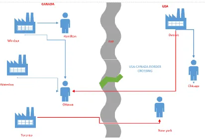
𝑖,𝑡Parameter is used to incorporate the customer demand for each time period into our model.Every facility can supply every customer, irrespective of its location (USA or Canada). When
a facility transports goods within the country, it uses domestic routes and incurs only domestic
cost of transportation. On the other hand when a facility transports goods to its customers across
border, it has to ship via cross border routes. In such scenario there is an extra cost incurred (𝑒𝑠)
due to disruption at cross border. As per the law, every manufacturing facility should maintain
2
CO emission below permissible limits. Hence, we include emission constraint to restrict total
24
Objective of the thesis is to minimize cost of entire supply chain by finding optimum quantity
of goods to be produced and shipped (𝑧𝑗,𝑖,𝑠,𝑡). Also, it aims to find instances at which there is a
need to construct/dismantle a capacity at any given facility.
Following map give a pictorial representation of cross border supply chain
25
3.2
Assumptions
Following assumption are made while developing ILP model:
1. At any facility, only one capacity can be constructed/dismantled at any given time
period.
2. Number of existing customers and facilities are known.
3. A facility is considered as a supplier. Supplier directly supplies to customer.
4. Facility locations are fixed and do not change over the planning horizon. Each facility has
to have an initial default existing capacity.
5. A single facility can supply to multiple customers.
6. We assume that inventory is either 0 or fixed at the end of time period. Inventory
parameter being constant is hence excluded. All goods produced are shipped to the
customers. Neither facility nor do customers have inventory.
7. Annual customer demand is considered to be deterministic and changes over the period
of time
8. Border crossing disruptions in supply chain are associated with scenario.
9. It is assumed that each facility uses green technology for manufacturing goods.
10. Only one capacity can be constructed from the available set of capacities at any time period for any particular facility.
11. Only one capacity can be dismantled from the available set of capacities at any time period for any particular facility
12. Orders for parts are placed at the start of the planning horizon, when all customer orders for products are known
13. All parts ordered from a supplier are shipped together in a single delivery
26