University of Windsor University of Windsor
Scholarship at UWindsor
Scholarship at UWindsor
Electronic Theses and Dissertations Theses, Dissertations, and Major Papers
10-7-2019
Green Supply Chain Network Design
Green Supply Chain Network Design
Penelopi Tatiana Krikella University of Windsor
Follow this and additional works at: https://scholar.uwindsor.ca/etd
Recommended Citation Recommended Citation
Krikella, Penelopi Tatiana, "Green Supply Chain Network Design" (2019). Electronic Theses and Dissertations. 7816.
https://scholar.uwindsor.ca/etd/7816
This online database contains the full-text of PhD dissertations and Masters’ theses of University of Windsor students from 1954 forward. These documents are made available for personal study and research purposes only, in accordance with the Canadian Copyright Act and the Creative Commons license—CC BY-NC-ND (Attribution, Non-Commercial, No Derivative Works). Under this license, works must always be attributed to the copyright holder (original author), cannot be used for any commercial purposes, and may not be altered. Any other use would require the permission of the copyright holder. Students may inquire about withdrawing their dissertation and/or thesis from this database. For additional inquiries, please contact the repository administrator via email
Green Supply Chain Network Design
by
Penelopi Tatiana Krikella
A Thesis
Submitted to the Faculty of Graduate Studies
through the Department of Mathematics and Statistics
in Partial Fulfillment of the Requirements for
the Degree of Master of Science at the
University of Windsor
Windsor, Ontario, Canada
2019
c
Green Supply Chain Network Design
by
Penelopi Tatiana Krikella
APPROVED BY:
—————————————————————–
A. Alfakih
Department of Mathematics and Statistics
—————————————————————–
E. Selvarajah
Odette School of Business
—————————————————————–
R. Caron, Advisor
Department of Mathematics and Statistics
Author’s Declaration of Originality
Abstract
Dedication
Acknowledgements
I would like to thank my thesis advisor Dr. Richard Caron, for his valuable and constructive suggestions during the development of this thesis. He was always available when I ran into a road block, or had any questions regarding my research or writing. His jokes and positive presence helped my stress levels throughout this year as well.
I would also like to acknowledge the help and support from my boyfriend, Will. Thank you for the countless hours of teaching me how to code in MatLab, and for supporting and encouraging me through the process of researching and writing. I could not have done this without you.
Finally, I must express my very profound gratitude to my parents and my friends for supporting me, and providing me with happy distractions when my research became too hectic. You all kept me sane.
Table of Contents
Author’s Declaration of Originality iii
Abstract iv
Dedication v
Acknowledgements vi
List of Figures viii
Chapter 1. Introduction 1
1.1. Scope and Motivation of Research 1
1.2. Chapter Structure 3
1.3. Optimization 4
1.3.1. Linear Programming 4
1.3.2. Classic Optimization Problems 7
1.3.3. Convexity 13
1.4. Penalty Methods and Lagrangian Relaxation 17
1.5. Decomposition 21
Chapter 2. Green Supply Chain Network Design 28
2.1. Introduction 28
2.2. Elhedhli and Merrick’s Model 29
2.3. Solution Strategy 31
2.4. Numerical Testing 42
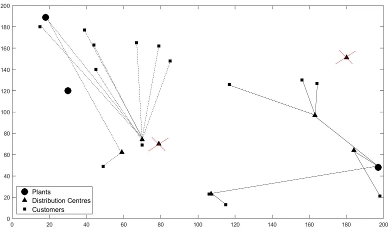
Chapter 3. Results and Findings 46
3.1. Introduction 46
3.2. Results and Findings 47
Chapter 4. Conclusions 51
4.1. Conclusion 51
4.2. Summary of Contributions 51
4.3. Future Work 52
Bibliography 53
Appendix A 55
Problem Reformulations for CPLEX Compatibility 55
List of Figures
1.1 A Transportation Problem 9
1.2 An Assignment Problem 10
1.3 A Facility Location Problem 12
1.4 The Lagrangian Function 20
1.5 An Optimization Problem with Complicating Constraints 21
2.1 Vehicle weight vs. CO2 emissions at 100km/h 43
3.1 Network Design with Zero Emissions Costs 48
3.2 Network Design with Moderate Emissions Costs 49
CHAPTER 1
Introduction
1.1. Scope and Motivation of Research
With the globalization of supply chains, the distances traveled has grown con-siderably, which in turn has increased the amount of daily vehicle emissions. As of 2019, transportation via combustion engine vehicles accounted for 28% of the Canadian greenhouse gas (CHG) inventory [2]. Integrating environmental costs into supply chains is now prevalent as we are realizing the effect carbon emissions have on the planet.
In their paper, Elhedhli and Merrick [1] develop a green supply chain design model which considers the cost of carbon emissions, in addition to fixed costs and trans-portation costs. Their proposed supply chain network is a three echelon model, which means it includes three levels: plants, DCs and customers. The goal of their supply chain network is to find the optimal locations of distribution centres (DCs), as well as the optimal assignments of plants to DCs and DCs to customers, which minimizes the overall cost of the network. Elhedhli and Merrick use published experimental data to derive a function that represents emissions costs. Their re-sulting model, a mixed integer programming problem, is the minimization of a concave function, which is a computationally difficult problem [3]. To solve the problem, the Lagrangian relaxation method is used which allows the problem to be decomposed into subproblems. The characteristics of the original problem are present in the subproblems, which results in achieving a strong Lagrangian bound. Elhedhli and Merrick then propose a primal heuristic to generate feasible solutions to their original problem. Their paper ends with numerical testing, in which they generate problems to test if their proposed method is effective in finding good solutions.
1.2. Chapter Structure
In this chapter, we introduce multiple concepts over three sections that are refer-enced in Elhedhli and Merrick’s problem formulation and solution strategy.
Section 1.3 is an overview of some concepts in optimization. It consists of three subsections. Subsection 1.3.1 covers linear programming. In this section, we dis-cuss basic notation and definitions, the Simplex method, duality theory and the necessary and sufficient conditions of optimality. Subsection 1.3.2 provides some details on three classic optimization problems: the transportation problem, the assignment problem, and the facility location problem. Each description includes a general problem, an example, a graph and a solution algorithm. Subsection 1.3.3 presents definitions and theorems related to convexity.
Section 1.4 provides information that may help in understanding the solution strat-egy of Elhedhli and Merrick. In their paper, Elhedhli and Merrick use Lagrangian relaxation as a tool to solve their model. This section includes the theory behind the exterior penalty method, the exact penalty method, as well as the Lagrangian relaxation technique.
1.3. Optimization
1.3.1. Linear Programming. The source of the material in this section is Best and Ritter’s [4].
Consider the general linear programming problem (LP), which is to find the values
xPRn that will
pLPq min z cJx (1)
s.t. Ax b, (2)
x¥0. (3)
We refer to (1) as the objective function. This is the function we are trying to minimize the value of, with respect tox. To solve the problem,x must satisfy the constraints represented by (2) and (3).
Definition 1.1. At a given point ˆx, a constraint can either be violated, satisfied
and inactive or satisfied and active.
(1) The constraint aJi x¤bi is violated at ˆx if aJi xˆ¡bi.
(2) The constraint aJi x¤bi is satisfied and inactive at ˆx if aJi xˆ bi.
(3) The constraint aJi x¤bi is satisfied and active at ˆxif aJi xˆbi.
(4) The constraint aJi xbi is violated at ˆx if aJi xˆbi.
(5) The constraint aJi xbi is satisfied and active at ˆxif aJi xˆbi.
We denote the feasible region as R tx P Rn | Ax b, x ¥ 0u. If x P R, we
say xis a feasible solution. An optimal solution is a feasible solution x such that
cJx ¤cJx,@xPR. When solving an LP, we are looking for the optimal solution.
In a linear program, there may exist redundancy in terms of the constraints. A con-straint gkpxq ¤ 0 is redundant in the feasible region R tx P Rn |gipxq ¤0,@iu
if tx P Rn |gipxq ¤ 0,@iu tx P Rn |gipxq ¤ 0,@i ku. In other words, a
con-straint is redundant if it is implied by other concon-straints. By including redundant constraint in a linear program, the computational effort of solving the program is affected, as time is wasted. We try to eliminate redundant constraints by removing them from the linear programming problem.
Each constraint of (LP) has a corresponding dual variable. We will denote the vector of dual variables associated with (2) and (3) by u, and v, respectively. We definev, the vector of dual variables associated with the non-negativity constraints, to be the reduced cost.
The gradient of a function is the vector of first partial derivatives. We will refer toai as the gradient of the ith constraint. The gradient of the objective function
isc.
Lemma 1.2. The negative gradient of the objective function, c, points in the
direction of maximal local decrease of the objective function z cJx.
Definition 1.3 (Extreme Point). The point ˆx P R is an extreme point of R if
A result used in LP solution algorithms is if there is an optimal solution, then there exists an extreme point that is an optimal solution. This result is used in the Simplex algorithm, which is a popular solution algorithm for an LP. To use the Simplex algorithm, the LP must be in the same form as (1)-(3) . This is called the Standard Simplex Form. The Simplex algorithm has two phases. In Phase I, we consider a ”relaxed” problem in which artificial variables are added to each of the constraints. An artificial variable is one that is required to be 0, but in Phase
I this requirement is relaxed, and the artificial variables are greater than or equal to 0. In this phase, there are two possible results: either all of the artificial vari-ables are eliminated, or we cannot eliminate all of them. If they are all eliminated, then an extreme point is found and PhaseII begins with that extreme point as a starting point. This phase also has two possible results: either an optimal solution is found, or we find that the objective function is unbounded from below.
An important topic in linear programming is duality theory. The Standard Simplex linear program given in (1)-(3) is called the primal. We define the dual of (1)-(3) to be the LP
pDLPq max bJu (4)
s.t. AJu¥ c (5)
Together, the two LPs are the primal-dual pair. Every linear programming problem has a corresponding dual problem. A relationship between the primal-dual pair is described in Theorem 1.4.
Theorem 1.4. The dual of the dual is the primal.
Proof. The dual of (1)-(3) is the LP
max bJu
s.t. AJu¥ c
which is equivalent to
min bJu
s.t. AJu¤c.
Now, the dual of the dual is
max cJy
Letyx, and substitute into the above LP to get
max cJx
s.t. Ax b,
x¥0 which simplifies to
min cJx
s.t. Axb, x¥0.
There is also a relationship between the objective functions of the primal and its dual.
Theorem 1.5 (Weak Duality). If xˆ is primal feasible and uˆ is dual feasible, then
cJxˆ¥ bJuˆ.
Proof. We use the primal (1)-(3) and its dual (4)-(5). From dual feasibility
we have
AJuˆ¤c. (6) and from primal feasibility we have ˆx¥0. We rewrite (6) as
cJ ¥ uJA
and post multiply by ˆx to get
cJxˆ¥ uJAx.ˆ (7) From primal feasibility we have
Axˆb. (8)
We pre-multiply (8) byuˆJ to get
uˆJAxˆ uˆJb. (9) Combining (7) and (9) we get the result
cJxˆ¥ bJu.ˆ
Theorem 1.6. Consider the LP min{cJx | Ax b, x ¥ 0}. The point x is an
optimal solution to this LP if and only if there exists a vector u that, together with x satisfy
(1) Axb, x¥0 (Primal Feasibility) (2) AJuv c, v ¤0 (Dual Feasibility) (3) vJx0 (Complementary Slackness) We proof the sufficiency of these conditions.
Proof. Suppose there are vectors x, u and v which satisfy the optimality
conditions in Theorem 1.6. We will show thatx is optimal for min{cJx|Axb,
x ¥0}. Since Ax ¤b, x ¥ 0, we know that x is feasible. Let ˆx be any other feasible point. We will show thatcJx ¤cJxˆ, i.e., that cJpxxˆq ¤0.
From dual feasibility, we have that
AJuv c,
ùñ cJ uJAJv.
Consider
cJpxxˆq puJAJvqpxxˆq,
puJAxvJxq puJAxˆvJxˆq,
uJAxuJAxˆvJx,ˆ by Complementary Slackness,
uJpAxAxˆq vJx,ˆ
uJpbbq vJx,ˆ by Primal Feasibility, vJx.ˆ
We have
v ¤0ˆx¥0
from dual feasibility, and the feasibility of ˆx, respectively.
So, we conclude that
cJpxxˆq vJx,ˆ
¤0.
1.3.2. Classic Optimization Problems. The source for the material in this section is Ahuja et al.’s [11].
Definition 1.7. A graph is an ordered pair, G pN, Aq, where N is a set of
nodes (also called vertices) and A is a set of arcs. A directed graph is a graph in which the arcs begin at a location, i, and end at a location, j. We denote this directed arc as (i, j). A directed graph can also be called a directed network.
Throughout this chapter, the graphs/networks we discuss are all directed graphs/networks.
A transportation problem is a directed network where the node set N is parti-tioned into two subsets N1 and N2, not necessarily equal in size. Each node in
N1 is a supply node, each node in N2 is a demand node and for each arc pi, jq in
the network, i P N1 and j P N2. The variable xij represents the number of units
flowing over arcpi, jq. Further, each arcpi, jqhas an associated per unit flow cost,
cij.
A general transportation model is to
pT Mq min
n
°
i1
m
°
j1
cijxij
s.t.
m
°
j1
xij ai, @i1, ..., n n
°
i1
xij bj @j 1, ..., m
lij ¤xij ¤uij @pi, jq
xij PZ, @pi, jq
The transportation problem, (TM), is a balanced transportation problem. A trans-portation model is balanced if
n
¸
i1
ai m
¸
j1
bj.
Property 1.8. A transportation problem will have feasible solutions if and only
if the problem is balanced (Hillier and Lieberman, [6]).
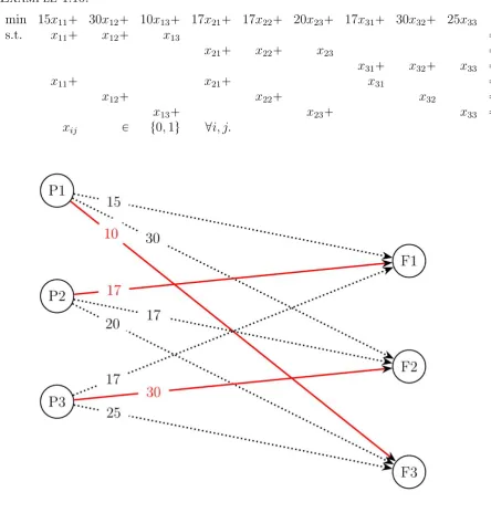
Example 1.9 shows a balanced transportation problem, along with its graph rep-resented by Figure 1.1 and its solution.
Example 1.9.
min 15x11 10x12 11x13 17x21 8x22 15x23
s.t. x11 x12 x13 100
x21 x22 x23 200
x11 x21 75
x12 x22 175
x13 x23 50
xij ¥ 0 i1,2, j 1,2,3 .
The nodes on the left, P1 and P2, are the supply nodes. The nodes on the right,
F1, F2 and F3, are the demand nodes. The capacities of both supply and demand
nodes are displayed outside of the nodes. The unit cost associated with each arc
Figure 1.1. A Transportation Problem
arc. If an arcpi, jq is represented by a dotted line, then there is no product being shipped on that arc.
The transportation problem can be solved using the transportation simplex method. This method avoids the use of artificial variables, which in turn avoids the (n+m-1) iterations to eliminate them.
An assignment problem is a special case of the transportation problem in which
ai bj 1,@i, j and xij P t0,1u,@i, j. A general model of an assignment problem
is
pAMqmin
n
°
i1
m
°
j1
cijxij
s.t.
m
°
j1
xij 1, @i1, ..., n n
°
i1
xij 1, @j 1, ..., m
xij P t0,1u @i, j.
The constraints of the assignment problem ensure that each supply node, i, is assigned to only one demand node, j. Also, each demand node j is only assigned to one supply node,i. Finally, in an assignment problem, the variables are binary. The variable,xij is 1 if node i is assigned to node j, and 0 otherwise.
Example 1.10.
min 15x11 30x12 10x13 17x21 17x22 20x23 17x31 30x32 25x33
s.t. x11 x12 x13 1
x21 x22 x23 1
x31 x32 x33 1
x11 x21 x31 1
x12 x22 x32 1
x13 x23 x33 1
xij P t0,1u @i, j.
Figure 1.2. An Assignment Problem
If the arc, pi, jq, is represented by a dotted line, then the Pi is not assigned to Fj
. The values on each arc pi, jqis the unit cost associated with that arc.
A well known algorithm to solve assignment problems is the Hungarian algorithm. This algorithm terminates withinn1 iterations, where n1 is the number of supply
nodes. In the example above, the algorithm would terminate within 3 iterations.
capacitated facility location problem.
Consider n facilities and m customers. Let hjk be the transportation cost from
facility i, i 1, ..., n to customer j, j 1, ..., m. Let gi denote the fixed cost of
opening facility i. Let vj be the capacity for facility j. Let dk be the demand of
customer k. Let zj be the binary variable where xi 1 if facility i is open, and
0 otherwise. Let xjk be the number units shipped from facility j to customer k.
These variables and indices are consistent with those in the model proposed by Elhedhli and Merrick, which is described in Chapter 2.
Then, the capacitated facility location problem is given by
pF LPq min
n
¸
j1
m
¸
k1
hjkxjk n
¸
i1
gjzj (10)
s.t.
n
¸
j1
xjk dk @k (11)
m
¸
k1
xjk ¤vjzj @j (12)
zj P t0,1u @j (13)
xjk PZ¥0 @j, k. (14)
The symbol Z¥0 represents the space of non-negative integers. Constraint (11)
ensures customer demand is satisfied. Constraint (12) ensures that the units being shipped from a facility j never exceeds the capacity of the facility j. Constraints (13) and (14) definezj to be a binary variable and xjk to be a non-negative
inte-ger, respectively. If each customer is sourced by one facility, we say that the above problem has single sourcing.
Example 1.11 shows a capacitated facility location problem, along with its graph represented by Figure 1.3 and its solution.
Example 1.11. Consider a system with three distribution centres (DCs) and five
customers. We wish to determine which DCs should open, as well as how much product is going from each DC to each customer to satisfy the demand of each customer.
Letj 1,2,3 index the DCs, and let k1, ...,5 index the customers.
Let
rhjks
50 75 100 100 3070 70 85 100 50 55 60 60 120 45
,rgjs
120100
100
,rvjs
250200
200
,rdks
Then, we want to
min
3
°
j1 5
°
k1
hjkxjk
3
°
j1
gjzj
s.t.
3
°
j1
xjk dk @k
5
°
k1
xjk ¤ vjzj @j
zj P t0,1u @j
xjk ¥ 0 @j, k.
Figure 1.3. A Facility Location Problem
shipped on that arc. We do not include the unit costs of shipping on an arc in the graph as to avoid clutter. From the solution, we see that DC2 is not open.
As the capacity facility location problem is an integer programming problem, al-gorithms used to solve integer programming problems can be used. An example of such an algorithm is the Branch and Bound method. This procedure involves searching for an optimal solution by partitioning the feasible region into subsets (branching), then pruning the enumeration by bounding the objective function values of the subproblems generated [7].
1.3.3. Convexity. The source for the material in this section is Rockafellar’s [8].
We begin with the definitions of a convex set and a convex combination.
Definition 1.12. A subset C of Rn is convex ifp1λqx λy P C whenever xP
C,yP C and 0 λ 1.
A convex set C is closed if it contains all of its limit points.
Example1.13.Consider the Standard Simplex linear programming problem given
in (1)-(3). We will show that the feasible regionR tx PRn | Axb, x ¥0u is a convex set.
Letx1, x2 PR and let λP r0,1s. Since Ax1 b and Ax2 b then
App1λqx1 λx2q Ap1λqx1 Apλx2q
p1λqAx1 λAx2
p1λqb λb
b.
Sincex1 ¥0 and x2 ¥0, we have
p1λqx1 λx2 ¥0
Definition 1.14. A convex combination of vectorsy1, ..., yn is their linear
combi-nation
y
n
¸
i1
λiyi
with non-negative coefficients with unit sum, that is,
λi ¥0, n
¸
i1
λi 1
A line is uniquely determined by a point and a vector. For example,
x λs, λPR
represents a line, from pointx, extending in directionss. A line extends in both directions infinitely. A half line, or a ray, is a line which extends in only one direction. For example,
x λs, λ¥0
is a ray. A line segment can be expressed by the convex combination of any two points in Rn. For example,
p1λqx1 λx2,0¤λ¤1
is the line segment connectingx1 and x2.
To conclude our discussion of convex sets, we introduce some topological definitions that will be used in Chapter 2 of this thesis.
Definition1.15. Let C be a non-empty convex set inRn. We say that C recedes in the directiony 0 if and only if x λyP C for every λ¥0 andxPC. The set of all vectors y satisfying these conditions, including y0, is called the recession cone of C and is denoted by 0 C
Definition 1.16. Let C be a non-empty convex set. The set p0 Cq X0 C is
called the lineality space of C. It consists of the zero vector and all the non-zero vectors y such that, for every x P C, the line through x in the direction of y is contained in C.
We begin our overview of convex functions with the following definitions:
Definition 1.17. Let f be a function whose values are real or 8 and whose
domain is a subset S of Rn. The epigraph of f, denoted by epif, is the set
tpx, µq|xPS, µ PR, µ¥fpxqu.
We define f to be a convex function on S if the epif is a convex set. A concave function on S is a function whose negative is convex.
Definition 1.18. The effective domain of a convex function f on S, denoted by
domf, is the set
tx|fpxq 8u.
The dimension of domf is called the dimension of f.
Definition 1.19. Let C be a non-empty convex set. The function f : C Ñ R is convex if and only if
fpp1λqx λyq ¤ p1λqfpxq λfpyq0¤λ¤1,
for every x and y in C.
Definition 1.20. The function f : CÑR is convex if and only if
fpp1λqx λyq ¥ fpxq λp5xfpxqpyxqq
whenever λ¥0 and x, y P C.
Definition 1.21. Let f be a twice differentiable real-valued function on an open
convex set C in Rn. Then f is convex on C if and only if its Hessian matrix is
positive semi-definite for everyxP C.
Examples 1.22 and 1.23 show how we can prove functions are concave and/or convex.
Example 1.22. To show that fpxq alnpxq b,a ¡0, is concave on its domain,
p0,8q, we show that it’s negative is convex using Definitions 1.21. Since we are in R1, we do not need to find the Hessian, we can simply take the second derivative of the function. If the value of the second derivative is negative for all values ofx, then the function fpxq is concave on its domain.
dfpxq dx
a x d2fpxq
dx2
a x2
The negative of the second derivative will always be positive for values ofxgreater than 0, thus showing that fpxq is convex on its domain. Therefore, fpxq is concave on its domain.
Example 1.23. From Definition 1.21, we know that if the second derivative of
a function, fpxq, is equal to 0 for all values of x, then fpxq is both concave and convex. We will show that the linear function function fpxq mx b is both concave and convex.
dfpxq dx m d2fpxq
dx2 0
Theorem 1.24. Let f be a convex function and let C be a closed, convex set
con-tained in the domf. Suppose there are no half lines in C on whichf is unbounded above. Then
suptfpxq|xPCu suptfpxq|xP Eu
where E is the subset of C consisting of the extreme points of CXLK, L being the lineality space of C. The supremum relative to C is attained only when the supremum relative to E is attained.
The proof of this theorem is omitted as we are more interested in its corollary.
Corollary 1.25. Let f be a convex function and let C be a closed convex set
contained in domf. Suppose that C contains no lines. Then, if the supremum of
f relative to C is attained at all, it is attained at some extreme point of C.
Proof. If C contains no lines, then L={0} and C XLK C. By Theorem
1.24, E is the set containing extreme points of C XLK C. Thus, E is the set containing extreme points of C. Further, the supremum relative to C is attained only when supremum relative to E is attained. As follows, the supremum of f
1.4. Penalty Methods and Lagrangian Relaxation
The source for the material on penalty methods is Avriel’s [9].
Suppose we want the minimum of a real-valued, continuous functionf, defined on Rn, on a proper subset X of Rn.
Define
Ppxq
#
0 xP X
8 otherwise.
Ppxqis called the penalty function, as it imposes an infinite penalty on points out-side of the feasible set. Conout-sider the unconstrained minimization of the augmented objective function, F, given by
minFpxq fpxq Ppxq.
A point x minimizes F if and only if it minimizes f over X. Solving the uncon-strained minimization ofF cannot be carried out in practice because of the infinite penalty on values outside of X. Instead, penalty methods consist of solving a se-quence of unconstrained minimizations in which a penalty parameter is adjusted from one minimization to another, so that the sequence converges to an optimal point of the constrained problem. There are many different penalty methods, but we will discuss the exterior and the exact penalty method.
Consider the general non-linear programming problem
min fpxq
s.t. gipxq ¥ 0 i1, ..., m
hjpxq 0 j 1, ..., p
(15)
wherefpxq, gipxqand hjpxq are continuous @i1, ..., n, j 1, ..., n. Let S denote
the feasible set. The exterior penalty method, which is mainly useful for convex programs, solves (15) by a sequence of unconstrained minimization problems that converge to an optimal solution of (15) from outside of the feasible set. In the sequence, a penalty is imposed on every x outside the feasible set such that the penalty is increased from problem to problem, forcing the sequence to converge towards to feasible set.
To develop the algorithm, define the real-valued, continuous functions
ψpηq |minp0, ηq|α
and
ζpηq |η|β, ηPR
Let
spxq
m
¸
i1
ψpgipxqq p
¸
j1
ζphjpxqq
be the loss function for problem (15). Note that
spxq 0 if xPS spxq ¥ 0 otherwise.
For anyp¡0, we define the augmented objective function for problem (15) as
Fpx, pq fpxq 1 pspxq.
It is noted that Fpx, pq fpxq if and only if x is feasible. Otherwise, Fpx, pq ¡ fpxq.
The exterior penalty method consists of solving a sequence of unconstrained opti-mizations for k0,1,2, ...given by
min
x Fpx, p
kq fpxq 1
pkspxq (16)
using a strictly increasing sequence of positive numbers,pk. Letxkbe the optimal
solution to the kth unconstrained optimization. The point xk is the initial point
in the algorithm to solve (16). Then, the sequence of points txku, under mild
conditions on (15), has a subsequence that converges to an optimal point of (15).
The exterior penalty method described is one of many that solves a sequence of unconstrained optimization problems to find the optimal solution of a non-linear programming problem. Another method that can be used to solve a non-linear programming problem, that doesn’t require solving a sequence of optimization problems, is Lagrangian relaxation. This relaxation technique consists of embed-ding at least one of the constraints into the objective function with an associated Lagrangian multiplier µ, thus relaxing the constraint(s). The Lagrangian mul-tipliers are simply the dual variables associated with the constraints. When a constraint is relaxed, it need not be satisfied, but a violation of the constraint penalizes the solution. The new, relaxed problem is then solved subject to the re-maining constraints. Unlike the exact penalty method, the solution to a problem in which Lagrangian relaxation is applied is not an optimal solution of the original problem, but is still useful as bounds on the optimal solution can be determined.
The source for the material on Lagrangian relaxation is Ahuja et al.’s [11] and Conejo et al.’s [12].
Consider the Standard Simplex linear programming problem, (1)-(3).
We relax constraint (2). The new problem after applying Lagrangian relaxation is
min z cJx µJpAxbq (17)
In the problem given in (17)-(18), µ is the fixed vector of Lagrangian multipliers, which can be positive or negative, and has the same dimensions as the vector b. The Lagrangian multipliers are the dual variables associated with the constraints being relaxed. When Ax b , x is not in the feasible region and the Lagrangian term in the objective function acts as a penalization. If the relaxed constraint is an inequality constraint, then the vector of Lagrangian multipliers would have to be all non-negative entries.
The function
Lpµq mintcJx µpAxbq:x¥0u (19) is referred to as the Lagrangian function.
Although the solution found from the relaxation is not optimal, a lower bound of the optimal value of (1) can be determined which gives useful information about the original problem.
Lemma1.26 (Lagrangian Bounding Principle). For any vectorµof the Lagrangian
multipliers, the valueLpµq of the Lagrangian function (19) is a lower bound on the optimal objective function value, z, of the original optimization problem given in (1)-(3).
Proof. Since Ax b for every feasible solution to the problem given in
(1)-(3), for any vectorµ of Lagrangian multipliers,
z mintcJx:Axb, x¥0u (20)
mintcJx µpAxbq:Axb, x¥0u. (21) Since removing the constraintsAxb from (21) cannot lead to an increase in the value of the objective function,
z ¥mintcJx µJpAxbq:x¥0u ðñ z ¥Lpµq.
SinceLpµqis a lower bound on the optimal objective function value for any value of µ, the sharpest, or best, possible lower bound is found by solving the following optimization problem
L max
µ Lpµq. (22)
This optimization problem is referred to as the Lagrangian multiplier problem (also called the dual problem) associated with the problem given in (1)-(3). Applying the Weak Duality Theorem, we have that the optimal objective function value
L of (22) is always a lower bound on the optimal value of (1). In other words,
L ¤ z. Then, for any Lagrangian multipliers µ, and any feasible solution x of the problem given in (1)-(3), we have
Lpµq ¤ L ¤z ¤cJx.
cJx µJpAxbq as the composite cost of x. If the set X tx1, ..., xvu is finite, then by definition,
Lpµq ¤cJxr µJpAxrbq @r1, ..., v.
In the space of composite costs and Lagrangian multipliers,µ, each function yr
cJxr µJpAxrbqis a hyperplane. By definition of a hyperplane, its dimension is
exactly one less than the dimension of the whole space. The Lagrangian function, (19), is the lower envelope of these hyperplanes forr1, ..., k. We give a visual of this lower envelope in Figure 1.4. This visual is based on an example found in [11]. The optimization problem it is based on is not relevant to this section. We only include the graph of the composite costs to show how (19) is the lower envelope of the composite cost hyperplanes.
Figure 1.4. The Lagrangian Function
The bold, concave line in Figure 1.4 represents the Lagrangian function, (19). In the Lagrangian multiplier problem, (22), we wish to determine the highest point of (19). This point can be found by solving the Lagrangian master problem, given in (23)-(24).
max w (23)
s.t. w¤cJxr µJpAxrbq @r1, ..., v (24) This result is stated as a theorem.
Theorem 1.27. The Lagrangian multiplier problem L maxµLpµq with Lpµq
mintcJx µJpAxbq : x ¥ 0u is equivalent to the linear programming problem
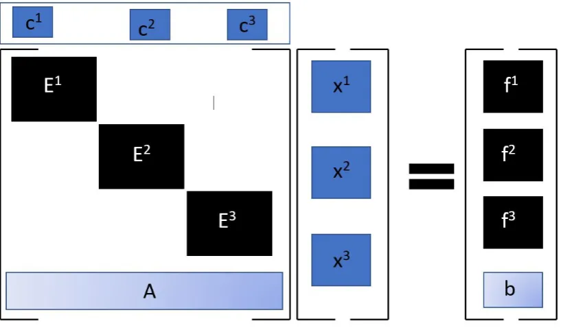
1.5. Decomposition
The ideas in the section are based on the material by Conejo’s et al. [12].
To begin the section, suppose an optimization problem has the structure shown in Figure 1.5.
Figure 1.5. An Optimization Problem with Complicating Constraints
In Figure 1.5, the top rectangle with blocks c1, c2 and c3 represents the objective function. The equation below the objective function is representative of the con-straints of the optimization problem. If we ignore the block of concon-straintsAxb, we see that the constraints have a staircase structure. That is, the problem can be decomposed into subproblems of the form
min ckJxk
s.t. Ekxkfk
for each k 1,2,3.
We now generalize this concept. Consider the following problem
min cJx (25)
s.t. Exf (26)
Ax b (27)
x¥0. (28)
In this problem, x is an pn1q vector. The matrices E and A are pq nq and
pmnq, respectively. Constraint (26) can be decomposed into r blocks, each of size pqknkq, where k 1, ..., r. Constraint (27) is the complicating constraint.
It does not have a decomposable structure. Constraint (28) sets a lower bound on the variables.
If the complicating constraint is ignored (relaxed), then the problem given in (25)-(28) becomes
min cJx (29)
s.t. Exf (30)
x¥0. (31)
The problem given in (29)-(31) can now be decomposed intok subproblems. The
kth subproblem is
min crksJxrks (32)
s.t. Erksxrks frks (33)
xrks ¥0. (34)
Example 1.28. The problem
min 10x1 4x37x5
s.t. x1 x2 10
x3 x4 8
x5 x6 1
x1 x3 x6 11
xi ¥0 @i1, ...,6
has a decomposable structure into three blocks, where the last equality
x1 x3x6 11
is the complicating constraint. The relaxed problem would be
min 10x1 4x37x5
s.t. x1 x2 10
x3 x4 8
x5 x6 1
The three blocks would be:
min 10x1
s.t. x1 x2 10
x1, x2 ¥0,
min 4x3
s.t. x3 x4 8
x3, x4 ¥0
and
min 7x5
s.t. x5x6 1
x5, x6 ¥0.
Suppose each subproblem is solvedptimes with different, arbitrary objective func-tions. Assume that thep basic feasible solutions of the problem given in (29)-(31) are
X
xp11q xp12q xp1pq xp21q xp22q xp2pq
..
. ... . .. ...
xpn1q xpn2q xpnpq
.
wherexpjsq is the jth component of solution s,j 1, ..., n and s1, ..., p.
The correspondingp optimal objective function values are
z
zp1q zp2q
.. .
zppq
wherezpsq is the objective function value of solution s.
The values of the m complicating constraints for the above p solutions are found by multiplying the matrix Amn by the matrixXnp. The resulting m values are
Rmp AX
rp11q r1p2q rp1pq rp21q r2p2q rp2pq
..
. ... . .. ...
rpm1q rmp2q rpmpq
.
where ripsq is the value of the ith complicating constraint for the sth solution,
Example 1.29. Applying the above to Example 1.28, suppose we solve each
sub-problem p2 times, and we get the following solutions
xp1q
10 0 8 0 1 0
, xp2q
10 0 0 8 0 1 .
Then, we have
X 10 10 0 0 8 8 0 0 1 0 0 1 , z 75 100 .
The values of the complicating constraints are
R 18 17 .
To derive the master problem, we use the fact that a linear convex combination of basic feasible solutions of a linear program is a feasible solution of that linear program. This is true because the feasible region of a linear program is convex, which we showed in Example 1.13. The proof is trivial, so it is omitted.
We now solve the master (weighting) problem
min zJu (35)
s.t. Rub; λ (36)
eJu1; σ (37)
u¥0 (38)
whereuis a (p1) column vector of weights,eis a (p1) column vector of 1’s,λ
is the vector of dual variables corresponding to constraint (36) andσ is the vector of dual variables corresponding to constraint (37). The goal of the problem is to find the value of u which minimizes the value of all convex combinations of the p
basic feasible solutions. Constraint (36) ensures that the complicating constraints of the original problem are enforced. Constraints (37) and (38) ensure that the weighting vectoru satisfies the convex combination requirements.
A solution to the problem given in (35)-(38) is a convex combination of the p
Example 1.30. Continuing our example, the master problem would be
min 75u1100u2
s.t. 18u1 17u2 11; λ
u1 u2 1; σ
u1, u2 ¥0.
Consider a prospective new basic feasible solution is added to the problem given in (35)-(38) with objective function value zj and complicating constraint values
r1, ..., rm.
The new master problem becomes
min
u,uj
z zj u uj
J
(39)
s.t.R rj
u uj
b; λ (40)
eJ
u uj
1; σ (41)
u uj
J
¥0 (42)
whereuj is the weight corresponding to the prospective new basic feasible solution.
Example 1.31. Now, let
x
10 0 0 8 0 1
be a new prospective feasible solution.
The corresponding objective function value of this solution is z 107, and its complicating constraint value is r11.
Then, our new master problem becomes
min 75u1100u2107u3
s.t. 18u1 17u2 11u3 11 λ
u1 u2 u3 1; σ
u1, u2, u3 ¥0.
The reduced cost ofuj can be computed as
dzjλJrj σ
pcj AλqJxj σ
where xj is the new prospective basic feasible solution. To find the minimum
reduced cost, we solve
min pcj AλqJxj (43)
s.t. Exj f (44)
xj ¥0 (45)
Theσ in the objective function is omitted since it is a constant. Constraint (44) is included to make the new basic feasible solution feasible in the original problem, (25)-(28). The problem given in (43)-(45) can be solved in blocks, as it has the same structure as the relaxed problem, (29)-(31), just a different objective function.
Example 1.32. The reduced cost associated with u3 is
d p1λqx1 p1λqx3 p1 λqx6.
To find the minimum reduced cost, we solve
mind
s.t.x1 x2 10
x3 x4 8
x5x6 1
xi ¥0 @i1, ...,6.
This can be decomposed into three subproblems, similar to what we did in Example 1.28.
Using the solutions from each of the subproblems, we solve the optimal value ofd, which we call v0.
Let
ν pcjAλqJxj
be the optimal value of [43]. Then,
d νσ
is the minimum reduced cost where σ is the optimal value of the dual variable associated with constraint (41).
If ν ¥ σ, the prospective basic feasible solution does not improve the reduced cost, so we do not include xj in the set of previous solutions. If ν σ, the
xj in the set of previous basic feasible solutions.
Example1.33. To conclude our example, if the reduced cost is negative, the basic
feasible solutionx is added to the set of previous basic feasible solutions. So, our matrix X would now be
X
10 10 10
0 0 0
8 8 0
0 0 8
1 0 0
0 1 1
.
Otherwise,x is not added to the matrix, X.
CHAPTER 2
Green Supply Chain Network Design
2.1. Introduction
In this chapter, we present Elhedhli and Merrick’s model and solution strategy.
Section 2.2 describes the problem formulation, and the assumptions that the model is based on. All variables and constants are defined, and the significance of the objective function and each of the constraints is described.
Section 2.3 outlines the strategies Elhedhli and Merrick used to find an optimal solution to the model introduced in Section 2.2. Lagrangian relaxation is used to relax the complicating constraint, thus allowing decomposition. A Lagrangian algorithm to find the best lower bound of the objective function from Section 2.2 is described. To find feasible solutions, a primal heuristic is then used. We show each step of the solution strategy.
2.2. Elhedhli and Merrick’s Model
This is a supply chain network design problem. The purpose of the problem is to find the optimal locations of the distribution centres (DCs), as well as the optimal assignments of plants to DCs and DCs to customers. This supply chain model is made up of three echelons, which are the levels in the supply chain: the plants, the DCs and the customers. Define the indices i 1, ...m, j 1, ..., n and k=1, ..., p
which correspond to plant locations, potential distribution centers (DCs) and cus-tomers, respectively. A DC at location j has a maximum capacity of Vj and a
fixed cost ofgj. Each customer has a demand of dk. The variable cost of shipping
a production unit from plant ito DC j is cij. Similarly, hjk is the variable cost of
shipping a production unit from DCj to customer k.
Letxij be the number of production units shipped from plant i to DC j. Let yjk
be 1 if customer k is assigned to DC j, and 0 otherwise. Let zj be 1 if a DC is
built at location j, and 0 otherwise.
Consider the mixed integer program
(FLM) min
m
¸
i1
n
¸
j1
fijpxijq n
¸
j1
p
¸
k1
fjkpdkyjkq m
¸
i1
n
¸
j1
cijxij (46)
n
¸
j1
p
¸
k1
hjkdkyjk n
¸
j1
gjzj
s.t.
n
¸
j1
yjk 1, @k, (47)
m
¸
i1
xij p
¸
k1
dkyjk, @j, (48)
m
¸
i1
xij ¤Vjzj, @j, (49)
p
¸
k1
dkyjk ¤Vjzj, @j, (50)
yjk, zj P t0,1u;xij ¥0, @i, j, k. (51)
The terms
m
°
i1
n
°
j1
fijpxijq and n
°
j1
p
°
k1
fjkpdkyjkq of the objective function, (46), are
measures of the carbon emissions from plantito DCj and from DCj to customer
k, respectively. The measure of carbon emissions is a function of the number of units being shipped and weight. This is because the number of units being shipped is directly proportional to the number of trucks needed for transportation. The subscripts on the functions correspond with where the trucks are travelling. The function fijpq is the emissions cost of a truck travelling from plant i to DC j.
Similarly, the function fjkpq is the emissions cost function of a truck travelling
The details of these functions are discussed in section 2.4. The terms
m
°
i1
n
°
j1
cijxij and n
°
j1
p
°
k1
hjkdkyjk of (46) are measures of the
transporta-tion cost from plant i to DC j and from DC j to customer k, respectively. The transportation cost is equal to the cost of shipping one unit multiplied by number of units being shipped. Both xij and dkyjk are flow variables, and represent the
number of units shipped in an echelon. The variablexij represents the number of
units shipped from planti to DCj . The variabledkyjk represents the number of
units shopped from DC j to customer k.
The term
n
°
j1
gjzj of (46) is a measure of the fixed cost of constructing DC j.
The objective function, (46), includes three costs: the emissions cost, transporta-tion cost and fixed cost.
We now analyze the constraints. Constraint (47) ensures that each customer is assigned to only one DC. Constraint (48) ensures that the flow of goods into the DC is equal to the flow of goods out of the DC. This constraint links the echelons in the network. Together, constraints (47) and (48) ensure that total customer demand is satisfied. From constraint (47), each customer is assigned to a DC, and from constraint (48), the number of units coming into the DC is guaranteed to satisfy the demand of the customers assigned to that DC. Constraint (49) provides an upper bound to the number of units shipped to a DCj, that upper bound being the capacity of DCj. Constraint (50) provides an upper bound to the number of units shipped to all customers of a DC j, that upper bound being the capacity of DC j. These two constraints, (49) and (50), ensure that the number of units entering and leaving a DCj never exceeds that capacity of DC j. Constraint (51) sets yjk and zj as binary variables, andxij as a non-negative variable.
2.3. Solution Strategy
Lagrangian relaxation is used on the problem given in (46)-(51) by relaxing con-straint (48). This constraint links the echelons of the supply chain, and is a complicating constraint.
Recall the objective function (46). Relaxing the complicating constraint (48) using the fixed vector of Lagrangian multipliersµj, we obtain:
m
¸
i1
n
¸
j1
fijpxijq n
¸
j1
p
¸
k1
fjkpdkyjkq m
¸
i1
n
¸
j1
cijxij n
¸
j1
p
¸
k1
hjkdkyjk n
¸
j1
gjzj
n
¸
j1
µjp m
¸
i1
xij p
¸
k1
dkyjkq
ðñ
m
¸
i1
n
¸
j1
fijpxijq n
¸
j1
p
¸
k1
fjkpdkyjkq m
¸
i1
n
¸
j1
cijxij n
¸
j1
p
¸
k1
hjkdkyjk n
¸
j1
gjzj
n
¸
j1
µj m
¸
i1
xij n
¸
j1
µj p
¸
k1
dkyjk
ðñ
m
¸
i1
n
¸
j1
fijpxijq n
¸
j1
p
¸
k1
fjkpdkyjkq m
¸
i1
n
¸
j1
cijxij n
¸
j1
p
¸
k1
hjkdkyjk n
¸
j1
gjzj
m
¸
i1
n
¸
j1
µjxij n
¸
j1
p
¸
k1
µjdkyjk
ðñ
m
¸
i1
n
¸
j1
fijpxijq n
¸
j1
p
¸
k1
fjkpdkyjkq m
¸
i1
n
¸
j1
pcijxij µjxijq
n
¸
j1
p
¸
k1
phjkdkyjk µjdkyjkq n
¸
j1
gjzj
ðñ
m
¸
i1
n
¸
j1
fijpxijq n
¸
j1
p
¸
k1
fjkpdkyjkq m
¸
i1
n
¸
j1
pcij µjqxij
n
¸
j1
p
¸
k1
phjkdk dkµjqyjk n
¸
j1
gjzj
The new mixed integer program can now be written as
(LR-FLM) min
m
¸
i1
n
¸
j1
fijpxijq n
¸
j1
p
¸
k1
fjkpdkyjkq m
¸
i1
n
¸
j1
pcij µjqxij (52)
n
¸
j1
p
¸
k1
phjkdk dkµjqyjk p
¸
k1
gjzj
s.t.
n
¸
j1
yjk 1 @k
(53)
m
¸
i1
xij ¤Vjzj @j
(54)
p
¸
k1
dkyjk ¤Vjzj @j
(55)
yjk, zj P t0,1u;xij ¥0 @i, j, k.
(56)
The purpose of applying Lagrangian relaxation to the original problem, (46)-(51), is to relax the complicating constraint. Now, the relaxed problem, given in (52)-(56), can be decomposed into subproblems. Specifically, it is decomposable by echelon.
The first subproblem is in terms of the binary variables yjk and zj. The solution
of the problem determines the assignment of customers to DCs, and which DCs will open. We define (57)-(60) to be the first subproblem.
min
n
¸
j1
p
¸
k1
fjkpdkyjkq n
¸
j1
p
¸
k1
phjkdk dkµjqyjk p
¸
k1
gjzj (57)
s.t.
n
¸
j1
yjk 1 @k (58)
p
¸
k1
dkyjk ¤Vjzj @j (59)
yjk, zj P t0,1u @i, j, k. (60)
The first term in the objective function is the emissions cost, the second is the transportation and shipping cost from DC j to customer k, and the last term is the fixed cost of opening a DC at location j. We know that yjk is binary, and
n
°
j1
function of the above problem (57).
n
¸
j1
p
¸
k1
fjkpdkyjkq n
¸
j1
p
¸
k1
phjkdk dkµjqyjk p
¸
k1
gjzj
ðñ
n
¸
j1
p
¸
k1
fjkpdkqyjk n
¸
j1
p
¸
k1
phjkdk dkµjqyjk p
¸
k1
gjzj
ðñ
n
¸
j1
p
¸
k1
pfjkpdkqyjk phjkdk dkµjqyjkq p
¸
k1
gjzj
ðñ
n
¸
j1
p
¸
k1
pfjkpdkq hjkdk dkµjqyjk p
¸
k1
gjzj (61)
Now, we may re-define the first subproblem with its new objective function, (61)
(SP1) min
n
¸
j1
p
¸
k1
pfjkpdkq hjkdk dkµjqyjk p
¸
k1
gjzj (62)
s.t.
n
¸
j1
yjk 1 @k (63)
p
¸
k1
dkyjk ¤Vjzj @j (64)
yjk, zj P t0,1u @i, j, k. (65)
The problem given in (62)-(65) is the first subproblem, and is a capacitated facility location problem with single sourcing.
The second subproblem is in terms of the flow variablexij, and its solution
deter-mines the number of units that will be shipped from each plant to a specific DC. We define (66)-(68) to be the second subproblem.
min
m
¸
i1
n
¸
j1
fijpxijq m
¸
i1
n
¸
j1
pcij µjqxij (66)
s.t.
m
¸
i1
xij ¤Vjzj @j (67)
xij ¥0 @i, j. (68)
min
m
¸
i1
fijpxijq m
¸
i1
pcij µjqxij (69)
s.t.
m
¸
i1
xij ¤Vjzj (70)
xij ¥0 @i. (71)
When zj 0, a DC is not built at location j, making that case trivial. If that
case is ignored, and we only consider the case whenzj 1, then problem (69)-(71)
becomes
min
m
¸
i1
fijpxijq m
¸
i1
pcij µjqxij (72)
s.t.
m
¸
i1
xij ¤Vj (73)
xij ¥0 @i. (74)
The objective function, (72), consists of the sum of concave functions, fijpxijq,
added to the sum of linear functions,pcijµjqxij. The sum of a concave functions
is still concave, and a linear function is a concave function. So, (72) is concave.
Recall Corollary 1.25. This corollary is applied to the problem given in (72)-(74) to show that a global solution of this problem is achieved at some extreme point of its feasible domain. LetCrepresent the feasible region of the problem given in (72)-(74).
In this problem, we know f, the emissions cost function, is concave. Recall that a line extends in both directions infinitely. Clearly, C contains no lines since the constraints are bounded below by 0. Since C is the feasible region of a linear programming problem, it follows from Example 1.13 thatCis a closed, convex set.
Since the problem given in (72)-(74) has an optimal solution at an extreme point of C, we look closely at the structure of the extreme points. The extreme points of
Care at points where at most onexij takes on the value of VJ, and the remaining
xij are equal to 0. This implies that the optimal solution will be at one of these
points. This allows us to reformulate the problem given in (72)-(74) as
(SP2j) min fijpVjq m
¸
i1
pcij µjqxij (75)
s.t.
m
¸
i1
xij ¤Vj (76)
xij ¥0 @i. (77)
computational effort relative to the original problem. Then subproblems given in (75)-(77) can be solved relatively quickly. The first subproblem, given in (62)-(65), retains important characteristics of the initial problem such as the assignment of all customers to a single warehouse, and the condition that the demand of all customers is satisfied. These characteristics are retained in the feasible region of (62)-(65). A drawback of the relaxation is that (62)-(65) is now a capacitated fa-cility location problem with single sourcing, which can be difficult to solve because the variables are binary. However, (62)-(65) is still easier to solve than the original problem, (46)-(51). By retaining the critical characteristics of the problem given in (46)-(51) in (62)-(65), a high quality Lagrangian bound can be achieved in a relatively small number of iterations. Further, using the solution of (62)-(65) in a primal heuristic, a high quality feasible solutions will be achieved.
The Lagrangian relaxation algorithm starts by initializing the Lagrangian mul-tipliers and solving the subproblems. We denote the first subproblem, given in (62)-(65), as (SP1). We denote the second subproblem, given in (75)-(77), as (SP2j).
By Lemma 1.26, the lower bound of the relaxed problem given in (52)-(56) is defined as
LB rνpSP1q
n
¸
j1
νpSP2jqs
whereνpSP1qand νpSP2jqare the values of the objective function at the optimal solutions to (SP1) and (SP2j), respectively.
The Lagrangian multiplier problem associated with the problem given in (52)-(56) is
LB max
µ rνpSP1q n
¸
j1
LethPIx. Define Ix to be the index set of feasible integer points of the set
#
pyjk, zjq: n
¸
j1
yjk 1@k; p
¸
k1
dkyjk ¤Vjzj@j;yjk, zj P t0,1u,@j, k
+
.
For each possible feasible matrix Y ryjks, the entries are binary and the sum of
each column must be one. These matrices have dimensionpnpq. Thus, at any given time, there are n choices of where the ‘1’ could be placed in each column, resulting innp possible feasible matrices,Y in the set. The vector z rz
js can be
determined through our choice ofY. Using the constraint
p
¸
k1
dkyjk ¤Vjzj
we find that
p
¸
k1
yjk 0 ùñ zj 0
p
¸
k1
yjk 0 ùñ zj 1
Therefore, the number of possible pairs pY, zq is np. The members of Ix index all
of the possible pairs.
Lethj PIyj DefineIyj to be the index set of extreme points of the set
# pxijq:
m
¸
i1
xij ¤Vj;xij ¥0,@i
+
.
The number of extreme points, x rxijs in each of the j sets is m 1, each of
them being an (m1) vector. As mentioned earlier in the chapter, each extreme point of the set has the same structure: at most one of thexij will be equal to Vj,
and the rest will be 0. Similarly, the members ofIyj label each element of thejsets.
The best Lagrangian lower bound can be found by solving
max
µ
#
min
hPIx
n
¸
j1
p
¸
k1
pfjkpdk hjkdk dkµjqyjkh n
¸
j1
gjzhj n
¸
j1
min
hjPIjy
fijpVjq m
¸
i1
pcij µjqx hj
ij
+
.
max
θ0,θ1,...,θj,µ1,...,µj
θ0
n
¸
j1
θj
s.t. θ0 ¤
n
¸
j1
p
¸
k1
pfjkpdkq hjkdk dkµjqyjkh n
¸
j1
gjzjh hPIx
θj ¤ m
¸
i1
pfijpVjqq pcij µjqx hj
ij hj P Iyj,@j
ðñ
max
θ0,θ1,...,θj,µ1,...,µj
θ0
n
¸
j1
θj
s.t. θ0 ¤
n
¸
j1
p
¸
k1
dkyhjk
µj
n
¸
j1
p
¸
k1
pfjkpdkq hjkdkqyjkh hPIx
θj ¤ m
¸
i1
fij
xhj
ij
¸m
i1
cijx hj
ij m
¸
i1
µjx hj
ij hj PIyj,@j
ðñ
(LMP) max
θ0,θ1,...,θj,µ1,...,µj
θ0
n
¸
j1
θj (79)
s.t. θ0
n
¸
j1
p ¸
k1
dkyhjk
µj ¤ n
¸
j1
p
¸
k1
pfjkpdkq hjkdkqyjkh
(80)
n
¸
j1
gjzjh hPIx
θj m
¸
i1
µjx hj
ij ¤ m
¸
i1
fij
xhj
ij
(81)
m
¸
i1
cijx hj
ij hj P Iyj,@j
The Lagrangian master problem, (LMP), given in (79)-(81), can be solved as a linear programming problem. In (LMP), there are np npm 1q constraints, which correspond the the number of feasible points that are indexed by Ix, and
the extreme points that are indexed by each of the j sets, Iyj. Asp increases, the
we define a relaxation of the Lagrangian master problem using ¯Ix Ix.
The second set of constraints, (81), contains redundant constraints. For the index setIyj, the set of constraints associated with this set are of the form
θj m
¸
i1
µjx hj
ij ¤ m
¸
i1
fij
xhj
ij
.
For each hj PIyj, other than the index of the zero-vector, the left hand sides will
be equivalent. The right hand sides will be the emissions cost of the capacity of DC j. So, the constraints will be
θj m
¸
i1
µjVj ¤ m
¸
i1
pfijpVjqq.
Out of these m constraints, m1 will be redundant. The only significant con-straint will be the one with the corresponding to the shortest distance between plantiand DCj, which in turn results in the lowest right hand side value. There-fore, considering all n index sets Iyj, out of the npm 1q constraints, npm 1q
will be redundant. By including redundant constraints, we may be increasing the computational time needed to solve (79)-(81).
The relaxed formulation of (LMP), which we will refer to as pLM Pq, considers
hPI¯x. This relaxed master problem produces a new set of Lagrangian multipliers,
and an upper bound to the full master problem, given in (79)-(81). Using these Lagrangian multipliers, we begin checking that constraints that we did not include in the relaxation are still satisfied. When we find a constraint from the index set
Ix that isn’t satisfied, we label it with the index ¯a, and a cut with the following
form is generated:
θ0
n
¸
j1
p ¸
k1
dkyjk¯a
µj ¤ n
¸
j1
p
¸
k1
pfjkpdkq hjkdkqyjk¯a n
¸
j1
gjzj¯a
So, one cut is generated, the index set is updated as ¯Ix I¯xY t¯au and pLM Pq is
solved with the new index set. The iteration ends when
pLM Pq pLBq
The Lagrangian algorithm described provides the Lagrangian bound on the opti-mal solution. It does not, however, solve for the optiopti-mal combination of product flows, customer assignments and open facilities. A primal heuristic will be used, in addition to the Lagrangian algorithm, to generate feasible solutions.
The problem given in (46)-(51) is reformulated as
min
n
¸
j1
p
¸
k1
fjk dkyhjk
¸n
j1
p
¸
k1
hjkdkyjkh m
¸
i1
n
¸
j1
fijpxijq (82)
m
¸
i1
n
¸
j1
cijxij
¸
j1
gjzj
s.t.
m
¸
i1
xij p
¸
k1
dkyjkh @j (83)
xij ¥0 @i, j. (84)
The solutions yjkh and zjh are feasible in (SP1), thus we do not need to include the constraints of (SP1) in (82)-(84). We do not include the capacity constraint of warehousej, since one of the constraints of (SP1) is
p
¸
k1
dkyjk ¤Vjzj,@j.
This, combined with the equality constraint, gives us
m
¸
i1
xij ¤Vjzj,@j
which ensures that the inflow into the warehouse does not exceed its capacity. The first two terms of (82) can be rewritten as one term, similar to the reformulation of (SP1) earlier in this chapter.
Then, the problem becomes
(TP) min
n
¸
j1
p
¸
k1
pfjkpdkq hjkdkqyjkh m
¸
i1
n
¸
j1
fijpxijq (85)
m
¸
i1
n
¸
j1
cijxij
¸
j1
gjzj
s.t.
m
¸
i1
xij p
¸
k1
dkyhjk @j (86)
xij ¥0 @i, j. (87)
This is a simple continuous flow transportation problem. In this transportation problem, we have the outflow from the supply node (DC) equal to the inflow into the demand node (customer). This network flow is continuous since our variable,
xij, is a non-negative real number rather than an integer or a binary variable. The
first and fourth terms of (85) are constants since we have values for yjkh and zjh. Thus, (85) can be rewritten as
m
¸
i1
n
¸
j1
fijpxijq m
¸
i1
n
¸
j1
Since the first term of the new objective function, (88), is concave, and the second term is linear, which is also concave, then (88) is a concave function. By Corollary 1.25, (88) has an extreme point which is optimal. At an extreme point, all of the goods shipped to a DC comes from one plant, on a single truck. Since there is an extreme point which is optimal, each DC will be single-sourced by one plant, and the goods from that plant will be transported on a single truck. Thus, the optimal flow of units from plant to warehouse is equal to the DC demand or zero.
We reformulate the problem given in (85)-(87). We use constraint (86) to substi-tute
m
¸
i1
xij for p
¸
k1
dkyhjk
in the reformulation.
min
m
¸
i1
n
¸
j1
fjk
p ¸
k1
dkyjkh
wij m
¸
i1
n
¸
j1
cij
p ¸
k1
dkyhjk
wij C
s.t.
m
¸
i1
p ¸
k1
dkyjkh
wij p
¸
k1
dkyjkh @j
wij P t0,1u @i, j
ðñ
(TP2) min
m
¸
i1
n
¸
j1
fjk
p ¸
k1
dkyhjk
cij
p ¸
k1
dkyjkh
wij C (89)
s.t.
m
¸
i1
p ¸
k1
dkyjkh
wij p
¸
k1
dkyhjk @j (90)
wij P t0,1u @i, j (91)
where
wij
#
1 if DC j is supplied by plant i; 0 otherwise.
In this reformulation, the optimal assignment of plant to DC is obtained. Con-straint (90) ensures that the inflow into DC j is equal to the outflow, while si-multaneously ensuring that one DC is assigned to only one plant. Constraint (91) defineswij to be a binary variable. There is no restriction on how many DCs can
Example 2.1. Assume there are 2 plants, 3 warehouses and 5 customers. Let
Y
1 1 0 0 10 0 1 0 0 0 0 0 1 0
and
z
11
1
be the solution to (SP1).
Let
C rcijs
50 75 80 100 80 45
Then, by looking at the cost matrix, C, we choose the minimum value in each column to correspond to the assignment of plant to DC. In this case, c11, c12
and c23 are the minimum costs in their respective columns, so the corresponding
assignment matrix, W, would be
W rwijs
1 1 0 0 0 1
.
2.4. Numerical Testing
Elhedhli and Merrick coded the solution algorithm in MatLab 7, and within the code used CPLEX 11 to solve the subproblems, the heuristic and the master prob-lems. They randomly generated problems, while keeping the parameters realistic. In our numerical testing of the algorithm, we attempted to replicate the algorithm proposed by Elhedhli and Merrick. Our solution algorithm was coded in MatLab 9.2 and uses CPLEX 12.9.
As in [1], the coordinates of the plants, distribution centers and customers were generated uniformly. To do so, two random numbers, a and b, were generated uniformly over [10, 200]. The pair (a, b) was then coordinate of the plant, DC or customer. From the coordinates, the Euclidean distance between each set of nodes was computed. From the Euclidean distance, we then set the transportation and handling costs between nodes.
cij β1 p10dijq
hjk β2 p10djkq
The parameters β1 and β2 were used by Elhedhli and Merrick in their numerical
testing to test various scenarios. In our testing, we setβ1 β2 1.
The demand of each customer, dk, was generated uniformly over [10, 50].
The capacities of the DCs, Vj, were set to
Vj κ pUr10,160sq
whereκwas used to scale the ratio of warehouse capacity to demand. The scaling parameter κ dictates the rigidity of the problem. As κ increases, we give more choice as to where customers can receive their product. This has a large impact on the time required to solve the problem. The capacities,Vj, were scaled to satisfy
κP t3,5,10u.
The fixed cost of opening DCj was designed to reflect economies of scale. Economies of scale refers to the situation in which as the size of the DC being built increases, the marginal fixed cost of building a DC decreases. The marginal cost is the change in total cost when the size of the DC increases by one unit. The fixed cost of opening DCj was set to
gj α
a
Vj pUr0,90s Ur100,110sq.
Few data sets exist which show the relationship between vehicle weights and ex-haust emissions. In Elhedhli and Merrick’s paper, the emissions data is obtained using the US Environmental Protection Agency’s (EPA’s) Mobile6 computer pro-gram. This program contained an extensive database of CO2 emissions for heavy-duty diesel vehicles of various weights. Since the publication of this paper, the EPA has updated this computer program. The latest version of this program is the MOtor Vehicle Emission Simulator (MOVES) 2014b. The emissions data is contained in MySQL Community version 5.7, and MOVES2014b uses this data to simulate emissions in different scenarios. One can choose the type of vehicle to consider, the US county to extract data from, the time of day to consider, as well as many other factors.
Instead of using the simulation, the emissions data was modeled based on Figure 2.1 in Elhedhli and Merrick’s paper. The function corresponding to the graph was a function of vehicle weight in pounds which outputted carbon emissions in grams per kilometre traveled. In Elhedhli and Merrick’s graph, four different speeds are shown. We modeled a speed of 100km/h and 60km/h, as they are the average highway speed and city speed of trucks, respectively.
The points (10 000, 380), (20 000, 510), (30 000, 630), (40 000, 700), (50 000, 750), (60 000, 770) were plotted in Excel to plot the emissions curve corresponding to a truck driving 100km/h A logarithmic trendline was fit to the points, and the following function describing the data was obtained
epxq 228.52lnpxq 1732. (92) The emissions function, (92) is shown in Figure 2.1.
Figure 2.1. Vehicle weight vs. CO2 emissions at 100km/h