Variational Autoencoder Based Estimation Of Distribution Algorithms And Applications To Individual Based Ecosystem Modeling Using EcoSim

(1)

University of Windsor University of Windsor

Scholarship at UWindsor

Electronic Theses and Dissertations Theses, Dissertations, and Major Papers

2019

Variational Autoencoder Based Estimation Of Distribution

Algorithms And Applications To Individual Based Ecosystem

Modeling Using EcoSim

Sourodeep Bhattacharjee University of Windsor

Follow this and additional works at: https://scholar.uwindsor.ca/etd

Recommended Citation Recommended Citation

Bhattacharjee, Sourodeep, "Variational Autoencoder Based Estimation Of Distribution Algorithms And Applications To Individual Based Ecosystem Modeling Using EcoSim" (2019). Electronic Theses and Dissertations. 7687.

https://scholar.uwindsor.ca/etd/7687

(2)

VARIATIONAL AUTOENCODER BASED

ESTIMATION OF DISTRIBUTION

ALGORITHMS AND APPLICATIONS TO

INDIVIDUAL BASED ECOSYSTEM

MODELING USING ECOSIM

by

Sourodeep Bhattacharjee A Dissertation

Submitted to the Faculty of Graduate Studies through the School of Computer Science in Partial Fulfillment of the Requirements for the Degree of Doctor of Philosophy at the

University of Windsor

(3)

VARIATIONAL AUTOENCODER BASED ESTIMATION OF DISTRIBUTION ALGORITHMS AND APPLICATIONS TO INDIVIDUAL BASED ECOSYSTEM

MODELING USING ECOSIM

by

Souordeep Bhattacharjee

APPROVED BY:

F. Guichard, External Examiner McGill University

K. Drouillard

Great Lakes Institute for Environmental Research

B. Boufama

School of Computer Science

I. Ahmad

School of Computer Science

R. Gras, Advisor School of Computer Science

(4)

Declaration of Co-Authorship /

Previous Publication

I. Co-Authorship

I hereby declare that this thesis incorporates material that is result of joint re-search, as follows:

I have used the tool EcoSim in the thesis, which was originally developed by Robin Gras et al., 2009 (Gras R, Devaurs D, Wozniak A, Aspinall A. An individual-based evolving predator-prey ecosystem simulation using a fuzzy cognitive map as the behavior model. Artificial life. 2009 Oct;15(4):423-63).

Chapter 4 and Chapter 5 of the thesis was co-authored with Brian MacPherson under the supervision of Dr. Robin Gras. In all cases, the key ideas, primary contri-butions, experimental designs, data analysis, some of the interpretation, and most of the writing were performed by the author, and the contribution of Brian MacPher-son was primarily through the provision of forming the hypothesis to test along with Sourodeep Bhattacharjee, extending the interpretation of the results in the domains of Ecology and Biology and providing comparative analysis of the results received with related research.

(5)

and have obtained written permission from each of the co-author(s) to include the above material(s) in my thesis.

I certify that, with the above qualification, this thesis, and the research to which it refers, is the product of my own work.

II. Previous Publication

This thesis includes three original papers that have been previously published/-submitted for publication in peer reviewed journals, as follows:

Thesis Chapter Publication title/full citation Publication status*

3

Estimation of Distribution using

Population Queue based Variational Autoencoders / S. Bhattacharjee, R. Gras. Estimation of Distribution using Population Queue based Variational Autoencoders. 2019 IEEE CONGRESS ON Evolutionary Computation

In Press

4

A Comparison of Sexual Selection versus Random Selection With Respect to Extinction and Speciation Rates using Individual Based Modeling and Machine Learning /

Bhattacharjee, Sourodeep, Brian MacPherson, and Robin Gras.

A comparison of sexual selection versus random selection with respect to extinction and speciation rates

using individual based modeling and machine learning. Ecological Complexity 36 (2018): 126-137.

Published

5

Animal communication of fear and safety related to foraging behavior and fitness: an individual-based modeling approach /

Animal communication of fear and safety related to foraging behavior and

fitness: an individual-based modeling approach Bhattacharjee, Sourodeep, Brian MacPherson, and Robin Gras.

Ecological Informatics (2019)

Submitted

(6)

the University of Windsor. III. General

I declare that, to the best of my knowledge, my thesis does not infringe upon anyone’s copyright nor violate any proprietary rights and that any ideas, techniques, quotations, or any other material from the work of other people included in my the-sis, published or otherwise, are fully acknowledged in accordance with the standard referencing practices. Furthermore, to the extent that I have included copyrighted material that surpasses the bounds of fair dealing within the meaning of the Canada Copyright Act, I certify that I have obtained a written permission from the copyright owner(s) to include such material(s) in my thesis.

(7)

Abstract

Individual based modeling provides a bottom up approach wherein interactions give rise to high-level phenomena in patterns equivalent to those found in nature. This method generates an immense amount of data through artificial simulation and can be made tractable by machine learning where multidimensional data is optimized and transformed. Using individual based modeling platform known as EcoSim, we mod-eled the abilities of elitist sexual selection and communication of fear. Data received from these experiments was reduced in dimension through use of a novel algorithm proposed by us: Variational Autoencoder based Estimation of Distribution Algorithms with Population Queue and Adaptive Variance Scaling (VAE-EDA-Q AVS).

We constructed a novel Estimation of Distribution Algorithm (EDA) by extending generative models known as variational autoencoders (VAE). VAE-EDA-Q, proposed by us, smooths the data generation process using an iteratively updated queue (Q) of populations. Adaptive Variance Scaling (AVS) dynamically updates the variance at which models are sampled based on fitness. The combination of VAE-EDA-Q with AVS demonstrates high computational efficiency and requires few fitness evalu-ations. We extended VAE-EDA-Q AVS to act as a feature reducing wrapper method in conjunction with C4.5 Decision trees to reduce the dimensionality of data.

(8)

Opposing evidence contends either a negative or absence of correlation to exist. We utilized EcoSim to model elitist and random mate selection. Our results demonstrated a significantly lower speciation rate, a significantly lower extinction rate, and a sig-nificantly higher turnover rate for sexual selection groups. Species diversification was found to display no significant difference.

(9)

Dedication

To my wife Debarati,

(10)

Acknowledgements

(11)

List of Tables

3.1 Comparison between VAE-EDA-Q AVS and other state-of-the-art

al-gorithms based on percentage of classification accuracy and number of

parameters of the Convolutional Neural Network discovered . . . 67

4.1 Initial values of the parameters of submodels related to prey individuals 98 4.2 Mapping speciation rates and extinction rates to HIGH-LOW classes 104

5.1 Rules obtained from VAE-EDA-Q C4.5 Wrapper . . . 158 5.2 Comparing Fitness between runs where Communication positively

af-fects foraging, communication negatively afaf-fects foraging and runs where

(16)

List of Figures

3.1 EDA Procedure: The initial population is assigned a fitness value by

application of a fitness function on the candidate, and a selection step is

applied to pick the fittest candidates out of the parent pool. A simple

probabilistic model is created from the fittest parents which is then

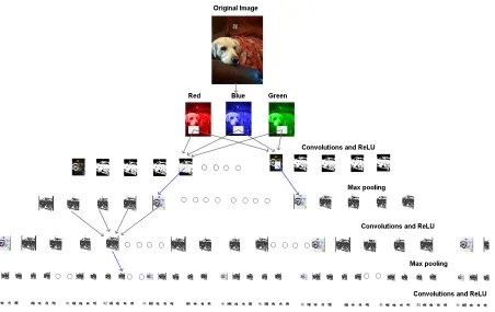
sampled to produce next generation of candidates. [5] . . . 35 3.2 Concept of Convolutional Neural Network depitcts an image of a dog

broken up into RGB (red, green and blue) inputs before feeding it to

the first convolutional layer. Each square box shows a feature map.

Image adapted from [18]. . . 40 3.3 Variational Autoencoder structure showing the parent vectors on top

layer mapped to higher dimensional spaces in encoder f(x). The z layer

provides the probability distribution sampling function, which is

sam-pled by the decoding layers g(x) to yield the output in real dimension

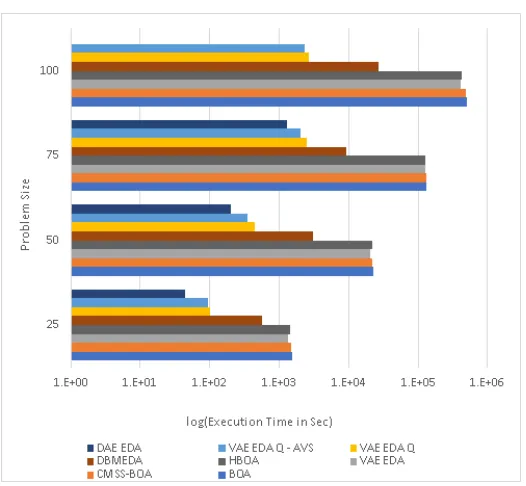
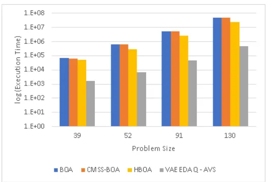
at the bottom layer. . . 44 3.4 Encoding of a Skip layer [22] . . . 48 3.5 Execution time for Trap 5 comparing BOA, HBOA, CMSS-BOA,

VAE-EDA, VAE-EDA-Q, VAE-EDA-Q AVS, DBM-VAE-EDA, and DAE-EDA.

VAE-EDA-Q and VAE-EDA-Q AVS have better performance than

(17)

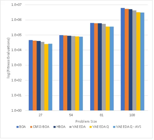
3.6 Number of fitness Evaluations for Trap 5 comparing BOA, HBOA,

CMSS-BOA, VAE-EDA, VAE-EDA-Q, VAE-EDA-Q AVS, DBM-EDA,

and DAE-EDA. VAE-EDA-Q has the lowest number of fitness

evalua-tions compared to all the other algorithms . . . 57 3.7 Execution time for Trap 7 comparing BOA, HBOA, CMSS-BOA,

VAE-EDA, Q AVS, and Q. VAE-EDA and

VAE-EDA-Q perform better than BOA and CMSS-BOA, with VAE-EDA-VAE-EDA-Q

hav-ing the lowest execution time . . . 58 3.8 Number of fitness Evaluations for Trap 7 comparing BOA, HBOA,

CMSS-BOA, EDA, EDA-Q AVS, and EDA-Q.

VAE-EDA and VAE-VAE-EDA-Q perform better than BOA and CMSS-BOA,

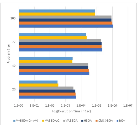
with VAE-EDA-Q having the lowest number of fitness evaluations . . 58 3.9 Execution time for Trap 9 comparing BOA, HBOA, CMSS-BOA,

VAE-EDA, VAE-EDA-Q AVS, and VAE-EDA-Q. VAE-EDA-Q AVS and

VAE-EDA-Q perform better than VAE-EDA, BOA and CMSS-BOA,

with VAE-EDA-Q having the lowest execution time . . . 59 3.10 Number of fitness Evaluations for Trap 9 comparing BOA, HBOA,

CMSS-BOA, EDA, EDA-Q AVS, and EDA-Q.

VAE-EDA-Q and VAE-VAE-EDA-Q AVS perform better than VAE-EDA, BOA

and CMSS-BOA, with VAE-EDA-Q having the lowest number of fitness

evaluations. . . 59 3.11 Execution time for Trap 11 comparing BOA, HBOA, CMSS-BOA, and

VAE-EDA-Q AVS. VAE-EDA-Q AVS has lower execution time

(18)

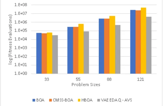
3.12 Number of fitness Evaluations for Trap 11 comparing BOA, HBOA,

CMSS-BOA, and VAE-EDA-Q AVS. VAE-EDA-Q AVS has lower

num-ber of fitness evaluations compared to BOA and CMSS-BOA for all

problem sizes. . . 61 3.13 Execution time for Trap 13 comparing BOA, HBOA, CMSS-BOA,

VAE-EDA, VAE-EDA-Q AVS, and VAE-EDA-Q. VAE-EDA-Q AVS

has lower execution time compared to BOA and CMSS-BOA for all

problem sizes. . . 62 3.14 Number of fitness Evaluations for Trap 13 comparing BOA, HBOA,

CMSS-BOA, and VAE-EDA-Q AVS. VAE-EDA-Q AVS has lower

num-ber of fitness evaluations compared to BOA and CMSS-BOA for all

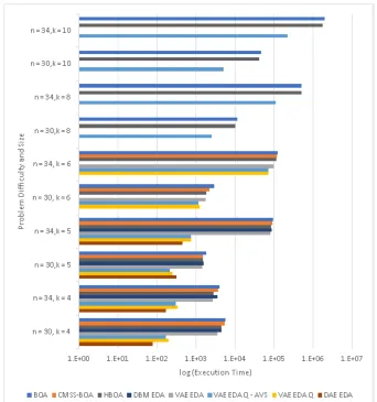
problem sizes. . . 62 3.15 Execution time for NK Landscapes comparing BOA, HBOA,

CMSS-BOA, VAE-EDA, VAE-EDA-Q, VAE-EDA-Q AVS, DBM-EDA, and

DAE-EDA. DAE-EDA has lowest execution time upto k = 5.

VAE-EDA-Q AVS is able to solve K = 8 and K = 10 at better performance

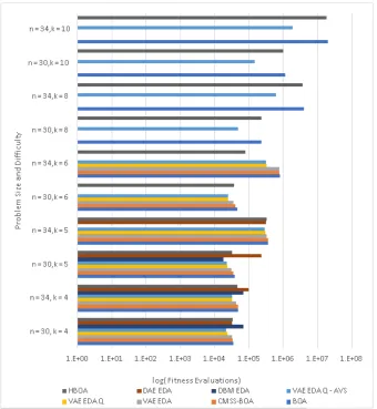
than BOA. . . 64 3.16 Number of fitness evaluations for NK Landscapes comparing BOA,

HBOA, CMSS-BOA, VAE-EDA, VAE-EDA-Q, VAE-EDA-Q AVS,

DBM-EDA, and DAE-EDA. VAE-EDA-Q has lowest number of fitness

eval-uations compared to all other algorithms. VAE-EDA-Q AVS is able to

(19)

4.1 An example of a simple FCM in which activation of foeClose (proximity

to predator) and foeFar (distant predator) is given by fuzzification of

these concepts, depending on the distance of prey from predator. In the

fuzzification process the real value of the sensory concept (say predator

is 5 cells away) is converted to a fuzzy value (say a decimal number from

0 to 1). The speed at which prey evade is given by defuzzificaton of

evasion concept, where the reverse of fuzzification happens - the fuzzy

value is converted to a real scalar value. The L matrix is an nxn matrix

showing influence of one concept on another; where 0 denotes foeClose,

1 denotes foeFar, 2 represents fear and 3 represents evasion. Activation

levels of motor concepts in EcoSim dictate what action an individual

will take next and the defuzzification of the activation level provide the

intensity of the action. For example if evasion concept is activated, the

defuzzification of evasion concept gives the speed of evasion. [41] . . . 92 4.2 Measuring whether statiscally significant differences exist in species

rates, for varying values of reproductive penalty parameter based on

coefficient c. Sensitivity analysis experiments for extinction rate has

same setup. . . 106 4.3 Extinction rates when the coefficient of penalty imposed on female prey

for reproductive failure is varied from 0.5 to 1.5 in steps of 0.25. The

differences observed are not statistically significant. . . 107 4.4 Speciation rates observed are not significant, when the coefficient of

penalty imposed on female prey for reproductive failure is varied from

0.5 to 1.5 in steps of 0.25. The differences observed are not statistically

(20)

4.5 C4.5 model depicting a decision tree to predict speciation levels in Good

genes mating based on threshold values of various parameters. A node

represents a decision variable to predict speciation level (high or low)

at the leaf. A path from various nodes to a leaf represent a conditional

rule, based on the nodes in the path (decision variables). There are two

numbers associated with each leaf node. The first number indicates

the total number of instances reaching that leaf (rule) while the second

number indicates the number of misclassified instances. The leaves of

the branches with maximum number of instances have been underlined

with blue color . . . 113 4.6 C4.5 model depicting a decision tree to predict speciation levels in

ran-dom mating based on threshold values of various parameters. A node

represents a decision variable to predict speciation level (high or low) at

the leaf. A path from various nodes to a leaf represents a conditional

rule, based on the nodes in the path (decision variables). There are

two numbers associated with each leaf node. The first number

indi-cates the total number of instances reaching that leaf (rule) while the

second number indicates the number of misclassified instances. The

leaves of the branches with maximum number of instances have been

underlined with blue color . . . 115 4.7 C4.5 model depicting a decision tree to predict extinction levels in Good

genes mating based on threshold values of various parameters. A node

represents a decision variable to predict extinction levels (high or low)

at the leaf. A path from various nodes to a leaf represents a conditional

rule, based on the nodes in the path (decision variables). There are two

(21)

4.8 C4.5 model depicting a decision tree to predict extinction levels in

ran-dom mating. A node represents a decision variable to predict extinction

levels (high or low) at the leaf. A path from various nodes to a leaf

represents a conditional rule, based on the nodes in the path (decision

variables). There are two numbers associated with each leaf node. . . 117

5.1 An example of a simple FCM in which activation of predClose (proximal

predator) and predFar (distant predator) is given by fuzzification of

these concepts, depending on the distance of prey from predator. In

the fuzzification process, the real value of the sensory concept (consider

a predator 5 cells away) is converted to a fuzzy value (a decimal number

from 0 to 1). The speed at which prey evade is given by defuzzificaton

of the evasion concept, where the reverse of fuzzification happens

-the fuzzy value is converted to a real scalar value. The L matrix is

an nxn matrix showing the influence of one concept upon another;

where 0 denotes predClose, 1 denotes predFar, 2 represents fear, and

3 represents evasion. Activation levels of motor concepts in EcoSim

dictate choice of action for an individual and the defuzzification of the

activation level provides the intensity of the action. For example, if the

evasion concept is activated, the defuzzification of the evasion concept

gives the speed of evasion. [26] . . . 139 5.2 FCM of a typical prey individual. The left column of nodes contains

the sensory concepts; the middle column of nodes contains the internal

concepts, and the right column of nodes contain the motor concepts.

The red edges denote a negative edge and a blue line denotes a positive

(22)

5.3 An illustration of Communication-related to Danger and Safety shows

the sharing of fear between two individuals near one another. . . 141 5.4 Communication of Fear from Signaler to Receiver. Receiver prey

re-ceived the extra information related to fear, even when the receiver is

unable to sense a predator directly due to a greater distance . . . 142 5.5 Comparing Search Food Ratio between Communication and Non-Communication

Runs . . . 148 5.6 Comparing Search Food Ratio between Communication and Non-Communication

Runs . . . 150 5.7 Number of individuals using links from Communication nodes to other

nodes for Run 8 at 34000th timestep. . . 151 5.8 Individual run impacts of Communicated Danger and Communicated

Safety on Search Food Node at 34000th timestep. . . 153 5.9 FCM Analyzer showing the FCM network of one prey individual and

the connections from Communication Node to various internal nodes

and finally stopping at Search Food.. . . 154 5.10 FCM Analyzer: Effect of varying CommDanger and CommSafety on

(23)

Chapter 1 Introduction

The standard process of study within behavioral ecology is to first observe and inter-pret animal behavior and then form subsequent testable hypotheses [1]. Behavioral ecology, as a subset of all biological disciplines, additionally pays distinct considera-tion to interacconsidera-tions between organisms and the environment [2]. As animal behaviors and ecosystems, in addition to their inter-lying interactions, have the propensity to become exponentially complex, a bottom-up approach of study based on individual traits and behaviors is essential [3]. Individual based modeling facilitates the intri-cate study of discrete organisms as well as their involvement with other organisms and environmental conditions, such as food and predation. Through the creation of an artificial ecosystem, an entire set of interactions gives rise to high-level phenomena that emerge generating the same patterns observed in nature. Speciation, extinc-tion, population migraextinc-tion, and the shape of spatial distribution of individuals are all observable events within artificial ecosystems [4].

(24)

ecology, mathematics, and computer science [5]. Within ecological modeling, artifi-cial ecosystems offer benefits distinct from field studies as they illuminate large-scale views of evolution of systems; this enables a deep understanding of theoretical con-cepts concerning evolutionary process, speciation, and extinction [6]. In this respect, ecosystem simulations could also provide a vast amount of data related to each partic-ular individual. Such insights may be difficult to measure or even infeasible in nature and, thus, the generation of this raw multidimensional data can be invaluable for use in analysis. Data analysis involves collecting, processing, cleaning, transforming, and modeling data in order to produce useful knowledge from which conclusions can be drawn [7], [8].

Machine learning, an approach of data analysis, could be used to extract useful knowledge from large datasets and propose insights. By learning from raw input data, machine learning could also aid in the decision making process [9]. Machine learning methods include regression, classification, feature selection, and rule extrac-tion. Presence of irrelevant features (containing irrelevant, superfluous, and redundant information) affects the reliability and interpretability of knowledge processed by ma-chine learning methods [10]. A class of algorithms known as feature selection aims to ameliorate this issue by identifying and removing datasets of irrelevant features prior to the construction of the predictive model.

(25)

this model determines the suitability of the feature subset. Therefore, the search is wrapped around the classification model in the search of the feature space for the optimal subset.

(26)

Within biological literature, the distinction between sexual selection and pan-mixia (random mating) is undisputed, yet the implications of sexual selection remain a subject of discussion. Demonstration of the presence of panmixia is presented by a number of studies, including [21]. However, the relationship between random mating and speciation and extinction rates is not universally understood based upon exist-ing empirical study alone. Further, empirically based dialogue within the concept of sexual selection, specifically, also lacks concordance. Authors in [22] propose sexual selection to involve variance due to mating success, and natural selection to involve variance with respect to other aspects of fitness. And while the authors of [22] define sexual selection as intra-specific reproductive competition, they also admit it to be a poorly understood concept. Within sexual selection, the concept known as the good genes hypothesis is another fundament that remains open to debate. This concept is based upon the assumption that females who select males with phenotypic traits pre-sumed to manifest good genes will produce fit offspring [23]. While the meta-analysis performed by [23] revealed a correlation between male secondary traits that attract females during mating and offspring survival, authors in [24] determined the role of male secondary traits to be minor in the selection for good genes within Pronghorn.

(27)

Furthermore, the data garnered from our study can be translated to valuable insight reaching far beyond the original empirical queries.

The subject of behavioral influence of animal communication displays discordance similar to that of sexual selection. Evidence exists to support that communication influences behavior, as described by [26] in his study of the influence of honey bee waggle dances upon foraging behavior. However disagreement exists over the direction to which the influence is an effector (increase versus decrease). Within the scope of foraging behavior, there is a high level of empirical corroboration for predator alarm cues and presence of predation decreasing foraging behavior in prey, with specific cases presented in the studies of hard clams, coral reef fish, termites, and crabs [27], [28], [29], [30]. However, ample opposition exists in support of a gradual, long run increase in foraging behavior due to sustained predation and communication of alarm cues – this is known as the predation risk allocation hypothesis. This view employs a cost-benefit analysis to reason that the cost of vulnerability to predation is outweighed by the benefits of acquiring food necessary for survival [31]. Additional corroboration of this theory is presented by a number of studies including [32], [33], [34]. Despite this evidence, authors in [35] and [36] have expressed skepticism.

(28)

Bibliography

[1] Anil K Seth. The ecology of action selection: Insights from artificial life. Philosophical Transactions of the Royal Society B: Biological Sciences, 362(1485):1545–1558, 2007.

[2] John R Krebs and Nicholas B Davies. Behavioural ecology: an evolutionary

approach. John Wiley & Sons, 2009.

[3] Morteza Mahayekhi, Abbas Golestani, Yasaman Farahani, and Robin Gras. n Enhanced Artificial Ecosystem: Investigating Emergence of Ecological Niches. In

Artificial Life Conference Proceedings 14, pages 693–700. MIT Press, 2014.

[4] Morteza Mashayekhi. Individual-Based Modeling and Data Analysis of Ecological Systems Using Machine Learning Techniques. 2015.

[5] Carlo Ricotta. From theoretical ecology to statistical physics and back: self-similar landscape metrics as a synthesis of ecological diversity and geometrical complexity. Ecological Modelling, 125(2-3):245–253, 2000.

[6] Didier Devaurs and Robin Gras. Species abundance patterns in an ecosystem simulation studied through Fisher’s logseries. Simulation Modelling Practice and

Theory, 18(1):100–123, 2010.

[7] Geoffrey Keppel and Sheldon Zedeck.Data analysis for research designs. Macmil-lan, 1989.

[8] Cathy O’Neil and Rachel Schutt. Doing data science: Straight talk from the

frontline. " O’Reilly Media, Inc.", 2013.

(29)

[10] Mark A Hall and Lloyd A Smith. Practical feature subset selection for machine learning. 1998.

[11] Yvan Saeys, Iñaki Inza, and Pedro Larrañaga. A review of feature selection techniques in bioinformatics. bioinformatics, 23(19):2507–2517, 2007.

[12] Shumeet Baluja. Population-based incremental learning. a method for integrating genetic search based function optimization and competitive learning. Technical report, Carnegie-Mellon Univ Pittsburgh Pa Dept Of Computer Science, 1994.

[13] Heinz Mühlenbein and Gerhard Paass. From recombination of genes to the es-timation of distributions I. Binary parameters. In International conference on

parallel problem solving from nature, pages 178–187. Springer, 1996.

[14] Pedro Larrañaga and Jose A Lozano. Estimation of distribution algorithms: A

new tool for evolutionary computation, volume 2. Springer Science & Business

Media, 2001.

[15] Iñaki Inza, Pedro Larrañaga, Ramón Etxeberria, and Basilio Sierra. Feature subset selection by Bayesian network-based optimization. Artificial intelligence, 123(1-2):157–184, 2000.

[16] Marwa Khater and Robin Gras. Adaptation and genomic evolution in ecosim. InInternational Conference on Simulation of Adaptive Behavior, pages 219–229. Springer, 2012.

[17] Elham Salehi and Robin Gras. Efficient EDA for large opimization problems via constraining the search space of models. In Proceedings of the 13th annual

conference companion on Genetic and evolutionary computation, pages 73–74.

(30)

[18] Diederik P Kingma and Max Welling. Auto-encoding variational bayes. arXiv

preprint arXiv:1312.6114, 2013.

[19] Danilo Jimenez Rezende, Shakir Mohamed, and Daan Wierstra. Stochastic back-propagation and approximate inference in deep generative models.arXiv preprint

arXiv:1401.4082, 2014.

[20] Robin Gras, Didier Devaurs, Adrianna Wozniak, and Adam Aspinall. An individual-based evolving predator-prey ecosystem simulation using a fuzzy cog-nitive map as the behavior model. Artificial life, 15(4):423–463, 2009.

[21] Johan Dannewitz, Gregory E Maes, Leif Johansson, Håkan Wickström, Filip AM Volckaert, and Torbjörn Järvi. Panmixia in the European eel: a matter of time. . . . Proceedings of the Royal Society B: Biological Sciences, 272(1568):1129– 1137, 2005.

[22] David J Hosken and Clarissa M House. Sexual selection. Current Biology, 21(2):R62–R65, 2011.

[23] Anders Pape MÖller and Rauno V Alatalo. Good-genes effects in sexual selec-tion. Proceedings of the Royal Society of London. Series B: Biological Sciences, 266(1414):85–91, 1999.

[24] John A Byers and Lisette Waits. Good genes sexual selection in nature.

Pro-ceedings of the National Academy of Sciences, 103(44):16343–16345, 2006.

[25] Sourodeep Bhattacharjee, Brian MacPherson, and Robin Gras. A comparison of sexual selection versus random selection with respect to extinction and spe-ciation rates using individual based modeling and machine learning. Ecological

(31)

[26] Karl Von Frisch. The dance language and orientation of bees. 1967.

[27] Delbert L Smee and Marc J Weissburg. Hard clams (Mercenaria mercenaria) evaluate predation risk using chemical signals from predators and injured con-specifics. Journal of chemical ecology, 32(3):605–619, 2006.

[28] Matthew D Mitchell, Peter F Cowman, and Mark I McCormick. Chemical alarm cues are conserved within the coral reef fish family Pomacentridae. Plos one, 7(10):e47428, 2012.

[29] R Inta, TA Evans, and JCS Lai. Effect of vibratory soldier alarm signals on the foraging behavior of subterranean termites (Isoptera: Rhinotermitidae). Journal

of economic entomology, 102(1):121–126, 2009.

[30] A Randall Hughes, David A Mann, and David L Kimbro. Predatory fish sounds can alter crab foraging behaviour and influence bivalve abundance. Proceedings

of the Royal Society B: Biological Sciences, 281(1788):20140715, 2014.

[31] Steven L Lima and Peter A Bednekoff. Temporal variation in danger drives antipredator behavior: the predation risk allocation hypothesis. The American

Naturalist, 153(6):649–659, 1999.

[32] Andrew Sih and Thomas M McCarthy. Prey responses to pulses of risk and safety: testing the risk allocation hypothesis. Animal Behaviour, 63(3):437–443, 2002.

(32)

[34] Stefanie Slos and Robby Stoks. Behavioural correlations may cause partial sup-port for the risk allocation hypothesis in damselfly larvae. Ethology, 112(2):143– 151, 2006.

[35] Maud CO Ferrari, Andrew Sih, and Douglas P Chivers. The paradox of risk allocation: a review and prospectus. Animal Behaviour, 78(3):579–585, 2009.

[36] Guy Beauchamp and Graeme D Ruxton. A reassessment of the predation risk allocation hypothesis: a comment on Lima and Bednekoff. The American

(33)

Chapter 2 Background

2.1 Individual Based Modeling

2.1.1 Need for Individual Based Modeling

Models, in general, are simplified representations of real systems and universally share the challenge of proving their predictive capabilities [1]. Ecological models, however, have the unique requirement of depicting relevant spatial and temporal scales in tan-dem with a multitude of processes representative of the system observed [2]. Eco-logical models support environmental decision making in ways that corresponding experiments cannot as conclusions drawn from descriptive studies have the potential of failing to fully represent processes [3]. While the study of ecology involves entire populations, communities, and ecosystems, the properties of the system are princi-pally determined by the properties and behavior of the individuals from which they are composed. Therefore, individuals are the foundation of ecological models [4].

(34)

of matter. This illuminates a key difference – individual organisms have biotic proper-ties that atoms lack. The principles of life cycles, growth, development, reproduction, and death are conserved throughout ecological systems despite the transient nature of the individuals to which they belong. Additionally, individuals modify their environ-ments through interaction with resources; even within the same species, differences allow individuals to modify the environment in distinctive ways. Most important, though, is the concept of adaptation wherein individuals are able to grow, mature, obtain resources, reproduce, and interact depending upon intrinsic and extrinsic fac-tors [4]. This notion highlights the difference between atomic theory and ecology – individual organisms are adaptive because their response to biotic and abiotic factors determines their ability to pass their genes on to future generations (fitness). Fur-thermore, fitness-seeking adaptation does not occur to advance the population as a whole; behavioral adaptation occurs at the level of the individual.

2.1.2 What is Individual Based Modeling?

Individual based models are capable of handling the high degree of complexity in the representation of individuals and interactions among individuals. This approach (also known as agent based models) is described to simulate populations and systems with respect to each individual organism [5]. Individuals have their own set of state vari-ables, which include spatial location and physiological or behavioral traits. Attributes such as growth, habitat selection, foraging, reproduction, and dispersal are able to differ among individuals and change over time [6].

(35)

a bottom-up approach where interactions among discrete, autonomous individuals, as well as among their abiotic environments, drive the population level behaviors [8] and [9]. These interactions are the foundation of emergent properties like species distribution at the population and ecosystem levels [7]. By employing discrete units, the incorporation of individual level mechanisms can be represented. This is in direct contrast to traditional models where complexity and interactions cannot be repre-sented to this degree. IBM makes possible the examination of variation of individuals at life cycle stages, variation among individuals, local interactions among individuals, and adaptive behaviors such as energy budgets and physiology [6]. Authors in [7] sug-gest that the distinguishing characteristics amount to four keys: degree of complexity of individual life cycles, variation of resources used, quantities measured in discrete numbers versus real numbers, and variation among individuals of the same age.

(36)

IBMs as the unique experiences of each individual, in addition to variation caused by ontogenetic changes, can be used to determine trajectory. Using plants as an example, it is possible to illustrate how the inclusion of details such as soil, water, nutrients, and light gives rise to an incredibly more precise history. Cognitive variability shares a similar foundation with phenotypic variability within individual based modeling – experience and learning are derived from individual experiences. Memories of past experiences are considered to be an internal state and give rise to learning, which can arise from the environment of another organism. Genetic variability and evolu-tion studies have classically focused on the individual. Mutaevolu-tions, genetic drift, and founder effects are examples of evolutionary genetic concepts that involve a small number of individuals yet create a profound effect. IBM also uses an individualistic foundation, which makes the concept of stochasticity significant. IBMs have a higher degree of flexibility than classical models, which allows for the analogous representa-tion of true popularepresenta-tion change.

2.1.3 Harnessing the power of IBM for Ecological and

Evo-lutionary Processes

(37)

paradigmatic IBMs [8].

i Local interactions and movement - The examination of movement through space entails modeling a vast grouping of detailed active movement behaviors from local interaction with animals and landscapes to development of home ranges.

ii Formation of patterns among individuals - Formation of patterns among indi-viduals describes the study of how social forces, environmental factors, and individual decisions give rise to swarms or other aggregations.

iii Interactions of exploitative species - When considering exploitative species, spatial movement patterns have been shown to radically affect the stability of the interaction through the diffusion and mixing of populations in predator-prey and host-parasitoid interactions.

iv Community dynamics and local competition - When examining sessile organ-isms, focus on emergent phenomena and community dynamics are of great interest and are studied using grid cells or continuum models. Competition-colonization trade off, effects of conspecific density, and niche differences are all able to interact in spatial context to illustrate factors that control species richness and diversity.

(38)

vi Evolutionary process - Evolutionary process modeling seeks to answer a mul-titude of queries, which range from comparisons of trait values to genetic algorithms examining optimal traits for foraging, avoidance of predators, reproduction, and dis-persal. While they do not replicate mechanisms of evolution, these models do conserve genetic diversity and have even predicted settings in which polymorphisms could be maintained within populations.

Through a radical departure from classical mathematical approaches to ecological theory, IBM has established a new philosophical paradigm. By requiring the inclusion of individual detail into models, the term IBM is considered tantamount to an explicit examination of individuals and their complex responses to their environments [8]. The rule-based simulations employed by IBM are optimal for responses such as phenotypi-cal change and learning than are their mathematiphenotypi-cal model counterparts. Population and community level behaviors arise from adaptive behaviors of individuals. Future developments will focus on further sophistication of representations of internal states and increased autonomy. This will shed light on the decisions of individuals and on behaviors such as mating. Pattern oriented modeling will allow the comparison of model behavior to natural systems [13]. Authors in [9] uphold that a formally docu-mented model is sufficient in terms of rigor and that mathematical notation is not a requisite. The future development of individual based modeling will play a great role in paradigmatic ecology and may provide understanding for the basis of evolution [10].

Bibliography

[1] Edward J Rykiel Jr. Modeling agroecosystems: Lessons from ecology.Agricultural

(39)

[2] Amelie Schmolke, Pernille Thorbek, Donald L DeAngelis, and Volker Grimm. Ecological models supporting environmental decision making: a strategy for the future. Trends in ecology & evolution, 25(8):479–486, 2010.

[3] Jacqueline Augusiak, Paul J Van den Brink, and Volker Grimm. Merging valida-tion and evaluavalida-tion of ecological models to ‘evaludavalida-tion’: a review of terminology and a practical approach. Ecological Modelling, 280:117–128, 2014.

[4] Volker Grimm and Steven F Railsback. Individual-based modeling and ecology, volume 8. Princeton university press, 2013.

[5] H Van Dyke Parunak, Robert Savit, and Rick L Riolo. Agent-based modeling vs. equation-based modeling: A case study and users’ guide. In International

Workshop on Multi-Agent Systems and Agent-Based Simulation, pages 10–25.

Springer, 1998.

[6] Donald L DeAngelis and Volker Grimm. Individual-based models in ecology after four decades. F1000prime reports, 6, 2014.

[7] Brian MacPherson and Robin Gras. Individual-based ecological models: Adjunc-tive tools or experimental systems? Ecological Modelling, 323:106–114, 2016.

[8] Donald L DeAngelis and Wolf M Mooij. Individual-based modeling of ecological and evolutionary processes. Annu. Rev. Ecol. Evol. Syst., 36:147–168, 2005.

[9] V Grimm and SF Railsback. Individual-based modeling and ecology, 480 pp, 2005.

(40)

[11] Adam Lomnicki. Population ecology of individuals. Princeton University Press, 1988.

[12] Janusz Uchmański. Differentiation and frequency distributions of body weights in plants and animals.Philosophical Transactions of the Royal Society of London.

B, Biological Sciences, 310(1142):1–75, 1985.

[13] Volker Grimm, Karin Frank, Florian Jeltsch, Roland Brandl, Janusz Uchmański, and Christian Wissel. Pattern-oriented modelling in population ecology. Science

(41)

2.2 Estimation of Distribution Algorithms:

Ma-chine Learning Approaches

2.2.1 Introduction to Machine Learning Based EDA

Estimation of Distribution Algorithms (EDA) [1], [2] are algorithms that employ meta-heuristics to aid in combinatorial and continuous non-linear optimization [3]. Within EDA, an efficient probabilistic model guides the search towards solutions of higher fitness, compared to solutions of the previous generation. The model is generated by encoding the probability distribution of admissible solutions based on their fitness values [4]. EDA performs a random sampling of the probabilistic model to yield new solutions representative of the population as a whole, while maintaining a similar or desirably better solution quality than the present solutions of the population. In order to discover the optimal solution, EDA initiates a population of uniformly and randomly generated candidate solutions. This population of candidate solutions is iteratively improved upon over consecutive generations. EDA estimates the possibil-ity of a candidate to lead to an optimal offspring over subsequent generations while also discerning the hidden interdependencies between the constituent features in the candidate.

(42)

model of the population. These models solve problems composed of subproblems of overlapping variables that cannot be decomposed into independent subproblems due to inter-dependency. This method facilitates the solving of very complex problems; however, estimating the model from a population can be very computationally de-manding. The production of a probabilistic model that is both flexible and efficient in terms of estimation and sampling is of prime importance. Parallel research in the field of Machine Learning algorithms shares the same focus, for example unsupervised machine learning algorithms for generative neural networks [3]. These algorithms are able to accept high dimensional data as input, from which they are able to learn complex patterns. Generative neural networks produce models from a population of samples in an unsupervised manner and are capable of generating from them com-pletely new solutions having the same likelihood distribution. This makes them very useful for EDA applications as they perform better exploration of the search space while using less time and computational resources. These generative neural network models can be stacked upon each other in layers and provide building blocks for use in deep learning.

2.2.2 Restricted Boltzmann Machine EDA

(43)

evalua-tion is required for RBM-EDA than BOA, which would indicate that the populaevalua-tion model of RBM-EDA was less accurate than the statistical model of BOA. However, the authors also stipulated that the quality of the model was compensated for by the shorter model building time for RBM-EDA. They also found that the CPU time for RBM-EDA grew at a slower rate than BOA with an increase in problem sizes; and for difficult problems, the performance of RBM-EDA was similar or superior to BOA.

2.2.3 Denoising Autoencoder EDA

Autoencoders [8–10] are neural networks that learn an abstract representation of the input through an encoder model and later performing a reconstruction step using a decoder. This process converts the representation to an output that approximates the distribution of training examples. Autoencoders have been utilized as generative modeling techniques in dimensionality reduction and for feature learning applications [11].

(44)

a reduced optimization score. In some cases, DAE-EDA was able to reach quicker con-vergence in term of number of fitness evaluations, but in most other cases it required larger population sizes to achieve guaranteed convergence.

2.2.4 Deep Boltzmann Machines EDA

Deep Boltzmann Machines (DBM) [15] are deep neural networks consisting of multiple layers of hidden neurons, and can thus be used to capture the model of the population at increasing layers of abstraction. Each hidden layer provides one additional layer of abstraction capable of representing patterns or features in the data. Authors in [16] used DBM with EDA based on the promise shown by the results in RBM-EDA and on the success of deep learning models. Following similar experimental benchmarks as in RBM, the authors found that while DBM-EDA was computationally less expensive than BOA, the quality of the solutions was inferior to BOA in cases of multi modal problems beyond trap-5. Furthermore, the authors specified that given the efforts needed to train the multi-layer DBM-EDA, it was not feasible to be used in a noisy training set. DBM-EDA was not able to find the global optimum in complex problems when allotted the same population size as BOA.

2.2.5 Generative Adversarial Network EDA

(45)

of the generator is to produce new solutions that very closely reflect the distribution of the population such that the discriminator cannot detect the new solution as a synthesized outlier. Authors in [17] tested GAN-EDA on one-max problems, concate-nated trap functions, and NK Landscapes. GAN EDA displayed lower performance than both DAE-EDA and BOA for the test problems presented and in most cases was unable to find the global optimum.

2.2.6 Variational Autoencoder EDA

(46)

The authors proposed two extensions of VAE-EDA. The first extension, named Extended VAE (E-VAE), contained a second decoder along with the standard encoder-decoder. The second decoder was used to learn to predict the fitness value of the output. The second extension proposed by the authors in [22] is titled Conditioned, Extended VAE (CE-VAE) and proposed to use the predictor to explicitly sample the solutions with best-predicted fitness. In this extension, the predictor accepted the output of the encoder (same as the decoder that outputs the off-spring), and the predictor and decoder were trained simultaneously. This predictor demonstrated efficacy as a regularizer component for the latent representation and also demonstrated potential to be used as a surrogate fitness function in situations where the actual fitness computation required a great amount of time. Substituting the surrogate fitness function was found to improve the overall performance of the algorithm in cases such as this. This method, however, was not tested on any benchmark problems or compared to any state-of-the-art algorithms. Authors in [22] merely compared the relative performance of three methods on a simplified protein folding problem that had a single objective.

Bibliography

(47)

[3] Malte Probst, Franz Rothlauf, and Jörn Grahl. Scalability of using Restricted Boltzmann Machines for combinatorial optimization. European Journal of

Oper-ational Research, 256(2):368–383, 2017.

[4] Martin Pelikan, Mark W Hauschild, and Fernando G Lobo. Estimation of dis-tribution algorithms. InSpringer Handbook of Computational Intelligence, pages 899–928. Springer, 2015.

[5] Martin Pelikan, David E Goldberg, and Erick Cantu-Paz. Linkage problem, distribution estimation, and Bayesian networks. Evolutionary computation, 8(3):311–340, 2000.

[6] Martin Pelikan, David E Goldberg, and Erick Cantú-Paz. BOA: The Bayesian optimization algorithm. In Proceedings of the 1st Annual Conference on

Ge-netic and Evolutionary Computation-Volume 1, pages 525–532. Morgan

Kauf-mann Publishers Inc., 1999.

[7] Paul Smolensky. Parallel distributed processing: Explorations in the microstruc-ture of cognition, vol. 1. chapter Information Processing in Dynamical Systems: Foundations of Harmony Theory.MIT Press, Cambridge, MA, USA, 15:18, 1986.

[8] Geoffrey E Hinton and Ruslan R Salakhutdinov. Reducing the dimensionality of data with neural networks. science, 313(5786):504–507, 2006.

[9] Y-lan Boureau, Yann L Cun, et al. Sparse feature learning for deep belief net-works. In Advances in neural information processing systems, pages 1185–1192, 2008.

[10] Yoshua Bengio et al. Learning deep architectures for AI.Foundations and trends®

(48)

[11] Yoshua Bengio, Aaron Courville, and Pascal Vincent. Representation learning: A review and new perspectives.IEEE transactions on pattern analysis and machine

intelligence, 35(8):1798–1828, 2013.

[12] Yoshua Bengio, Li Yao, Guillaume Alain, and Pascal Vincent. Generalized de-noising auto-encoders as generative models. InAdvances in Neural Information

Processing Systems, pages 899–907, 2013.

[13] Pascal Vincent, Hugo Larochelle, Yoshua Bengio, and Pierre-Antoine Manzagol. Extracting and composing robust features with denoising autoencoders. In

Pro-ceedings of the 25th international conference on Machine learning, pages 1096–

1103. ACM, 2008.

[14] Malte Probst. Denoising autoencoders for fast combinatorial black box optimiza-tion. InProceedings of the Companion Publication of the 2015 Annual Conference

on Genetic and Evolutionary Computation, pages 1459–1460. ACM, 2015.

[15] Ruslan Salakhutdinov and Geoffrey Hinton. Deep Boltzmann Machines. In David van Dyk and Max Welling, editors,Proceedings of the Twelth International

Con-ference on Artificial Intelligence and Statistics, volume 5 of Proceedings of

Ma-chine Learning Research, pages 448–455, Hilton Clearwater Beach Resort,

Clear-water Beach, Florida USA, 2009. PMLR.

[16] Malte Probst and Franz Rothlauf. Deep boltzmann machines in estima-tion of distribuestima-tion algorithms for combinatorial optimizaestima-tion. arXiv preprint

arXiv:1509.06535, 2015.

(49)

[18] Diederik P Kingma and Max Welling. Auto-encoding variational bayes. arXiv

preprint arXiv:1312.6114, 2013.

[19] Danilo Jimenez Rezende, Shakir Mohamed, and Daan Wierstra. Stochastic back-propagation and approximate inference in deep generative models.arXiv preprint

arXiv:1401.4082, 2014.

[20] Carl Doersch. Tutorial on variational autoencoders. arXiv preprint

arXiv:1606.05908, 2016.

[21] Jinwon An and Sungzoon Cho. Variational autoencoder based anomaly detection using reconstruction probability. Special Lecture on IE, 2:1–18, 2015.

[22] Unai Garciarena, Roberto Santana, and Alexander Mendiburu. Expanding vari-ational autoencoders for learning and exploiting latent representations in search distributions. InProceedings of the Genetic and Evolutionary Computation

(50)

2.3 Wrapper Based Feature Selection and EDA

Approaches

When machine learning algorithms are applied on high dimensional data, an issue known as curse of dimensionality arises, where as the number of dimension increases, the volume of the data space increases and the amount of data available becomes sparser [1]. Sparse data adverse affects the efficacy and the solution quality of several machine learning algorithms [2] for example for classification models that work on grouping instances based on their similarities to come up with a model, struggle to make such groupings when due to extraneous features they mind most instances to be dissimilar. Sometimes the presence of a large number of features causes learning models to overfit the training data which degrades the solutions given by the model when tested on novel data. Not only that, working with high dimensional data in-creases memory requirements and puts a higher demand on computational costs for machine learning algorithms [2].

A class of machine learning algorithms exist to tackle the issues arising from high dimensional data. These algorithms are known as Dimensionality reduction algo-rithms and are categorized into two groups: Feature Selection and Feature Extrac-tion. In Feature Extraction, subsets of higher dimensional data are combined linearly or non-linearly and the output is mapped to a new feature space. The features in the new feature space thus created have lower number of dimensions than the original feature space. On the other hand, feature selection directly choses a subset of features from the original feature space to lower the dimensionality [3] [4].

(51)

ex-traction produces high level features by combining features from the original feature space. These high-level features are making it difficult to interpret the resulting model built from these high-level features. Hence, in many cases feature selection becomes a preferred choice as it retains the relevant original features and only removes the unnecessary features, thereby maintaining the ease of interpretation of the models generated from the subset [2]. Even in cases where the original number of features are not too high, feature selection is often employed to reduce computational costs and to improve model quality. Moreover, real-world data often contains a lot of noisy fea-tures that are irrelevant and sometimes redundant. Removal of such feafea-tures improve the performance of machine learning algorithms while improving computational effi-ciency. In the context of this body of research, we will focus our discussion on feature selection methods.

Features selection techniques are classified into three categories based on the level of coupling with other machine learning algorithms (such as classification algorithms). Thus, depending on the method the feature selection search is performed along with the construction of classification model, the feature selection algorithms can be clas-sified as: Filter methods, Wrapper methods and Embedded Methods [5].

(52)

spe-cific subset of features produced is evaluated by using the feature subset to train and test a specific classification algorithm and model. Hence this method is very tightly coupled with the specific problem domain and classification method employed. A major advantage of wrapper method is that they take into account the interaction between model search and feature subset search and can also discover feature depen-dencies. Disadvantages of wrapper method is that they tend to overfit the data and are computationally expensive.

Estimation of Distribution Algorithms (EDA) [6], [7] have been used for feature subset search in wrapper methods in previous research. In [8] the authors proposed a novel algorithm - Feature Subset Selection by Estimation of Bayesian Network Algo-rithm (FSS - EBNA) which uses Estimation of Bayesian Network AlgoAlgo-rithm [9] which follows EDA paradigm for feature subset selection. EDAs evolves the population by altering probability distribution of the highest fitness candidates in the population of candidates in each iteration of the search. In EBNA, the evolution of the model is performed by a Bayesian network working in tandem with a local search method. Authors claimed FSS-EBNA to be a computationally efficient wrapper method that can be successfully applied to any problem where specific domain knowledge is not available and where number of samples available is very low.

In [10] the authors used wrapper methods with EDAs to classify cancerous genes in gene expression datasets. They successfully used naïve Bayes classifier with EDA as a wrapper, to considerably reduce the number genes in their classification model, leading to a concise model that is easy to interpret which was a critical requirement for their problem. EDAs, specifically Population based Incremental Learning [11] along COMIT which is a dependency tree based EDA, were used as wrappers in [12] for predicting survival rates of cirrhotic patients.

(53)

from EcoSim, an artificial ecosystem simulator [14]. One of the objectives of this study was to discover the genes that have a stronger influence on fitness of individu-als. In order to achieve this, the authors wrapped CMSS-BOA [15] for feature search on to Random Forests [16] for classification. CMSS-BOA does not restrict a fixed upper bound on the number of variables on which another variable can have some dependency with, leading to discovery of intricate and highly relevant interdependen-cies between variables. Each subset of interdependent variables is encoded as a string of bits. The subset that maximizes the Area under ROC curve (AUC) obtained by Bayesian network classifier is selected.

In conclusion, feature selection is an effective and efficient tool to address the prob-lems associated with high dimensional datasets leading to concise and interpretable machine learning models which can be built in reasonable amount of computational time and resources. Wrapper methods integrate the feature subset search with clas-sifier model search leading to selection of subset of features that are guaranteed to result in better classification models. Estimation of Distribution algorithms being computationally efficient tools for continuous and non-linear combinatorial optimiza-tions have proven to be a good choice for use as a wrapper method in feature subset search and selection in previous research.

Bibliography

[1] Jerome Friedman, Trevor Hastie, and Robert Tibshirani. The elements of

statis-tical learning, volume 1. Springer series in statistics New York, 2001.

[2] Jundong Li, Kewei Cheng, Suhang Wang, Fred Morstatter, Robert P Trevino, Jiliang Tang, and Huan Liu. Feature selection: A data perspective. ACM

(54)

[3] Isabelle Guyon, Steve Gunn, Masoud Nikravesh, and Lofti A Zadeh. Feature

extraction: foundations and applications, volume 207. Springer, 2008.

[4] Huan Liu and Hiroshi Motoda. Computational methods of feature selection. CRC Press, 2007.

[5] Yvan Saeys, Iñaki Inza, and Pedro Larrañaga. A review of feature selection techniques in bioinformatics. bioinformatics, 23(19):2507–2517, 2007.

Media, 2001.

[8] Iñaki Inza, Pedro Larrañaga, Ramón Etxeberria, and Basilio Sierra. Feature subset selection by Bayesian network-based optimization. Artificial intelligence, 123(1-2):157–184, 2000.

[9] Ramon Etxeberria. Global optimization using Bayesian networks. In Proc. 2nd

Symposium on Artificial Intelligence (CIMAF-99), 1999.

[10] Rosa Blanco, Pedro Larrañaga, Iñaki Inza, and Basilio Sierra. Gene selection for cancer classification using wrapper approaches. International Journal of Pattern

Recognition and Artificial Intelligence, 18(08):1373–1390, 2004.

(55)

[12] Iñaki Inza, Marisa Merino, Pedro Larrañaga, Jorge Quiroga, Basilio Sierra, and Marcos Girala. Feature subset selection by genetic algorithms and estimation of distribution algorithms: A case study in the survival of cirrhotic patients treated with TIPS. Artificial Intelligence in Medicine, 23(2):187–205, 2001.

[13] Marwa Khater and Robin Gras. Adaptation and genomic evolution in ecosim. InInternational Conference on Simulation of Adaptive Behavior, pages 219–229. Springer, 2012.

[14] Robin Gras, Didier Devaurs, Adrianna Wozniak, and Adam Aspinall. An individual-based evolving predator-prey ecosystem simulation using a fuzzy cog-nitive map as the behavior model. Artificial life, 15(4):423–463, 2009.

[15] Elham Salehi and Robin Gras. Efficient EDA for large opimization problems via constraining the search space of models. In Proceedings of the 13th annual

conference companion on Genetic and evolutionary computation, pages 73–74.

ACM, 2011.

(56)

Chapter 3 Estimation of Distribution using

Population Queue based

Variational Autoencoders

3.1 Introduction

(57)

Figure 3.1: EDA Procedure: The initial population is assigned a fitness value by application of a fitness function on the candidate, and a selection step is applied to pick the fittest candidates out of the parent pool. A simple probabilistic model is created from the fittest parents which is then sampled to produce next generation of candidates. [5]

potentially closer to the global optima.

In recent studies, Machine Learning techniques have been employed to build pop-ulation models with considerable success. Restricted Boltzmann Machine (RBM) [6] comprised of a stochastic neural network was used as population model [7] and dis-played a considerably less computational time requirement than BOA. In another work, the authors implemented Deep Boltzmann Machine (DBM) to generate the next batches of solutions [8]. Autoencoders [9,10] have also been used to model the population of promising solutions [11].

(58)

premature convergence to a sub-optimal region of the solution-space by learning the model on a set of candidate solutions generated on a range of previous generations (modeled as a queue of populations) of the VAE-EDA process. Another extension proposed in this work uses Adaptive Variance Scaling (AVS) [14] to dynamically con-trol the rate of exploration of the latent space by using a coefficient multiplied to the variance of sampling.

The success of machine learning heavily relies on human machine learning experts who are responsible for feature selection, workflow design, selection and design of machine learning models, and hyper-parameters. There is a growing demand for self-contained machine learning methods that can be used within a variety of domains without the necessity of the involvement of machine learning human experts. To this effect, [15] a new field of research targeting progressive automation of machine learning, known as AutoML, is being pursued. The term AutoML encompasses all aspects related to automating the process of machine learning beyond model search, hyper-parameter optimization, and algorithm selection and includes representation learning and automatic feature extraction, automatically applying algorithms to a given problem, automatic detection of skewed data and missing values, etc. [15].

(59)

Large-scale Evolution [23], Hierarchical Evolution [24] that utilizes hierarchical representa-tion, and Catesian Genetic Programming method (CGP) [25] CNN. Reinforcement learning approaches employ a form of reward-penalty strategy where a reward is given for finding solutions close to the optimum and a penalty is imposed when the solu-tion is farther from optimum. Other algorithms that fall into this category include neural architecture search (NAS) method [26], MetaQNN that employs meta model-ing [27], the efficient architecture search (EAS) method [28], and block design method (Block-QNN-S) [29].

Empirically, the algorithms discussed above have demonstrated promising results on image recognition and classification problems when tested on CIFAR10 and CI-FAR100 [30], which are considered as benchmark datasets for image classification problems. However, due to the challenges involved in the automatic generation of CNNs (including the heavy demand on computational resources and computational time) some form of manual intervention is still necessary for most algorithms within both categories. Additionally, the resulting classification accuracy does not perform as well as the state-of-the-art. Fully automatic algorithms mentioned previously include CNN-GA, Large Scale Evolution, Meta CNN, NAS, and CGP CNN. Semi-automatic algorithms include Genetic CNN, Block-QNN-S, EAS, and Hierarchical Evolution.

(60)

3.2 Background and Related Work

3.2.1 Bayesian optimization algorithm and improvements

Bayesian optimization algorithm (BOA) [31] [32] is a state-of-the-art EDA capable of tackling many difficult optimization problems. It uses Bayesian networks to model the population and, hence, solves many problems that are difficult to decompose into separable subproblems. The possible configuration of a Bayesian Network grows exponentially with the number of decision variables. Hence, a greedy heuristic is used to build a network from an empty network consisting of nodes only. Some real world problems are hierarchically decomposable, and hBOA [33] algorithm tackles such problems by creating compact Bayesian networks with local structures to allow complex networks to be learned [5]. Additionally, hBOA uses restricted tournament replacement, which is a niching technique that attempts to match similar solutions against each other rather than competing dissimilar solutions.

Constrained Model Search Space BOA (CMSS-BOA) [34], on the other hand, successfully improves on the computational efficiency of BOA by constraining the search space using a heuristic called max-min parent children (MMPC) [35] and then performing hill-climbing on the search space. CMSS-BOA was compared to BOA on benchmark problems such as OneMax and concatenated k-trap function. CMSS-BOA was found, in most cases, to be able to converge earlier than CMSS-BOA. However, the average fitness of BOA population was slightly higher than CMSS-BOA.

3.2.2 Deep Boltzmann Machine based EDA

(61)

addi-tional layer of abstraction capable of representing patterns or features in the data. The authors in [8] used DBM with EDA based on the promise shown by the results in RBM-EDA and based on the success of deep learning models. The authors found that while DBM-EDA is computationally less expensive than BOA, the quality of the model was not as effective as BOA in the case of multi modal problems beyond trap-5. The authors state that, given the efforts needed to train, it is not feasible to be used in a noisy training set. DBM-EDA could not find the global optimum in complex problems when allotted the same population size as BOA.

3.2.3 Autoencoders and Denoising Autoencoder EDA

Autoencoders [9,10,37] are neural networks that learn an abstract representation of the input with an encoder layer and then perform a reconstruction step using a decoder to convert the representation to an output that approximates the distribution of training examples. Autoencoders have been used as generative modeling techniques in dimensionality reduction and within feature learning [38].

(62)

Figure 3.2: Concept of Convolutional Neural Network depitcts an image of a dog broken up into RGB (red, green and blue) inputs before feeding it to the first convo-lutional layer. Each square box shows a feature map. Image adapted from [18].

Variational Autoencoder Based Estimation Of Distribution Algorithms And Applications To Individual Based Ecosystem Modeling Using EcoSim

Scholarship at UWindsor

Scholarship at UWindsor

Variational Autoencoder Based Estimation Of Distribution

Variational Autoencoder Based Estimation Of Distribution

Algorithms And Applications To Individual Based Ecosystem

Algorithms And Applications To Individual Based Ecosystem

Modeling Using EcoSim

Modeling Using EcoSim

VARIATIONAL AUTOENCODER BASED

ESTIMATION OF DISTRIBUTION

ALGORITHMS AND APPLICATIONS TO

INDIVIDUAL BASED ECOSYSTEM

MODELING USING ECOSIM

Declaration of Co-Authorship /

Previous Publication

Abstract

Dedication

Acknowledgements

Table of Contents

List of Tables

List of Figures

Chapter 1

Introduction

Bibliography

Chapter 2

Background

2.1

Individual Based Modeling

2.1.1

Need for Individual Based Modeling

2.1.2

What is Individual Based Modeling?

2.1.3

Harnessing the power of IBM for Ecological and

Evo-lutionary Processes

Bibliography

2.2

Estimation of Distribution Algorithms:

Ma-chine Learning Approaches

2.2.1

Introduction to Machine Learning Based EDA

2.2.2

Restricted Boltzmann Machine EDA

2.2.3

Denoising Autoencoder EDA

2.2.4

Deep Boltzmann Machines EDA

2.2.5

Generative Adversarial Network EDA

2.2.6

Variational Autoencoder EDA

Bibliography

2.3

Wrapper Based Feature Selection and EDA

Approaches

Bibliography

Chapter 3

Estimation of Distribution using

Population Queue based

Variational Autoencoders

3.1

Introduction

3.2

Background and Related Work

3.2.1

Bayesian optimization algorithm and improvements

3.2.2

Deep Boltzmann Machine based EDA

3.2.3

Autoencoders and Denoising Autoencoder EDA

3.2.4

Convolutional Neural Networks