ABSTRACT
KATURI, KALYAN CHAKRAVARTHI. Development of online stiffness sensor for high speed sorting of recovered paper. (Under the direction of Dr.M.K.Ramasubramanian.)
DEVELOPMENT OF ONLINE STIFFNESS SENSOR FOR
HIGH SPEED SORTING OF RECOVERED PAPER
by
KALYAN C KATURI
A thesis submitted to the Graduate Faculty of North Carolina State University
In partial fulfillment of the Requirements for the degree of
Master of Science In
MECHANICAL ENGINEERING
Raleigh, NC 2006 Approved by:
_____________________ Dr. K Peters
_____________________________ ______________________
Dr. M K Ramasubramanian
Dr. R Venditti
BIOGRAPHY
ACKNOWLEDGMENTS
I would like to express my profound gratitude to Dr. Ramasubramanian for giving me the opportunity to work on this project and providing me with the guidance to complete it. I also would like to thank Dr. Venditti for his support during the course of the project and Dr. Peters for evaluating the project as a committee member.
None of this would have been possible without the guidance of the above-mentioned people and without the support of my research group. And finally I would like to thank my parents and my fiancée for their love and support to help me get through some hard times and making the path easier.
TABLE OF CONTENTS
List of Tables ... vii
List of Figures... viii
1. PAPER RECYCLING ...1
2. SORTING OF PAPER...4
2.1 Waste Paper Grades ...4
2.2 Paper Sorting Methods...5
3. STIFFNESS SENSING OF PAPER...10
3.1 Contact Methods ...11
3.2 Non Contact Methods ...11
3.3 Bending Stiffness Sensor ...14
4. STIFFNESS SENSOR SETUP...15
4.1 Initial Stiffness Sensor Setup...15
4.2 Upgraded Stiffness Sensor Setup...19
5. STATIC BENDING STIFFNESS SENSOR ...23
5.1 Static Testing Of Paper Samples...23
6. PILOT PLANT TRIALS ...32
7. STIFFNESS SENSOR CHARACTERIZATION...37
7.1 Variables Influencing The Paper Deflection...37
7.2 Sensor Characterization ...38
8. PAPER MATERIAL MODEL ...39
8.1 Paper Material Properties...39
8.2 Paper Testing ...43
8.3 Paper Plasticity Model ...49
9. FINITE ELEMENT MODEL ...53
9.1 Model Geometry ...53
9.2 Contact Interactions ...55
10. RESULTS ...65
10.1 Viscous Pressure ...65
10.2 Simulation Results ...67
11. CONCLUSIONS...74
12. REFERENCES ...75
13. APPENDICES ...77
13.1 Time Response Curves ...78
13.2 Contour Plots ...95
13.3 Ultrasonic Distance Sensor Technical Specifications...104
13.4 Flat-fan Nozzle Technical Specifications ...113
LIST OF TABLES
Page
Table 5.1.1 Mechanical properties of paper samples...24
Table 5.1.2 Circular spread area for cylindrical nozzle ...30
Table 5.1.3 Cylindrical nozzle load intensity ...31
Table 6.1 Samples tested on the moving conveyor...33
Table 8.2.1 Elastic constants for copy paper ...48
Table 8.2.2 Elastic constants for Medium card stock ...48
Table 8.2.3 Elastic constants for Heavy card stock ...48
Table 8.3.1 Yield stresses for different paper grades...51
LIST OF FIGURES
Pages
Figure1.1 Percentage of materials being recycled ...1
Figure 2.2.1 Multi-grade sensor paper sorting setup ...8
Figure 2.2.2 Sensor setup block diagram...9
Figure 4.1.1 GP2D12 sensor calibration curve...15
Figure 4.1.2 A/D converter output...16
Figure 4.1.3 Sensor output for glossy paper samples ...17
Figure 4.1.4 Sensor output for non-glossy paper samples ...17
Figure 4.1.5 Deflection of the samples with support clearance of 6 cm...18
Figure 4.1.6 Deflection of the samples with support clearance of 3 cm...18
Figure 4.2.1 Stiffness sensor setup ...20
Figure 4.2.2 Distance sensor output when the range is equal to 40 cm...21
Figure 4.2.3 Distance sensor output when the range is equal to 6 cm...21
Figure 5.1.1 Spatial load distribution of the nozzle ...24
Figure 5.1.2 Deflection of samples of various thickness values...25
Figure 5.1.3 Deflection Vs Basis weight ...26
Figure 5.1.4 Nozzles used for applying the load on the paper sample ...27
Figure 5.1.5 Cylindrical nozzle load profile ...28
Figure 5.1.6 Flat fan nozzle load profile...28
Figure 6.1 Paper sample sitting on two conveyors ...33
Figure 6.3 Deflection of the samples when nozzle inlet pressure is equal to 5psi and nozzle
clearance above the sample is equal to 7 inches ...34
Figure 6.4 Dynamic loading of the paper sample ...35
Figure 8.2.1 Test frame of the tensile tester...43
Figure 8.2.2 Miniature material tester...44
Figure 8.2.3 Copy paper stress strain curves in different directions to the machine direction ...45
Figure 8.2.4 Medium card stock stress strain curves in different direction to the machine direction ...45
Figure 8.2.5 Heavy card stock stress strain curves in different directions to the machine direction ...46
Figure 9.1.1 Paper sitting on a conveyor surface...53
Figure 9.2.1 Decay rate dependence of coefficient of friction ...57
Figure 9.2.2 Potential contact surfaces for the paper sample ...58
Figure 9.3.1 Specified loading and boundary conditions ...60
Figure 9.3.2 Amplitude curves for different conveyor speeds...62
Figure 9.3.3 Paper sample with machine direction oriented at 300 to conveyor travel direction ...63
Figure 9.3.4 Paper sample with machine direction oriented at 600 to the conveyor travel direction ...63
Figure 9.3.5 Paper sample with machine direction oriented at 900 to the conveyor travel direction ...64
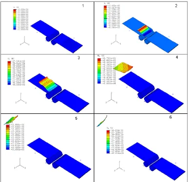
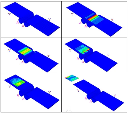
Figure 10.1.1 Response of the sample moving at 300 ft/min in the absence of viscous pressure ...65
Figure 10.1.2 Response of the sample moving at 300 ft/min in the presence of viscous pressure ...66
Figure 10.2.2 Samples moving at 300 ft/min and oriented at 300...68
Figure 10.2.3 Samples moving at 300 ft/min and oriented at 900 to conveyor length...68
Figure 10.2.4 Samples moving at 1200 ft/min and oriented along the conveyor length ...69
Figure 10.2.5 Samples moving at 1200 ft/min and oriented at 300 to conveyor length...70
Figure 10.2.6 Samples moving at 1200 ft/min and oriented at 600 to conveyor length...70
Figure 10.2.7 Samples moving at 1200 ft/min and oriented at 900 to conveyor length...71
Figure 10.2.8 Response of sample moving at 300 ft/min ...72
Figure 10.1.9 Response of the sample at 1200ft/min...72
Figure 13.1.1 10psi-MD-300 ...79
Figure 13.1.2 20psi-MD-300 ...79
Figure 13.1.3 25psi-MD-300 ...80
Figure 13.1.4 30psi-MD-300 ...80
Figure 13.1.5 10psi-MD30-300 ...81
Figure 13.1.6 20psi-MD30-300 ...81
Figure 13.1.7 25psi-MD30-300 ...82
Figure 13.1.8 30psi-MD30-300 ...82
Figure 13.1.9 10psi-MD60-300 ...83
Figure 13.1.10 20psi-MD60-300 ...83
Figure 13.1.11 25psi-MD60-300 ...84
Figure 13.1.12 30psi-MD60-300 ...84
Figure 13.1.13 10psi-CD-300 ...85
Figure 13.1.16 30psi-CD-300 ...86
Figure 13.1.17 10psi-MD-1200 ...87
Figure 13.1.18 20psi-MD-1200 ...87
Figure 13.1.19 25psi-MD-1200 ...88
Figure 13.1.20 30psi-MD-1200 ...88
Figure 13.1.21 10psi-MD30-1200 ...89
Figure 13.1.22 20psi-MD30-1200 ...89
Figure 13.1.23 25psi-MD30-1200 ...90
Figure 13.1.24 30psi-MD30-1200 ...90
Figure 13.1.25 10psi-MD60-1200 ...91
Figure 13.1.26 20psi-MD60-1200 ...91
Figure 13.1.27 25psi-MD60-1200 ...92
Figure 13.1.28 30psi-MD60-1200 ...92
Figure 13.1.29 10psi-CD-1200 ...93
Figure 13.1.30 20psi-CD-1200 ...93
Figure 13.1.31 25psi-CD-1200 ...94
Figure 13.1.32 30psi-CD-1200 ...94
Figure 13.2.1 Copypaper-10psi-MD-300 ...95
Figure 13.2.2 Copypaper-20psi-MD-300 ...96
Figure 13.2.3 Copypaper-10psi-MD30-300 ...96
Figure 13.2.4 Copypaper-10psi-MD60-300 ...97
Figure 13.2.5 Copypaper-10psi-CD-300 ...97
Figure 13.2.7 Heavy card stock-10psi-MD30-300 ...98
Figure 13.2.8 Heavy card stock-10psi-MD60-300 ...99
Figure 13.2.9 Heavy card stock-10psi-CD-300 ...99
Figure 13.2.10 Copypaper-20psi-MD-1200 ...100
Figure 13.2.11 Copypaper-10psi-MD30-1200 ...100
Figure 13.2.12 Copypaper-10psi-MD60-1200 ...101
Figure 13.2.13 Copypaper-10psi-CD-1200 ...101
Figure 13.2.14 Heavy card stock-20psi-MD-1200 ...102
Figure 13.2.15 Heavy card stock-10psi-MD30-1200 ...102
Figure 13.2.16 Heavy card stock-10psi-MD60-1200 ...103
1. PAPER RECYCLING
Recycling of paper and paper related products could be very rewarding both economically
and environmentally. It helps save landfill costs and reduces the energy requirements for
paper plants since the energy that is needed to produce recycled paper is much less than the
energy needed to produce virgin paper. Paper recycling reduces the level of usage of natural
resources. It is estimated that one ton of paper from recycled stock saves approximately 17 to
31 trees, 7000 gallons of water, 4,000 KWh of electricity, and 60 pounds of air pollutants [1].
The following chart gives an estimate of the percentage of various materials that are being
recycled [2].
Figure 1.1. Percentage of materials being recycled
Americans use 100 million tons of paper a year--for everything from daily newspapers to
books and cardboard boxes. After quick use, at least 50 million tons of paper is thrown away,
almost all of which can be recycled [3]. This means that there's about 8 billion dollars worth
Before the paper and paperboard is recycled, they need to be collected, sorted and sent to the
recycling plant. The paper recycling process typically consists of the following steps.
Collection and Transportation: Paper and paper products are collected by various recycling
centers. These centers collect the paper from households, offices and other sources. After
this, the collected material is transported to a paper recycling plant storage facility.
Sorting: Successful recycling requires clean recovered paper. Initially the paper is made free
from contaminants such as food, metal, plastic and other forms of trash. Contaminated paper
that cannot be recycled is either burned for energy or sent to land fills. After the removal of
the contaminants, the paper is sorted in order to separate it into different grades. There is no
one sorting standard used in recycling plants. The requirements of sorting changes based on
the waste paper feed they receive from various sources. But all the paper recycling plants
first needs to separate the paper into the most common grades.
Pulping and Screening: The paper moves on a conveyor to a big vat called a pulper, which
contains water and certain chemicals. The pulper chops the recovered paper into small
pieces. Heating the mixture breaks the paper down more quickly into tiny strands of cellulose
(organic plant material), called fibers. Eventually, the old paper turns into a mushy mixture,
otherwise known as pulp. The pulp is forced through screens containing holes and slots of
various shapes and sizes. The screens remove small contaminants such as bits of plastic and
De-inking: The pulp undergoes a de-inking procedure in which ink, sticky materials and
adhesives are removed.
Refining & Bleaching: During refining, the pulp is beaten to make the recycled fibers swell,
making them ideal for papermaking. If the pulp contains any large bundles of fibers, a
refining process separates them into individual fibers. If the recovered paper is colored,
color-stripping chemicals remove the dyes from the paper. If white recycled paper is being
made, the pulp may need to be bleached with hydrogen peroxide, chlorine dioxide, or oxygen
to make it whiter and brighter. If brown recycled paper is being made, such as that used for
industrial paper towels, the pulp does not need to be bleached.
Papermaking: Now the clean pulp is ready to be made into paper. The recycled fiber can be
2. SORTING OF PAPER
2. 1 Waste Paper Grades:
The most important step in the recycling procedure is the sorting of the collected paper into
different grades. Paper products with even a small amount of contaminants can alter the
quality of the final paper product. Therefore the quality of the recycled paper depends greatly
on the effectiveness of the sorting procedure. There are many ways of classifying paper into
different groups. The exact sorting requirement depends on the type of paper that the paper
recycling plant accepts. Waste paper is sorted broadly into the following categories:
1. Glossy paper
2. Office paper
3. Colored paper
4. Cardboard
5. Newsprint
6. Mixed waste
Glossy paper typically consists of magazine or coated paper. They have a heavy coating that
some paper mills do not accept, as it has to be treated separately before recycling. Office
paper is usually made from high-grade paper pulp and consists of letterheads, ledgers,
notebook, and computer papers etc. It requires less processing than other grades of paper.
Colored paper must be bleached to remove the dyes before recycling. Hence it has to be
Corrugated cardboard is made of three layers and is used for packing and shipping
containers. Boxboard is used to make cereal boxes, folding cartons, etc. These are made of
low-grade paper and are mostly recycled to make more cardboard. Newsprint (NPS) is made
of low-grade paper and cannot be mixed with office paper, as it would decrease the quality of
recycled paper. Hence it has to be sorted separately.
Even after successful sorting procedure, there are some kinds of paper products, which
cannot be recycled. Some of them which come under this category are paper with any sort of
food contamination, waxed paper, waxed cardboard milk or juice containers, oil soaked
paper, carbon paper, sanitary products or tissues, thermal fax paper, or plastic laminated
paper such as fast food wrappers, juice boxes, and pet food bags. All of these kinds of paper
come under mixed waste, which is either land filled or incinerated.
2.2 Paper Sorting Methods:
The basis for any paper sorting procedures is the identification of any mechanical, optical,
and chemical properties that vary from one set of paper samples to another set of samples and
to develop a group of sensors to identify these distinguishing characteristics. Then the sensor
output can be used to sort the paper samples into different bins using either pneumatic or
mechanical actuators.
The above methodology can be implemented in two phases. In the first phase, various
sensors that will identify a range of characteristics of the samples will be developed. In the
second phase, a network of sensors is built to exhibit a complex global behavior. In addition
to these sensors, fuzzy logic techniques can also be used for sorting [4]. Fuzzy logic
accepted only on the basis of its physical appearance. It insists on the addition of practical
experience and knowledge gained from a process rather than considering it fully controlled.
The advantage of using programmable logic during sorting is an increase in the adaptability
of the sensor network for a wide variety of feed. For example, suppose the paper mill wants
the sorting facility to sort a particular type of sample with a specific color pattern. Depending
on the requirements, one single sensor in the network might not be able to make a concrete
decision. One instance where this can happen is if the specified sample is glossy, with high
lignin content and stiff in nature. First training the sensor network using one of the specified
samples and configuring the sensor network based on the results obtained from the test
sample can solve this problem. Then the sensor network will have no problem in identifying
that particular sample from mixed paper stream.
There are only a few automated paper-sorting facilities in the US. One is at Weyerhaeuser
Corp paper recycling plant in Baltimore [5] [6] [7]. This has been recently dismantled. It
consisted of a conveyor system with conveyors of different speeds and inclinations, a sensor
module and air jet separation system. The plant can sort up to 8 tons an hour depending on
the paper being processed and the width of the sorting conveyor. At the Baltimore plant, the
paper is collected in a collection area. Paper from the collection area is fed to an inclined lift
conveyor by using a pit conveyor. The speed of the lift conveyor is more than the speed of
the pit conveyor in order to decrease the burden depth of paper. The burden depth is the
depth of paper on the conveyor. This is a crucial step in any sorting procedure because
to be correctly identified and separated. The goal is to deliver a metered, single layer stream
of paper to the sensors that come later on in the process. Heavy flow of paper from pit
conveyor begins to thin and spread out as it is fed onto the faster moving lift conveyor. Level
sensors control the burden of depth via feedback to programmable logic controllers that
determine the conveyor speed.
The paper is passed through a disc screen after the lift conveyor. The disc screen further
spreads out the paper samples and accelerates them. Another inclined conveyor is used to
transfer the samples from the disc screen to the high speed-accelerating conveyor on which
sensor stage takes place. On the high speed accelerating conveyor, the paper will be
traveling at 1,000 ft/min compared with 75 ft/min of traditional manual sorting conveyors.
To ensure that the fast moving paper does not shift on or lift from the belt, the process also
uses a comprehensive air system and a pinning device or roller.
The paper then comes under a sensor network, which the MSS Inc calls a Multi-grade sensor.
The multi-grade sensor consists of an optical sensor that detects the fluorescence levels from
Figure 2.2.1 Multi-grade sensor paper sorting setup [5]
The multi-grade sensor can classify different paper grades, including solid color sheets, ONP,
brown grades, color printed items (such as magazines and news paper inserts), off-whites,
and other coated and glossy papers. After the paper samples pass the sensor network, air jets
are used to eject paper that are classified as “to-be-ejected” into a chute. A take away
conveyor that is slightly lower than the acceleration conveyor belt picks paper objects that
are not ejected.
The most common sensors that are used during paper sorting are Lignin sensors, Gloss
Sensors, and Color sensors. The lignin sensor is used for the measurement of lignin content
in the samples. This sensor is mainly used for automated sorting of newsprint from the mixed
paper waste . Its response is sensitive to the distance between the sensor head and the sample,
glossy coatings on the surface of the paper or other shiny objects. The Color sensor is used
to identify colored samples from a mixed paper stream. The sensor setup along with the
decision-making algorithm is shown in Fig 2.2.2.
Figure 2.2.2. Sensor setup block diagram
The stiffness sensor will be useful in sorting the samples based on their relative stiffness
values. The stiffness sensor along with the remaining three sensors will be useful in
designing the decision making algorithm which exhibits the complex behavior of identifying
the samples and actuating the corresponding mechanisms to move the samples to their
respective collection bins. The air-nozzle array along with the take away conveyor system
3. STIFFNESS SENSING OF PAPER
The objective of this research was to sort the paper from mixed waste based on the
relative bending stiffness values of the paper. This kind of sorting will allow the recycling
plants to separately treat the stiff paper from the non-stiff paper during the recycling process.
This will also leads to an increase in the quality of the recycled paper and the recovery rate of
the useful paper from the mixed waste. Before developing the sensor, several stiffness
sensing techniques that are currently available were studied.
The on-machine paper stiffness sensor development has been an on-going process for over
30 years [8]. The determination of the mechanical properties is critical to the paper making
process. Almost all the paper stiffness measurement techniques are targeted for measuring
the stiffness of the paper web.
Most of the stiffness measurement techniques make use of Lamb waves to monitor the
mechanical behavior of the paper. Paper is a very complex medium. It is made of fibers
preferentially aligned in the machine direction (MD). It is a heterogeneous, viscoelastic,
anisotropic composite that is often modeled as an orthotropic plate [9-11]. Assuming that
paper can be modeled as an orthotropic material, i.e. a material that has three mutually
orthogonal symmetry planes, relationships exist between paper stiffness properties and
There are two ways of generating Lamb waves on the surface of the paper. One is a contact
method and the other is a non-contact method.
3.1 Contact Methods:
Contact transducers are used in this method for generating ultrasonic waves on the surface of
paper [12-14]. The contact transducers suffer from the fact that they are incompatible with
scanning, loading the paper, and in some cases cause damage to the sample. Problems that
plague this approach also include excessive noise due to mechanical vibrations and paper
damage where transducers contact lighter grades of paper. Monitoring of fine papers, coated
grades and paperboards is difficult. The contact method is impractical to use in a sorting
facility, as it is not possible to contact discrete paper samples on a high-speed moving
conveyor.
3.2 Non-Contact Methods:
These methods utilize either air coupled transducers or lasers to generate the Lamb waves on
the paper surface. Among the air couple transducers; piezoelectric transducers and capacitive
transducers are used mainly for stiffness testing of static paper samples. Piezoelectric
transducers have low bandwidth and low sensitivity when compared to capacitive
transducers.
The capacitive transducers are far better than air coupled piezoelectric transducers. These are
mainly limited by the poor coupling of energy between the transducer and the paper due to
An online implementation is hardly possible because the transmitter and receiver assembly
must be rotated to get the maximum transfer of energy into the paper. Also, since the sheet
must be fairly thick to excite Lamb waves (>400 µm), testing of finer grades of paper is
difficult.
Laser Ultrasonics: In this method, lasers are used to generate and detect the lamb waves
[15,16]. A short pulse of laser light is used to generate ultrasonic waves by either thermal
expansion and/or an ablation shockwave. The wave propagates along the sheet and is
detected at a precisely known distance (several millimeters) away using a non-contact
interferometric technique.
Merits of this technique include point source excitation (ideal configuration for detection of
stiffness orientation distribution), absence of measurement artifacts due to coupling medium
(insensitivity to air temperature and moisture and turbulence), and a large bandwidth.
Difficulties still exist due to sheet fluttering (also true for air-coupled transduction), and the
equipment is complex.
All of the above mentioned techniques make use of the fact that the velocity of ultrasonic
waves traveling in the paper depends on the elastic constants of the paper. Paper is assumed
to be an orthotropic material with nine elastic constants. One group of ultrasonic waves that
propagate readily in paper and are sensitive to some of the most important elastic constants
related to paper strength are Lamb waves. For a thin medium such as paper most of the lamb
The velocities Vso and Vao depend on the elastic properties of the medium and its density. The so wave contains information about tensile elasticity and the ao wave contains information about shear elasticity of the material. Lamb wave theory for an orthotropic
material predicts that the velocity of the so wave is directly related to the tensile stiffness of the sheet in the direction of wave propagation.
CT = density* V2so
CT is the tensile elastic constant
The same theory predicts that the velocity of the ao wave is directly related to the shear stiffness of the sheet in the direction of wave propagation by:
CS = density* V2ao
CS is the shear elastic constant
All the previously mentioned techniques are for testing paper webs of approximately same
thickness. These methods are aimed at calculating the exact elastic constants. These elastic
constant evaluation methods assume infinite boundary conditions in one direction, which in
the case of the paper web is the direction along the length of the web. Another assumption is
that the waves will not reflect back from that boundary. But the discrete paper samples are
much smaller than the paper web and elastic waves will be reflected from the boundaries.
This will decrease the signal to noise ratio, which implies that the phase velocity of the
waves would be harder to find. For sorting there is no need to find the elastic constants so
sorting conveyor varies widely from one sample to another. All these reasons call for a new
sensor design that is customized according to sorting facility requirements.
3.3 Bending Stiffness Sensor:
The bending stiffness sensor for the sorting facility needs to satisfy the following
requirements
1. It should be compact
2. The sensor response time should be low.
3. The sensor should be compatible with the existing conveyor systems.
The sorting process does not demand the exact stiffness values of the paper sample but rather
relative estimates of the stiffness. This eliminates the need for doing extensive computations
in real time. Considering all the above requirements, the bending stiffness sensor is built by
using a distance sensor and an air nozzle. The idea is to apply a pneumatic load on top of the
sample spanning two supports that are a known distance apart. The deflection of the sample
4. STIFFNESS SENSOR SETUP
4.1. Initial Stiffness Sensor Setup:
An infrared distance sensor was interfaced with the Motorola 68HC11 micro controller to
collect the data of the deflected paper samples due to a pneumatic load. The sensor is a
general-purpose distance-measuring sensor (GP2D12) from Sharp (corp. name etc.). The
maximum and minimum sensing range for the sensor is 100mm to 800mm. The sensor gives
an analog output in the range of 0 to 2.8 volts.
Figure 4.1.1. GP2D12 sensor calibration curve
The evaluation board for 68HC11 MCU from Technological Arts is used to interface with the
GP2D12. The micro controller has a built-in eight-channel analog to digital converter with
eight-bit resolution. The low and high reference voltages for the A/D converter are 0 volts
and 5 volts, respectively. The terminal window of the compiler was used to communicate
the end of an extended air hose. Before measuring the deflection, the sensor calibration
curves were obtained.
Figure 4.1.2. A/D converter output
It is evident from the above calibration curves that the sensor output is not linearly related to
the distance over the entire range of the sensor. But the output is close to linear within a
sensing range of 10 to 30 cm. First, in order to check that the distance sensor is not sensitive
to the target objects surface characteristics, two kinds of paper samples were used. The first
set of paper samples consisted of colored papers with a glossy surface. The second set
consisted of non-glossy color papers. The effective distance between the sensor and the
Figure 4.1.3. Sensor output for glossy paper samples
Figure 4.1.4. Sensor output for non-glossy paper samples
It is observed that the distance sensor output is sensitive to the surface characteristics of the
target. The effective distance between the sensor and the top of the two end supports was
maintained at 20 cm. The pneumatic load was applied for an average time of 0.5 sec/sample
and the nozzle inlet pressure was maintained at 25psi while being held at a distance of 25 cm
there is a flat paper on the supports. The clearance between the two supports was varied and
the corresponding digital outputs for different samples were recorded.
Figure 4.1.5. Deflection of the samples with support clearance of 6 cm
Figure 4.1.6. Deflection of the samples with support clearance of 3 cm
It was noticed that the cardboard sample does not show any deflection due to the load when
those conditions. In fact, the copy paper, with a significantly lower bending stiffness than the
other samples, could be differentiated by the digital output of the apparatus at all clearances
but the difference was greater at greater clearance. These results indicated the need for the
high-resolution distance sensor for identifying the samples with slightly varying thickness
values.
4.2. Upgraded Stiffness Sensor Setup:
The initial setup of the sensor was good enough to identify copy paper from
cardboard. In order to identify samples whose thickness values do not vary drastically, the
distance sensor needed to be upgraded. The infrared distance sensor performance is limited
by its sensitivity to the surface characteristics of the target object. Also the sensor output is
not linear over the range of the sensor. The resolution of the A/D converter of the
micro-controller was not sufficient to obtain the required data resolution. All these limitations were
overcome by making some vital changes to the sensor design.
The upgraded stiffness sensor setup is shown in Figure 4.2.1. It essentially consists of a
distance sensor, air nozzle, relay controlled solenoid valve, data acquisition system, and a
micro controller. The relay is switched by using a control signal from the micro-controller.
The analog output from the distance sensor is fed to the data acquisition board. The
Figure 4.2.1 Stiffness sensor setup
The distance sensor is a dual output, programmable ultrasonic sensor. The sensor measures
the distance of a target by sending a sound wave, above the range of hearing, at the object
and measuring the time for the sound echo to return. Knowing the speed of the sound wave,
the sensor can determine the distance of the object from the transducer element. The
measurement rate of the sensor is also programmable.
The distance sensor has a range of 15 to 427 cm. Its operation is not sensitive to ambient
light levels, the color of the target, or the target’s optical characteristics. The sensor produces
an output of 0 to 10 volts over the range of the analog window. The range of the sensor is
equal to the difference between the maximum and minimum distances that the sensor can
measure. These limits can be set to be equal to any value within 15cm to 427cm. This feature
can be used to increase the resolution of the sensor to any required value. The calibration
curves for the distance sensor with different operating ranges are shown in figure 4.2.2 and
Figure 4.2.2. Distance sensor output when the range is equal to 40 cm
Figure 4.2.3. Distance sensor output when the range is equal to 6 cm
One more parameter that influences the measurements is the response time of the distance
This affects the measurement rate of the sensor, which is the repetitive rate at which the
sensor measures distance. The sensor’s calculated distance can be set to change at a slow or
fast rate. This will affect how quickly the sensor output will change. With a fast rate of
change the outputs respond with the farthest of every two-distance measurements. The fastest
5. STATIC BENDING STIFFNESS SENSOR
5.1. Static Testing Of Paper Samples:
In order to evaluate the performance of the distance sensor, four paper samples that are
commonly found in the input feed to the recycling plant were tested statically. The paper
samples were made to sit on two end supports with a gap separating the supports and the
pneumatic load was applied on top of the samples by using the air nozzle.
Before the samples were tested, the load profile of the nozzle was obtained by measuring the
force exerted by the air jet when the nozzle is held at a specified height above the top surface
of the sample. An electronic balance with a flat weighing surface was used for measuring the
load. A rigid plate with a small hole in the center was attached to the top of the balance. A
clearance of about 3mm was maintained between the plate and the top face of the weighing
balance. The spatial force map was obtained by moving the balance along with the rigid plate
on a planar grid in the x-y plane. The distance between the nozzle and the top surface of the
balance and the nozzle inlet pressure were set to be equal to 25.4 cm and 20 psi respectively.
The paper sample properties were measured according to TAPPI standard procedures. For
the static stiffness measurement, the sensor response time was programmed to be equal to 25
msec. The response time is not a critical factor for static testing of samples because the
Figure 5.1.1. Spatial load distribution of the nozzle
Table 5.1.1. Mechanical properties of paper samples
Paper grade Note Book Filler Paper
Medium
card
stock
Heavy
card
Stock
Specialty
card
stock
Thickness (µm) 105 206 229 234
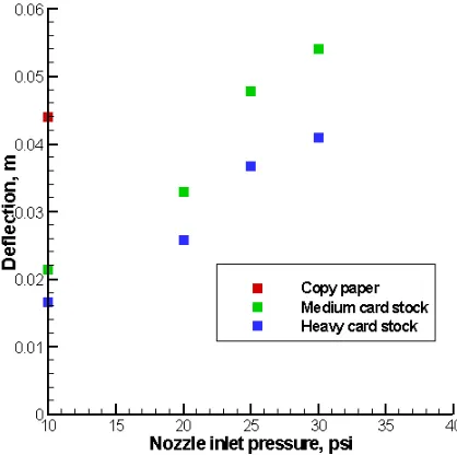
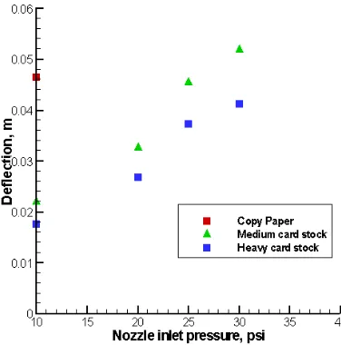
There are two ways of loading the sample. The sample can either be placed over the
conveyor supports in such a manner that its machine direction is along the length of the
conveyor or it can placed such that its cross machine direction is along the conveyor length.
But for both the configurations, the samples are loaded vertically. The response of the
samples under the above mentioned loading conditions is shown in the following figures.
Figure 5.1.3. Deflection Vs Basis weight
The deflection of the paper due to a vertical load on its top surface is greatly influenced by
the thickness and basis weight of the paper sample. The static testing of the samples gives an
idea about the behavioral pattern of the deflection values that might occur during the actual
dynamic loading process. But the deflection values from the static deflection tests cannot be
used for creating the lookup table for the sorting algorithm because the loading and boundary
conditions in a dynamic loading procedure are different from the static boundary and loading
conditions. The spread of the nozzle that was used for static testing of the sample is wide.
This will affect the repeatability of the experiments and it also leads to wastage of the
The nozzle used for the static testing of the samples produced a cone shaped loading profile.
This complex loading profile is also difficult to simulate in the analysis model. To avoid
these undesirable effects, several nozzles with different profiles were investigated in order to
find a more effective nozzle for the sorting procedure. Among these, a flat fan nozzle, and a
cylindrical pattern nozzle were found to be useful. The flat fan nozzle produces a spray
pattern that has a fan configuration in one axis (a line). The cylindrical stream nozzle
produces a concentrated direct stream of air from the nozzle.
Figure 5.1.4. Nozzles used for applying the load on the paper sample
The total load exerted by both the cylindrical nozzle and the flat fan nozzle was found for
various pressures by following the same procedure that was used for finding the spatial load
distribution of the conical spread nozzle. Since the spread area of both the flat fan and
cylindrical nozzles is small compared to the conical spread nozzle, the balance was not used
Figure 5.1.5. Cylindrical nozzle load profile
The total load exerted by the air exiting from the cylindrical nozzle at a particular value of
inlet pressure remains almost constant up to a distance of 7 inches from the nozzle head. The
total load exerted by the flat fan nozzle drops off drastically as the distance between the
nozzle outlet and the paper surface increases.
The spread of the cylindrical nozzle at different pressures was found by using two filter
papers; one of them was made wet by using a colored dye while the other one was kept dry.
The nozzle was made to operate continuously and the dry filter paper was placed on a flat
surface perpendicular to the nozzle orientation. The wet filter paper was placed on top of the
dry paper and removed after a few seconds. On the area where the intensity of the load was
high, the wet paper left a color impression on the surface of the dry paper.
The geometric shape of the exposed surface is almost circular. So, the mean diameter of the
circular spread is found by running the same test several times. The load intensity for the
cylindrical nozzle is found by dividing the total load by the spread area. The test results are
Table 5.1.2. Circular spread area for cylindrical nozzle
SPREAD AREA, sq.mm
Nozzle Height 1" 2"
5 psi 77.42 166.86
75.06 144.42
75.46 169.19
Mean 75.99 160.16
Standard Deviation 1.26 13.68
Standard Error 0.73 7.89
Nozzle Height 1" 2"
10 psi 73.90 180
73.52 124.59
65.64 153.20
Mean 71.02 152.59
Standard Deviation 4.67 27.71
Standard Error 2.69 15.99
Nozzle Height 1" 2"
20 psi 72.75 154.32
65.64 143.34
68.59 146.59
Mean 68.99 148.08
Standard Deviation 3.57 5.64
Standard Error 2.06 3.26
Nozzle Height 1" 2"
25 psi 51.21 141.73
54.15 149.33
53.49 146.59
Mean 52.95 145.88
Standard Deviation 1.55 3.85
Standard Error 0.89 2.22
Nozzle Height 1" 2"
30 psi 51.21 142.26
50.25 145.50
53.17 143.34
Mean 51.54 143.70
Standard Deviation 1.48 1.65
6.PILOT PLANT TRIALS
In order to identify the problems that might arise during the working of the sensor on a
high-speed moving conveyor, the stiffness sensor was tested at MSS Inc, Nashville, TN. The
dynamic testing of the sensor also helps in identifying the variables that will influence the
deflection of the samples when the sample is loaded dynamically.
The conveyor used for testing the sensor has a variable frequency drive that can be used to
change the speed of the conveyor. The conveyor is 12” wide and 48” long. The conveyor belt
is made of Poly vinyl chloride and is considered a smooth surface. Two similar conveyors are
placed one after another with a gap of 1.58 inches. The diameter of the head roller of the
conveyor is 4 inches. The ultrasonic distance sensor was installed in the gap between the two
conveyors at a distance of 7” below the conveyor top surface. The analog output window of
the sensor was adjusted such that it produced a maximum output voltage of 10 volts at a
distance of 7 inches from the sensor head. This distance is also equal to the sensor head
distance from the top surface of the conveyor. The minimum limit of the analog output
window starts at a distance of 4.5 inches from the sensor head. Therefore the output of the
sensor varies from 0 to 10 volts with in a span of 2.5 inches.
The nozzle was placed perpendicularly at a distance of 1 inch above the top of the
conveyor surface. The nozzle and the distance sensor have the same vertical axis of
used to switch the nozzle on and off. Since the nozzle is going to be operated at low
pressures, it is not going to affect the performance of the ultrasonic distance sensor.
Figure 6.1. Paper sample sitting on two conveyors
Table 6.1 Samples tested on the moving conveyor
No. Name Thickness (µm) Grammage (g/m2)
1 Copy Paper 103.8 77.27
2 Yellow Ruled Paper 106.5 75
3 Filter Paper 110.5 78.43
4 Medium Card Stock 206 145
5 Heavy Card Stock 229 200
6 Specialty Card Stock 234 175
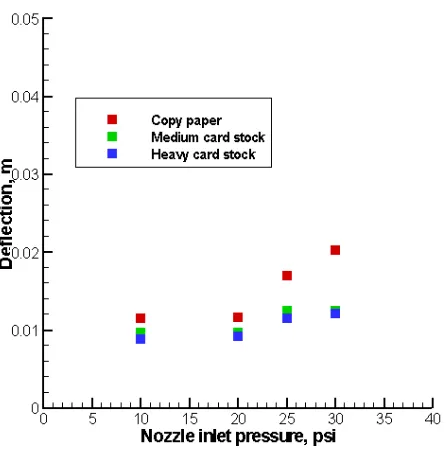
Figure 6.2 Deflection of the samples when nozzle inlet pressure is equal to 5psi and nozzle clearance above the sample is equal to 1 inch
Figure 6.4 Dynamic loading of the paper sample
The results indicate that the sensor output is sensitive to the stiffness of the samples. For the
same nozzle inlet pressure, the deflections of the paper samples are higher for the case in
which the sample is held at 1 inch above the conveyor surface. Therefore the sensor
resolution will be better if the nozzle is held close to the conveyor surface. In order to
increase the sensitivity of the sensor for the case in which the nozzle is held at a greater
distance from the conveyor surface, the nozzle inlet pressure needs to be increased to
compensate for the pressure loss due to an increased spread area.
During some of the tests, thin samples such as copy paper and yellow ruled paper failed to
jump the gap between the conveyors. Moderately thick samples such as Medium stock
paper, Heavy stock paper, and Specialty stock paper did not have a problem in clearing the
behavior of the thin samples. By increasing the speed, the inertial effects associated with the
7. STIFFNESS SENSOR CHARACTERIZATION
7.1. Variables Influencing The Paper Deflection:
Before creating a methodology for identifying the samples based on their relative stiffness
values, the different variables that will influence the deflection of the paper need to be
known. The most influential variables are given below:
1. Thickness of the sample: This is the most influencing variable in determining the
flexural rigidity of the paper sample. Samples with higher values of thickness have
larger values of flexural rigidity.
2. Orientation of the sample relative to the conveyor belt: The sample may be
positioned over the conveyor supports in such a manner that its machine direction is
along the length of the conveyor or else it can oriented such that its cross machine
direction is along the conveyor length. Generally, for machine made paper the
Young’s modulus in the machine direction is twice the Young’s modulus in the
cross-machine direction. Therefore, the samples traveling in the cross-machine direction deflect
less than the samples traveling in cross-machine direction.
3. Basis weight: Basis weight of the paper is directly proportional to its thickness.
Therefore with higher basis weight, the deflection will be lower. The basis weight of
the sample is also related to the density of the sample. With a higher sample density,
the kinetic energy will also be higher influences the deflection of the paper in motion.
4. Distance between the conveyors (gap): This indicates the distance that the sample has
to cross while the load is applied on top of it. With a larger gap, the sample deflection
will be larger. But increasing the gap will cause some of the low stiff samples to fall
5. Intensity of the loading: For higher load intensity, the sample deflection will also be
higher. The load profile needs to be fine in order to lower the error in
decision-making.
6. Conveyor speed: For a higher conveyor speed, the sample will have a lower
deflection. This is a result of the high inertia of the moving sample.
7. Coefficient of friction between the conveyor and the paper surface: For a higher
coefficient of friction, the sample deflection will be lower because the friction resists
the sliding of the paper over the roller surface when the load is applied.
7.2 Sensor Characterization:
The dependence of the deflection of the paper sample on the above-mentioned variables
makes it complicated to build an analytical model to predict the sample deflection at various
conveyor speeds and the nozzle loads. Therefore the following approach is identified as the
suitable one for building the decision-making algorithm.
Step1: Among the recovered paper grades, some of the most frequent grades are identified.
The selected paper grades are tested mechanically to find the material constants.
Step2: A finite element analysis model of the system is built. The original loading and
boundary conditions on the sample are simulated in the FEA model. The deflection values
from the finite element simulation are used in building the look-up tables that can be used by
8. PAPER MATERIAL MODEL
8.1 Paper Material Properties:
The mechanical properties of the paper samples are needed for building the material
model for the finite element analysis. The accuracy of the material model influences the
accuracy of the simulation outputs. Therefore it is important to find the accurate material
model to represent the paper during the analysis.
The material model defines the constitutive relationship between the stress and strain in a
given material. Even though paper is highly anisotropic at the microscopic level, it is
considered as a homogenous orthotropic material at the macroscopic level. The
constitutive relationship for an orthotropic material is
− − − − − − = 23 13 12 33 22 11 23 13 12 3 2 23 1 13 3 32 2 1 12 3 31 2 21 1 23 13 12 33 22 11 / 1 0 0 0 0 0 0 / 1 0 0 0 0 0 0 / 1 0 0 0 0 0 0 / 1 / / 0 0 0 / / 1 / 0 0 0 / / / 1 σ σ σ σ σ σ ν ν ν ν ν ν γ γ γ ε ε ε G G G E E E E E E E E E
Where νijis the Poisson’s ratio that characterizes the transverse strain in the j direction,
when the material is stressed in the i direction. For orthotropic materials vij and νji are
related by j i j i j
i /E ν /E
The material constants also need to satisfy the material stability requirements, which are given below
(
)
(
)
(
)
0 2 1 / / / 0 , , , , , 13 32 21 13 31 32 23 21 12 3 2 23 3 1 13 2 1 12 23 13 12 3 2 1 f p p p f v v v v v v v v v E E E E E E G G G E E E − − − − ν ν νSince the paper is very thin, plane stress shell elements are used to model the paper sample.
Under plane stress conditions, only values of E1, E2,v12,G12 andG23 are required to define the orthotropic paper material. In each of the plane stress elements the out of plane stress
isσ33 = 0. The shear moduli G13 and G23 are included to model the transverse shear deformation.
The material stability criterion for the plane stress elements requires the material constants to
satisfy the following conditions
(
1 2)
12 23 13 12 2 1 / 0 , , , , E E v G G G E E p f
For machine made paper, the three principal material directions are along the machine
direction, cross machine direction and the thickness direction. The Young’s modulus in
machine and cross machine direction can be obtained by tensile testing the paper samples in
12
G can be accurately obtained with only a few data points for E versus the orientation angle
plus one good value for in plane Poisson’s ratio v12. The goal of this method is to perform the measurements of the Young’s moduli in the optimum angular region (the so-called error
boundary) to achieve the best accuracy in the determination ofG12. A least square algorithm is used to estimate the shear modulus that is best fitted to the experimental data.
The basic equation that describes the elastic constants in two-dimensional orthotropic case is
(
cos /) (
sin /)
cos sin(
(
1/) (
2 /)
)
.(8.1.1)/
1 E 4 E 4 E 2 2 G v E Eq
md xy xy
cd
md + + − LL
= θ θ θ θ
θ
Where
=Young’s modulus measured in uniaxial tension test of off axis strip (angle θ from the
machine direction).
md
E = Young’s modulus measured in uniaxial tension test of machine directional strip
cd
E = Young’s modulus measured in uniaxial tension test of cross directional strip
xy
G = In plane shear modulus
xy
v = In plane Poisson’s ratio
From Eq. (1)
(
)
.(8.1.2)sin cos 2 sin cos 1 sin cos 2 2 4 4 2 2 Eq E v E E E G md xy cd md
xy LLL
The objective of the optimization method is to choose a procedure such that the coefficients
of variation of the experimental values of Emd,Ecd,Eθ,and vxy do not have too much effect
on the coefficient of variation of the estimated shear modulus.
If the value of cos2θsin2θ which is associated with Poisson’s ratio in Eqs.8.1.1 and 8.1.2
approaches zero, the effects of the COV of the Poisson ratio on the COV of estimated shear
modulus would decrease. To see the influence of the experimental error of Eθon the
estimation of shear modulus Eθis perturbed from its true value and remaining material
constants are kept unperturbed, as θ changes from 0° to90 . The shear modulus estimated 0
in this way was compared with the true shear modulus and the differences were plotted as
percentages. The minimum error boundary region is found from the error plot. The angle of
minimum error boundary is dependent upon the elastic constants of the material. Poisson
ratio does not affect this angle. The anisotropy of shear moduli, which describes the variation
of in-plane shear moduli with orientation in the sheet, does affect the location of the point.
However, for paper materials, the anisotropy of the shear moduli is restricted to values from
0.992 to 1.169 experimentally. Due to this, the location of the minimum error boundary was
affected by less than 1 which is quite inconsequential. Thus for paper materials it can be 0
safely said that the anisotropy of shear moduli does not affect the location of the point of
minimum error boundary significantly.
The anisotropy of Young’s moduli, which is defined as the ratio of Emdto Ecd has some
boundary curve that is a function of anisotropy of the Young’s moduli was used to test
off-axis samples that are cut at an angle of θ −5,θ,θ +5; where θ is the angle of minimum
error boundary.
8.2 Paper Testing:
A bench-top miniature tensile tester was used to test paper samples. The tester is equipped
with a high resolution LVDT and a load cell. The sample is loaded between two supports on
the test frame. The speed of the movable head of the tester is controlled by a control signal
from the micro-controller to the stepper motor.
Figure 8.2.2. Miniature material tester
Three grades of paper that are commonly found in the recovered paper to the recycling plant
were tested for material properties using the tensile tester. Thin strips of paper of uniform
width were cut both in machine direction and cross machine direction and tested to get the
Young’s modulus in machine direction and cross-machine direction. Then the anisotropy of
the Young’s moduli was found by finding the ratio of EmdtoEcd. Based on the anisotropy of
the Young’s moduli the angle of minimum error boundary was found from the error
boundary curve that was depicted by Seo, Y.B et al [17]. The results of the tensile tests on
Figure 8.2.3. Copy paper stress strain curves in different directions to the machine direction
Figure 8.2.5. Heavy card stock stress strain curves in different directions to the machine direction
The following least square algorithm was used to find the in plane shear modulus of the
paper samples. Let 2 , , 3 , 2 , 1 1 sin sin cos 2 cos 2 sin cos 1 4 2 2 4 2 2 − = − + − = = n i E E E v E i X i X i cd i md i i xy md i i i K θ θ θ θ θ θ θ Where
n = number of Young’s moduli used for optimizing
xy
G
The Euclidean norm is defined by the expression:
∑
+= ( 1 2 )
) 2 , 1
(X i X i SX i X i
F
is minimized for n determinations of Young moduli in order to optimize S.
The partial differentiation of the above expression with respect to S is:
( )
( )
∑
∑
∑
∑
∑
− = ⇒ = + = + 2 2 1 2 1 0 2 1 2 1 2 0 ) 2 1 ( 1 2 i i i i i i i i i X X X S X X X S X SX Xand the calculated in-plane shear modulus Gxy is:
( )
∑
∑
− = = i i i X X X S Gxy 2 1 1 1 2The Young’s modulus values obtained from the material testing of paper are used in
determining the in-plane shear modulus. The Poisson’s ratio was taken to be equal to 0.15.
The Young’s moduli in the machine direction, cross-machine direction and off-axis direction
values are calculated by using the slope of the best-fit line in the linear region of the
Table 8.2.1 Elastic constants for copy paper
Table 8.2.2. Elastic constants for Medium card stock
8.3 Paper Plasticity Model:
Most of the plasticity models, which define the relationship between the stress and strain
when the material starts deforming plastically, are “incremental” theories [18]. In these the
mechanical strain is decomposed into an elastic part and plastic part. In these models, the
true strain values are used instead of nominal strain values. This is helpful when the strains
are very large such as in a ductile material. True strain,ε also called logarithmic or natural
strain, is defined such that every incremental length change is divided by the current length.
o l l l l l dl l dl d o ln / = = =
∫
ε ε εThe true strains for equivalent deformation in tension and compression are identical except in
sign. The advantage of true strains over the nominal strains is that the true strains are
additive, the total strain being equal to sum of the incremental strains. When the strains are
small, then true and engineering strains are nearly equal.
Plasticity models have a yield surface, a flow rule and the evolution laws that define the
hardening criteria. Yield criteria is a mathematical expression whose primary use is to predict
if or when yielding will occur under combined stress states in terms of particular properties
of the material being stressed.
The most general form is
C f(σx,σy,σz,τxy,τyz,τzx) =
In terms of Principal stresses, the yield criterion can be expressed as
C f(σ1,σ2,σ3) =
The flow rule defines the inelastic deformation that occurs if the material point is no longer
responding purely elastically and the evolution laws govern the way in which yield and flow
definitions change as inelastic deformation occurs. Since the paper is orthotropic in nature,
Hill’s yield criterion that is used for anisotropic materials is used for defining the plasticity
model. Hill’s stress function is an extension of the Mises function to model anisotropic
behavior.
The function is
2 2
2 2
2
2 ( ) ( ) 2 2 2
) (
)
( F y z G z x H x y L yz M zx N xy
f σ = σ −σ + σ −σ + σ −σ + τ + τ + τ
in terms of rectangular Cartesian stress components, where F, G, H, L, M, N are constants
obtained by tests of material in different orientations. These constants are defined as
Where σois the reference yield stress and X, Y, Z are the tensile yield stresses and R, S, T are
the yield stresses in shear. Plastic material behavior is predicted using an isotropic hardening
formulation. The following is the flow rule that governs the hardening:
λ σ
ε f d
d j i pl j i ∂ ∂ =
Where εplijis the plastic strain; dλ is a scalar multiplier that depends on the slope of the
hardening curve; j i f σ ∂ ∂
is the normal to Hill’s yield surface. The yield stresses in machine
and cross-machine directions are determined directly from the stress-strain curves. For all
properties that could not be obtained from the tests conducted, engineering estimates were
made. These were based on the material properties obtained by Baum and Habeger [19] for
milk carton stock. The heavy card stock and medium card stock have properties similar to the
milk carton stock.
The Orthotropic elastic and anisotropic plasticity material model is supported only in
ABAQUS/Standard analysis code but not in ABAQUS/Explicit. ABAQUS/Standard uses
Hilber-Hughes-Taylor operator for integration of the equations of motion. This offers the use
of all elements in ABAQUS but can be slower than Explicit. ABAQUS/Explicit uses the
central difference operator and is more robust when handling complex contact problems. But
Explicit has fewer element types than ABAQUS/Standard. However, the method provided in
ABAQUS/Explicit has some important advantages. In explicit problems the analysis cost
rises only linearly with the problem size, whereas the cost of solving the nonlinear equations
Therefore ABAQUS/Explicit is suitable for simulating the Paper-Conveyor dynamic
problem.
Table 8.3.1. Yield stresses for different paper grades
Yield Stress (Copy Paper)
Value Anisotropic Yield Stress Ratios
Method
X 25.55 MPa 1 Measured
Y 12.8335 MPa 0.503 Measured
Z 13 MPa 0.509 Estimated
R 13 MPa 0.881 Estimated
S 1 MPa 0.068 Estimated
T 1 MPa 0.068 Estimated
σo 25.55 MPa Estimated
Yield Stress
(Medium card stock)
Value Anisotropic Yield Stress Ratios
Method
X 15.20 MPa 1 Measured
Y 14.22 MPa 0.936 Measured
Z 13 MPa 0.855 Estimated
R 13 MPa 1.481 Estimated
S 1 MPa 0.114 Estimated
T 1 MPa 0.114 Estimated
σo 15.20 MPa Estimated
Yield Stress
(Heavy card stock) Value Anisotropic Yield Stress Ratios Method
X 12.79MPa 1 Measured
Y 11.23 MPa 0.878 Measured
Z 13.00 MPa 1.016 Estimated
R 13.00 MPa 1.759 Estimated
S 1.00 MPa 0.135 Estimated
T 1.00 MPa 0.135 Estimated
9. FINITE ELEMENT MODEL
In order to find the deflections of the selected paper grades when they are moving on
high-speed conveyor, a finite element analysis model was built. Initially the model was built in
ABAQUS/Standard environment. Because of significant nonlinearity involved in the model,
the ABAQUS/Standard code was unable to converge. So, the model was built in
ABAQUS/Explicit environment, which is suitable for transient dynamic analysis problems.
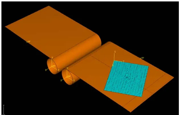
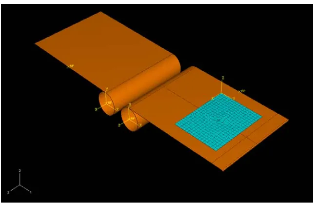
9.1 Model Geometry:
Conveyor surface is modeled as an analytical rigid surface and the paper is modeled as
orthotropic lamina. The material constants, which were found using the tensile tester and the
error minimization algorithm, are used for building the material model.
Since the lateral (in-plane) dimensions of the paper are much larger than the thickness of the
paper, plane stress shell elements are used for modeling the paper surface. These elements
also allow transverse shear deformation. Kirchoff’s thin shell theory is used for the 3D
model, implying that a material line that is originally normal to the mid-surface of the shell
elements remains so throughout the deformation. Transverse shear stress acts as penalty
function to impose Kirchoff’s constraints.
The shell elements that are used for modeling the paper also account for finite membrane
strains and arbitrarily large rotations. Each shell element has four nodes at which element
variables are calculated. These elements have nodes only at the corners and use linear
interpolation in each direction to find the displacements at any other point in the element.
Each node has six degrees of freedom these include both the rotational and translational
degrees of freedom. Even though the shell elements allow transverse shear deformation, it
becomes very small as the shell thickness decreases. The in-plane dimensions of the paper
sample are specified to be equal to 11”x8.5”.
The machine direction of the paper is specified to be parallel to the length of the paper and
cross-machine direction is specified to be parallel to the width of the paper. The machine and
cross machine directions of the paper corresponds to the in-plane principal material
directions of the paper. The rollers at the end of the conveyor surface are modeled separately
surface. This will also allow separate boundary conditions for the rollers. Explicit dynamic
analysis procedure is used to solve the nonlinear equations of motion.
9.2 Contact Interactions:
Contact interactions are used to model the contact between different surfaces in the model.
Contact modeling involves two steps. In the first step various surfaces that might come into
contact during the analysis procedure are identified. Then these surfaces are coupled together
by specifying them as contact pairs. In the second step mechanical property models are
assigned to the contact pairs. The contact property model specifies the normal and tangential
behavior of the surfaces when they come into contact.
The normal behavior between the paper surface and the conveyor surface is specified as hard.
The “Hard” contact relationship minimizes the penetration of the shell element nodes into the
conveyor surface and does not allow transfer of tensile stress across the interface. When the
surfaces are in contact, any contact pressure can be transmitted between them. The surfaces
separate if the contact pressure reduces to zero. Separated surfaces come into contact when
the clearance between them reduces to zero.
When the surfaces are in contact they usually transmit shear as well as normal forces across
their interface. The relationship between these two force components is expressed in terms of
stresses at the interface of the bodies. This relationship is known as the friction between the
contacting bodies. Classical isotropic Coulomb friction model is used to specify the
![Figure 2.2.1 Multi-grade sensor paper sorting setup [5]](https://thumb-us.123doks.com/thumbv2/123dok_us/1348755.1167751/21.612.128.502.71.304/figure-multi-grade-sensor-paper-sorting-setup.webp)